Article

A Dynamic Remote Sensing Data-Driven Approach for Oil Spill Simulation in the Sea

1
Institute of Remote Sensing and Digital Earth, Chinese Academy of Sciences, Beijing 100094, China
2
University of Chinese Academy of Sciences, Beijing 100049, China
3
School of Computer Science, China University of Geoscience, Wuhan 430074, China
4
Space Science and Engineering Center, University of Wisconsin-Madison, Madison, WI 53706, USA
*
Author to whom correspondence should be addressed.
Remote Sens. 2015, 7(6), 7105-7125; https://doi.org/10.3390/rs70607105
Submission received: 20 January 2015 / Revised: 10 May 2015 / Accepted: 15 May 2015 / Published: 29 May 2015

Abstract

:
In view of the fact that oil spill remote sensing could only generate the oil slick information at a specific time and that traditional oil spill simulation models were not designed to deal with dynamic conditions, a dynamic data-driven application system (DDDAS) was introduced. The DDDAS entails both the ability to incorporate additional data into an executing application and, in reverse, the ability of applications to dynamically steer the measurement process. Based on the DDDAS, combing a remote sensor system that detects oil spills with a numerical simulation, an integrated data processing, analysis, forecasting and emergency response system was established. Once an oil spill accident occurs, the DDDAS-based oil spill model receives information about the oil slick extracted from the dynamic remote sensor data in the simulation. Through comparison, information fusion and feedback updates, continuous and more precise oil spill simulation results can be obtained. Then, the simulation results can provide help for disaster control and clean-up. The Penglai, Xingang and Suizhong oil spill results showed our simulation model could increase the prediction accuracy and reduce the error caused by empirical parameters in existing simulation systems. Therefore, the DDDAS-based detection and simulation system can effectively improve oil spill simulation and diffusion forecasting, as well as provide decision-making information and technical support for emergency responses to oil spills.

Graphical Abstract

1. Introduction

In recent years, frequent oil spills have affected the environment, economy and quality of life for coastal inhabitants [1]. For example, the Deepwater Horizon oil spill, which occurred on 20 April 2010, killed 11 people and presented an unprecedented threat to Gulf of Mexico marine resources [2]; the Dalian Xingang oil spill incident, which happened on 16 July 2010, spread an estimated 1500 metric tons of crude oil into the Yellow Sea and stretched over 430 km2 of ocean, with 12 km2 severely affected [3]; on 4 and 17 June 2011, two separate oil spill accidents occurred at platforms B and C of the Bohai Penglai 19-3 oilfield, and they caused 5500 km2 of seawater pollution, roughly equivalent to 7% of the Bohai Sea area; and in the same year, on 12 July, the Liaoning Suizhong oil spill incident spread an estimated 0.1 to 0.15 cubic meters of crude oil into the Bohai Sea and stretched over 1 km2 of ocean, according to the China State Oceanic Administration (SOA) [4].
Remote sensing technology plays an important role in monitoring marine pollution caused by oil spills. There are numerous broad uses of oil spill remote sensing [5,6], such as mapping of spills [7,8], surveillance and general slick detection [911], direction of oil spill countermeasures [12] and determination of slick trajectories [13]. Due to the long revisit time for satellites, it is difficult to have oil slick time series for long periods after the first observation. Therefore, many scholars have combined remote sensing detection with numerical models, so as to provide continuous tracking of the oil range and spill diffusion direction. For example, for the first time, the combination of satellite images of surface oil slicks with Lagrangian trajectory models has been implemented in the operational oil spill trajectory hindcast/forecast for the Deepwater Horizon oil spill [2,14,15]; Zodiatis et al. (2012) used the MEDSLIKoil spill model to forecast the drift and spreading of oil slicks detected from satellite images using MyOcean ( www.myocean.eu.org) forecasting data, through the implementation of MEDESS-4MS( www.medess4ms.eu) project services [16]; and Dominicis et al. (2013) used the MEDSLIK-II Lagrangian marine model to simulate oil slick transport and transformation processes for realistic oceanic cases and the model initialized using the slick position and slick shape provided by satellite systems, both SAR (synthetic aperture radar) and optical images [17].
However, the growth and evolution mechanisms of oil particles are very complicated, and the fate of the oil spilled into the ocean depends on many factors, including transport and dispersion by ocean circulation along with chemical transformations and biological consumption of the oil itself. A system for tracking the oil, both at the surface and at depth, was nonlinear, time-varying and multivariable, and it was difficult to analyze and forecast the complex movement of oil particles in an exact way [18]. As for the combined model, the location and size of the surface oil slick are inferred from satellite images, and they should be frequently re-initialized to reduce the forecast errors, which could be accumulated from the initial locations (conditions), as learned from the rapid response to the Deepwater Horizon oil spill in the Gulf of Mexico [2,14,15]. However, other related model parameters, such as data on wind forcing, sea surface temperature and sea currents, are from empirical values, model calculations or some meteorological data centers [17], and they may not be precise. Then, the inaccurate data could affect the model’s predictive accuracy. Therefore, we should explore some new methods to minimize the influence of accumulated errors.
DDDAS is a new paradigm for application simulations and measurements. It entails both the ability to incorporate additional data into an executing application and, in reverse, the ability of applications to dynamically steer the measurement process. Through the synergistic feedback and control loop between application simulations and measurements, the paradigm offers the promise of improving modeling methods and augmenting the analysis and prediction capabilities of application simulations and the effectiveness of measurement systems [19]. We introduced the DDDAS into oil spill remote sensing detection and numerical simulation in order to minimize the influence caused by inaccurate parameters and to improve the predictive accuracy of oil spill simulations. In order to test our DDDAS-based oil spill simulation approach, we chose the Penglai 19-3B platform, Dalian Xingang and Liaoning Suizhong oil spill accidents as experimental cases. For conveniently describing the introduced methodology completely, we chose the Penglai 19-3B platform oil spill incident as the key experimental case, and the other two cases were selected as method validation cases.

2. Oil Spill Remote Sensing Detection Techniques

2.1. Oil Spill Remote Sensing

Remote sensor data can provide information about the oil spill area, type and thickness in a large area, so as to guide maritime surveillance vessels and aircraft to enforce monitoring [20]. Among satellite sensors, active microwave sensors, like synthetic aperture radar (SAR), which has relatively wide coverage and day/night/all-weather imaging capabilities, have been widely used to provide valuable synoptic information about the position and size of oil spills and seeps [2123]. Envisat (Environmental Satellite), launched on 1 March 2002, is an Earth-observing satellite still in orbit. Envisat Advanced Synthetic Aperture Radar (ASAR) operates in the C band in a wide variety of modes. The wavelength is 5.6 cm, and it has many unique properties, such as multipolarity, variable viewing angles and wide imaging. The wide swath (WS) mode, the only one specifically designed for detecting offshore oil spills by international radar satellites, provides better coverage range and radiation accuracy [24,25].
Due to the slick’s damping of small-scale capillary waves and short gravity waves, areas covered by oil appear as dark features if the wind speed, wave height, SAR observation incidence angle and radar beam are suitable [26]. In addition, as the oil spill depth decreases, the gray values increase slightly [27]. Thus, we can use the gray difference between the oil spill and the seawater to extract the contour and area of oil slicks with threshold methods [28].

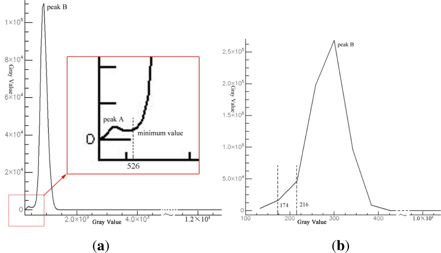
2.2. Oil Spill Detection

The Penglai 19-3 oil field is located in the south central Bohai Sea 11/05 contract area and the Tan-Lu fault zone, which lies in the northeast end of the Bonan uplift [29]. The exploitation range is 120°01 E to 120°01 E, 38°17 N to 38°27 N. The Bohai Sea is semi-closed, with an average water depth of 18 m [30] (Figure 1). The 2011 oil spills were the first large-scale subsea oil spills in Mainland China in recent years. According to ConocoPhillips China statistics, these accidents resulted in the release of approximately 700 barrels of oil and 2500 barrels of mineral oil-based drilling mud onto the seabed [33].
In this study, we chose three ASAR WS mode images as the Bohai Penglai 19-3 monitoring data of the oil spill picked up by remote sensors, obtained on 11, 14 and 22 June 2011. After the geometric precision correction and an enhanced Lee filter were applied[31,32], a subset of the image area (800 × 800) was extracted at the Penglai 19-3B and C oil platforms (Figure 2).
As Figure 2 shows, numerous oil slicks were observed northeast of the 19-3B platform on 11 June (Figure 2a), and they drifted southeast on 14 June (Figure 2b); however, the integrated oil slicks disappeared by 22 June (Figure 2c). The floating oil was cleaned up by 22 June, which is consistent with the China State Oceanic Administration’s 2011 Bohai Bay Oil Spill Accident Investigation Report by the Joint Investigation Team.
Given the grayscale and specific outlines of the oil slick, the single threshold method was used to extract information about the oil spill from the ASAR images [34,35]. Since there are generally two peaks in the histograms of ASAR images that contain oil spill information, we chose the minimum between the two peaks as the threshold values to distinguish the oil slicks from the background sea area. Because the oil was cleaned up by 22 June, we chose the 11 and 14 June ASAR images from which to extract information about the oil. By using the ENVI band statistical tools, the two image histograms can be drawn (Figure 3).
As Figure 3a shows, there were two significant peaks, A and B, and we selected the minimum gray value 526 between the two peaks as the segmentation threshold to extract information about the oil spill. However, for the 14 June ASAR image histogram (Figure 3b), the smaller gray peak is not obvious, because the oil spill area was small compared with the entire image. There was only one peak in the 14 June ASAR image histogram. We cannot use the minimum gray value between the two peaks to determine the segmentation threshold. Nevertheless, due to the oil slick’s “dark” features in the SAR images, the 14 June ASAR image histogram shows two distinct turning points at the 174 and 216 gray levels. We chose 174 and 216 as alternative segmentation thresholds. Through many experiments and comparisons, 216 is the segmentation threshold of the 14 June image for extracting information about the oil spill.
After the single threshold segmentation, the results for the 11 and 14 June ASAR images are as shown in Figure 4.
To verify the results, oil slick samples were selected from the original ASAR images. The overall classification accuracy was 92.1726%, and the kappa coefficient was 0.9425. As we know, the overall classification accuracy is calculated by summing the number of pixels classified correctly and dividing by the total number of pixels. The kappa coefficient (K) is a discrete multivariate technique used in accuracy assessment. K > 0.80 represents strong agreement and good accuracy; 0.40 < K < 0.80 is in the middle, and K < 0.40 is poor. The extraction results could serve as evaluation standards of oil spill forecast models [36].

3. Oil Spill Simulation Techniques

3.1. Oil Spill Simulation Basic Theory

To simulate the trajectory of an oil spill, a three-dimensional oil transport model, including a variety of processes, such as spreading, stranding, evaporation and emulsion, was developed based on the ECOM (the Estuarine and Coastal Ocean Model). ECOM, with a setup of bathymetry, initial conditions, open boundary and gridding, was developed from the marine hydrodynamic Princeton Ocean Model (POM) [37], which was used for shallow-water 3D hydrodynamic simulation. The initial conditions include the oil type, oil density, spill site, release depth, number of oil particles, tidal constituents, wind field data, and so on. More details on the ECOM can be found on HydroQual’s website ( www.hydroqual.com) [30,38].
The ECOM adopts the Lagrangian discrete particle algorithm, and the oil slick was taken as being composed of numerous equal mass droplets. The small droplets went into the seawater at a certain rate in the oil spill incident point, then advected and diffused randomly. We define the movement velocity V t of the oil droplets as follows:
V t = V + V
where V represents the drift velocity of oil particles and V simulates the turbulent fluctuations of velocity of oil particles in the water column. The drift velocity V is affected by the combined forces of wind, currents and waves. It was mentioned previously that the Chinese Bohai Sea is a C-shaped semi-enclosed sea. Compared with tidal currents and wind forcing, in the offshore area, wave-induced currents were not considered as the most dominant factor to drift the spilled oil on the sea surface [39,40]. In this paper, we emphasize tidal currents and wind as dominant driving forces; wave-induced currents were ignored during simulations [30]. The current speed can be calculated in the simulation model, and the wind field data may be from the Quickscat/NCEP hybrid data. The turbulent fluctuation of velocity V is mainly affected by the turbulent diffusivity in the horizontal and the vertical directions, respectively. What is more, other related parameters, such as random angle, also affect the velocity V . However, these parameters will be assumed empirically to be constants in the proceeding model for simplicity.
At each time step Δt, the displacement ΔS of oil particles is calculated by making a time integration for V t . If Δt is too wide, the subinterval δtk can be used to calculate the displacement ΔS of oil particles to satisfy the precision demands. Then, the displacement ΔS of oil particles within the Δt time range is as follows:
Δ S = k V t , k δ t k
where Vt,k is the movement velocity of oil particles within the δtk time range, k δ t k = Δ t. Additionally, δtk should satisfy the following conditions:
δ t k [ u k Δ x + v k Δ y ] 1
where uk and vk are the X-velocity component and the Y-velocity component, respectively, of the oil particles’ velocity Vk.
Within each time step, the oil particles will spread after advection and diffusion, and the spreading is also an important part of oil particles’ migration at the early stage. Due to evaporation, emulsion, etc., the quality of the oil particles gradually decreases. When the oil particles arrive at the shore, they are adsorbed on the shore or partially re-enter the water, based on the conditions of the coast.
After all calculation processes are completed, all processes, such as advection, diffusion, evaporation and emulsion, of the oil particles in a time step have been finished. In the next time step, only the temperature, wind and flow field conditions should be changed, and the entire calculation process is repeated.

3.2. Model Setup and Oil Spill Simulation

The study area in the Bohai Sea is 117.5° E–122.5° E, 37° N–41° N. Using rectilinear grids, the study area was cut into 25,920 (180 × 144) small grids in the horizontal direction, and the grid cell was 0.0277° × 0.0277° of longitude and latitude, respectively. Ten layers were designated vertically. The coastal line and bathymetry data were derived from the nautical chart made by the People’s Liberation Army Navy Command Nautical Assurance. The temperature was 20 °C, and the salinity was 35. The wind field data is from the Quickscat/NCEP hybrid data. To meet ECOM requirements, the original 6-h interval was interpolated for a 3-h interval. The 3-h interval wind field data from 2 to 12 June is shown in Table 1. For the present simulations, amplitudes and phases for four major harmonic constants (M2, S2, K1 and O1) were interpolated along the open boundary to generate initial conditions driving the tide. The open boundary was defined along the rightmost vertical line at 122.5° E (Figure 1). The oil type was assumed as heavy oil with a density of 0.8 g/cm3, and the density-driven flows were not considered. The instantaneous water level and current speed can be calculated in the model. According to modeling results, the flows in the Bohai Sea were almost completely tidal-induced loop or reciprocating currents, and the surface currents’ speed averaged 0.5 m/s.
Based on the scope of the Penglai 19-3 oil field and the time of the accident, we chose an oil slick near the 19-3B platform for the simulation demonstration. We assumed there was an oil spill point, which was located at (93, 52) of the horizontal rectangular grid (Figure 5). For the stability of currents developed in the model, the simulation start time was assigned to be 0:00 a.m. on 2 June, two days ahead of the spill time.
The oil particles’ release time interval was assigned to be 961 to 7860, and each interval was 180 s. We also supposed that 100 oil particles were released every 30 steps. Because the first ASAR image is on 11 June after the platform B accident, the first simulation time span was from 2 to 12 June. Using the Lagrangian algorithm, surface oil particles drifted by both wind and tidal currents. The initial parameters are shown in Table 2.
To better visualize the ECOM simulation results, the resulting image for 0:00 11 June 2011 was overlaid with the ASAR image, which was obtained at 2:11:56 on 11 June 2011 (Figure 6). It is worth noting that operational model forecasts three days after the model initialization are generally not reliable at all and, thus, should not be used, as learned from the rapid response to the Deepwater Horizon oil spill in the Gulf of Mexico [14].
As can be seen in Figure 6, the simulated oil particles are far from the remote sensor extraction results, and the simulation area is also smaller. Therefore, we introduced the DDDAS theory to optimize the ECOM simulation.

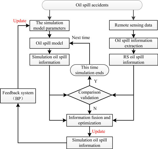
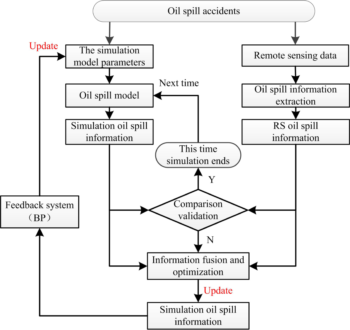
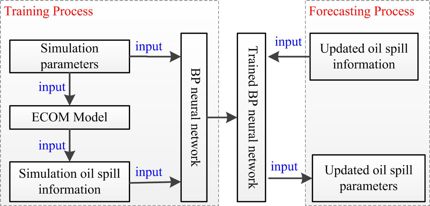
4. DDDAS-Based Oil Spill Simulation

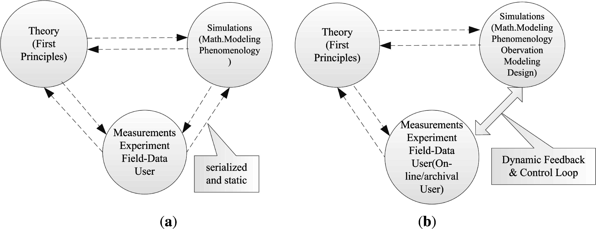
4.1. DDDAS Basic Theory

Traditionally, theory, experiment/test and simulation are separate and conducted in series (Figure 7a). Since large, complex and uncertain systems are generally nonlinear, time-varying and uncertain, it is difficult to establish exact calculations and simulation models [41]. If simulations are combined with experiments or tests, which dynamically incorporate new data, either archival or from online measurements of the actual systems, the application simulations might provide more accurate analysis, more accurate predictions, more precise control and more reliable outcomes (Figure 7b). Based on this idea, Dr. Frederica Darema coined the term dynamic data-driven application systems (DDDAS) around the time she led the organizing effort of the NSF Workshop in March 2000 [19], which opened up a new method for conducting complex system research.
DDDAS is a new paradigm for application simulations and measurements. The simulations receive and respond to online physical data and measurements and/or control the measurements. The DDDAS counterbalances incompleteness in the model and enhances application models by providing additional information to the model, since runtime additional data are used to selectively enhance or refine the original model. The simulations and real systems constitute a symbiotic, operational and dynamic feedback control system [4244].

4.2. DDDAS-Based Oil Spill Simulation

The DDDAS-based ECOM can receive oil slick information extracted from data collected by dynamic remote sensors in the simulation process. Through comparison validation, information fusion and updates, optimized ECOM predictions are obtained; thus, the simulation’s initial parameters are updated. Additionally, this idea also coincides with what has been learned from the rapid response to the Deepwater Horizon oil spill in the Gulf of Mexico: operational oil spill trajectory forecasting should be frequently re-initialized to reduce the forecast errors [2,14]. We then used the updated parameters to calculate more accurate simulation results. The flow chart of the oil spill simulation based on the DDDAS is shown in Figure 8.
Due to the non-linear characteristics of the ECOM, it is difficult to reverse the thinking about the initial conditions and wind field data of the ECOM using the optimized prediction results. In terms of the nonlinear characteristics of artificial neural networks, we chose the BP neural network to back step the initial conditions of the oil spill to optimize the simulation. There are two stages in the BP neural network model: the training process and the forecasting process. At the training stage, ECOM simulation parameters (initial parameters and wind field data included) and simulation results are the input and output parameters of the BP model, respectively; at the forecasting stage, the updated ECOM simulation results are imported into the trained BP neural network, and the output is the updated oil spill initial parameters and wind field data [45,46] (Figure 9).
After four loop iterations, the updated wind field data and simulation initial parameters are as shown in Tables 3 and 4. The overlaid map of the ECOM simulation results and the results extracted from the remote sensors on 11 June are shown in Figure 10.
As can be seen in Figure 10, the oil film extracted from the ASAR image was completely covered by the simulated oil particles, which met our simulation requirements. Then, we entered the next step (14 June) oil spill simulation. After the wind field data from 11 to 13 June was entered, the ECOM simulation was run, and the simulation results for 14 June were generated. Through the BP neural network feedback, the wind field data were updated, and optimized simulated oil particles were obtained. The overlaid map of the ECOM simulation results and the results extracted from the remote sensors on 14 June are shown in Figure 11.
As can be seen in Figure 11, the oil film extracted from the ASAR image was completely covered by the simulated oil particles, and the center points almost overlapped. Therefore, the next oil spill simulation started. As the floating oil was cleaned up by 22 June, taking human intervention into account, the oil simulation dead time was defined by 0:00 a.m. on 20 June. Therefore, we could get the trajectory of the oil particles of 18 consecutive days, from 2 June to 20 June.

5. Validations

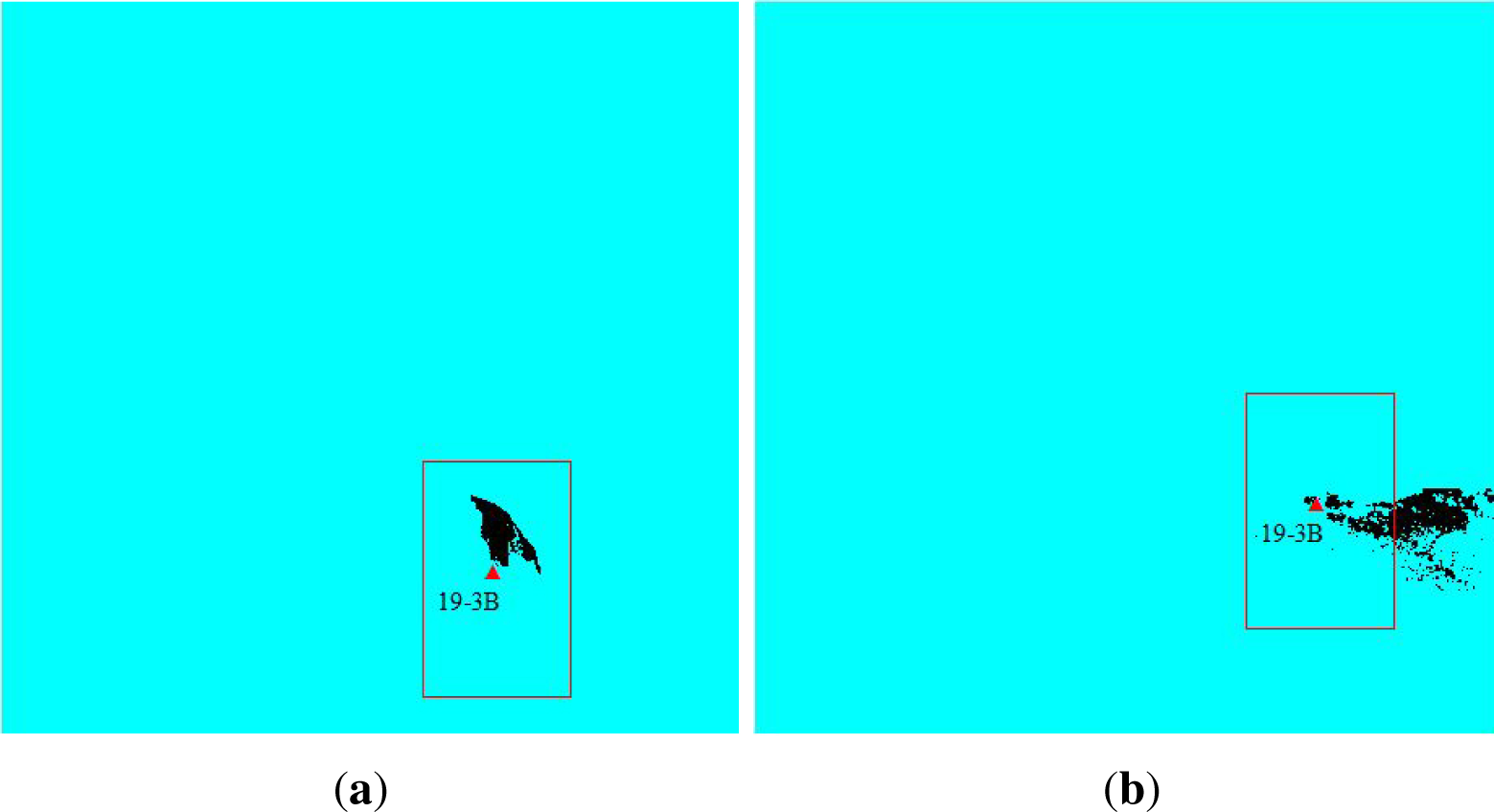
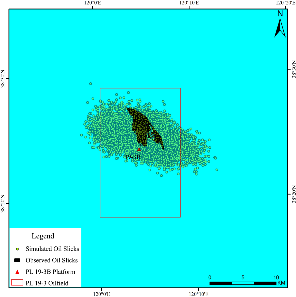
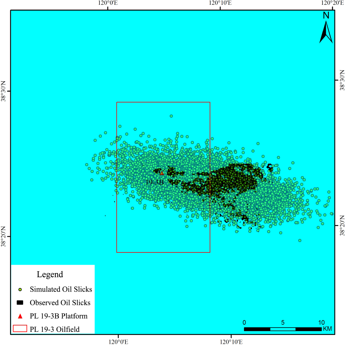
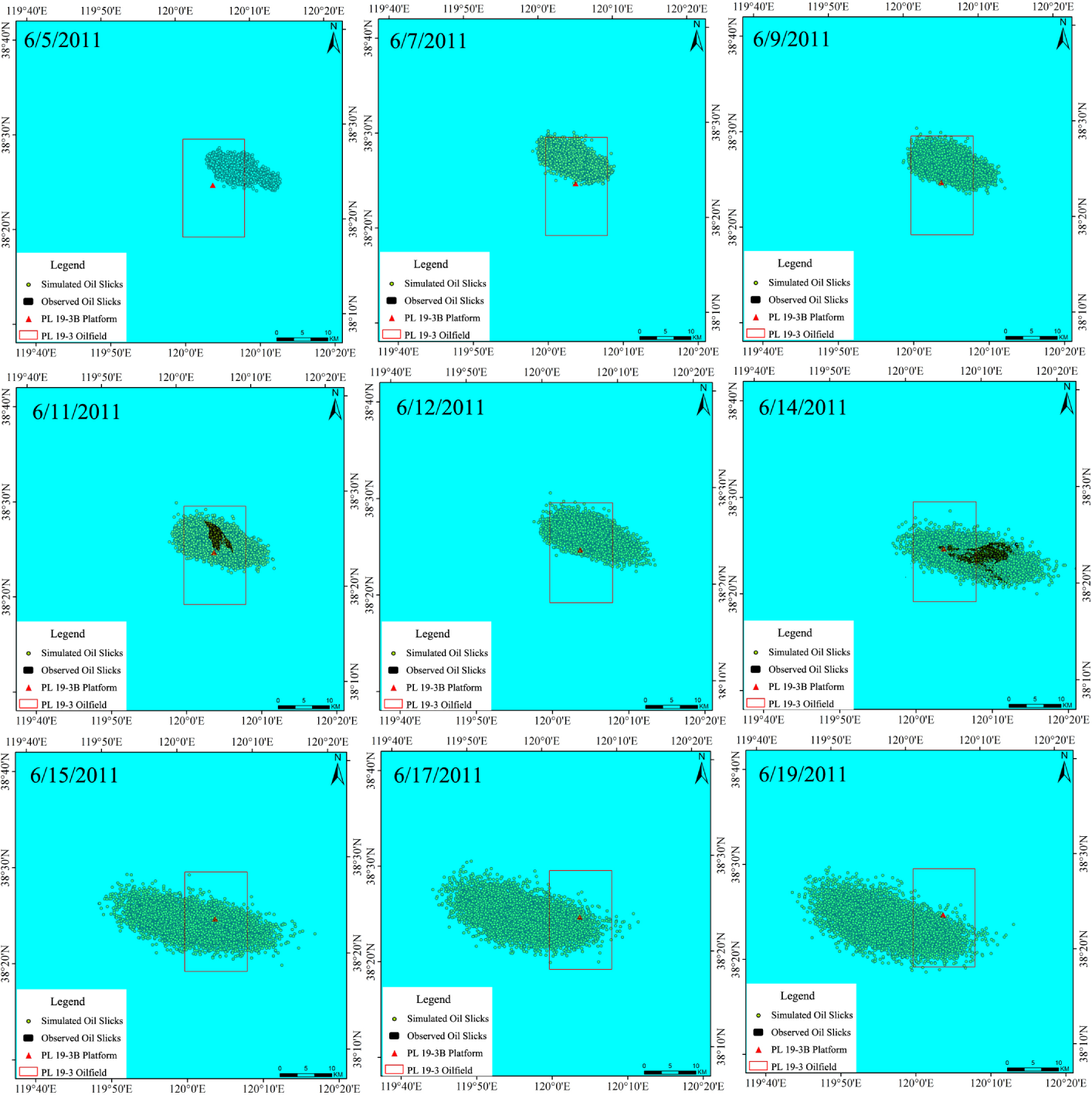
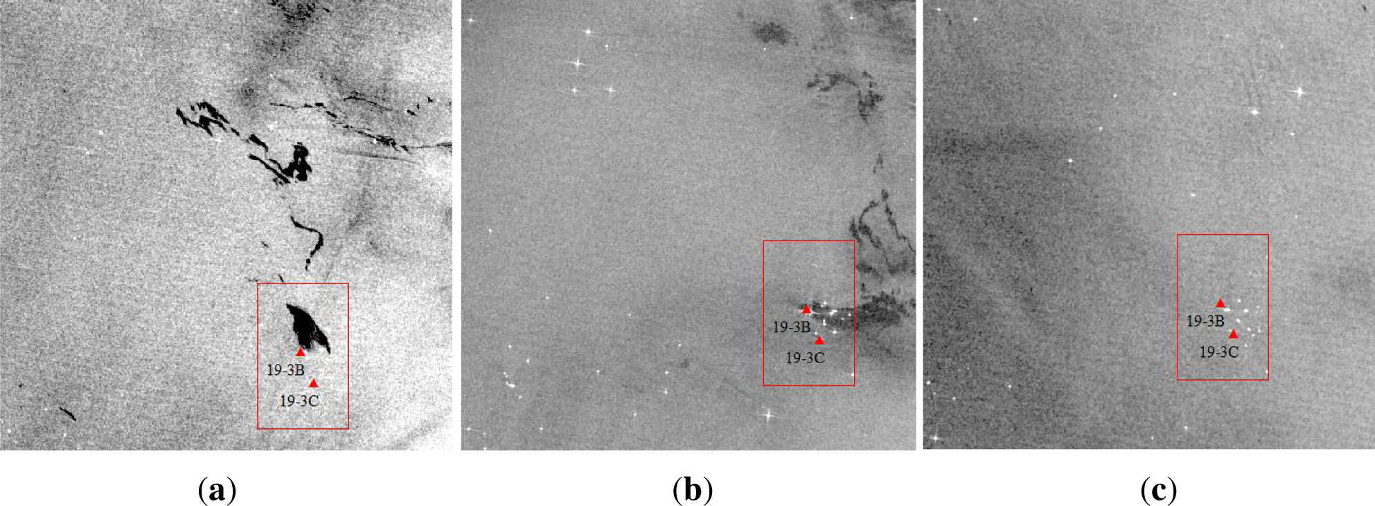
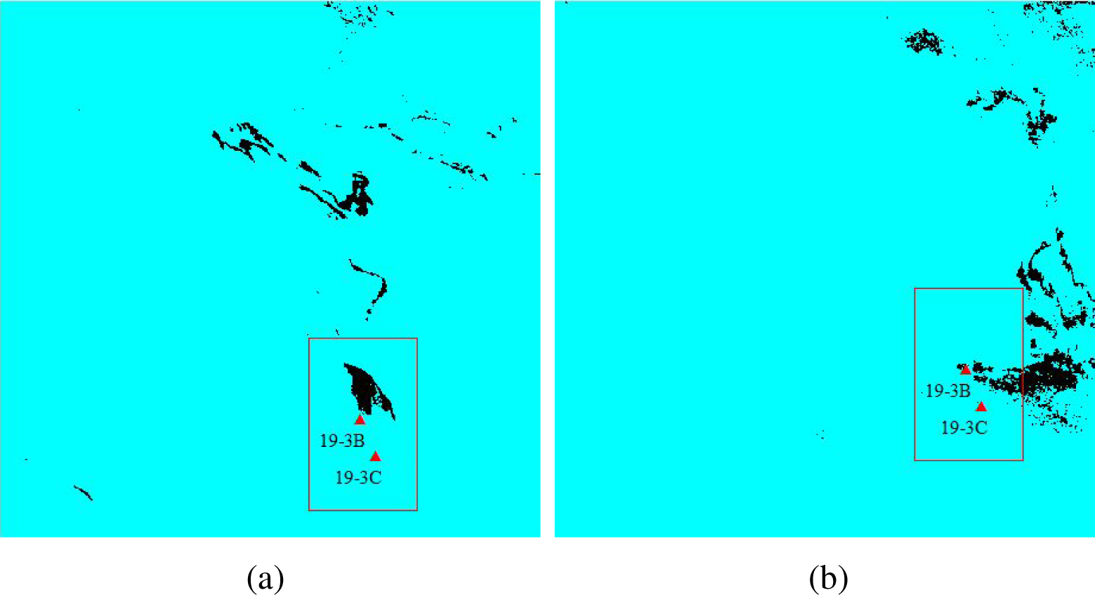
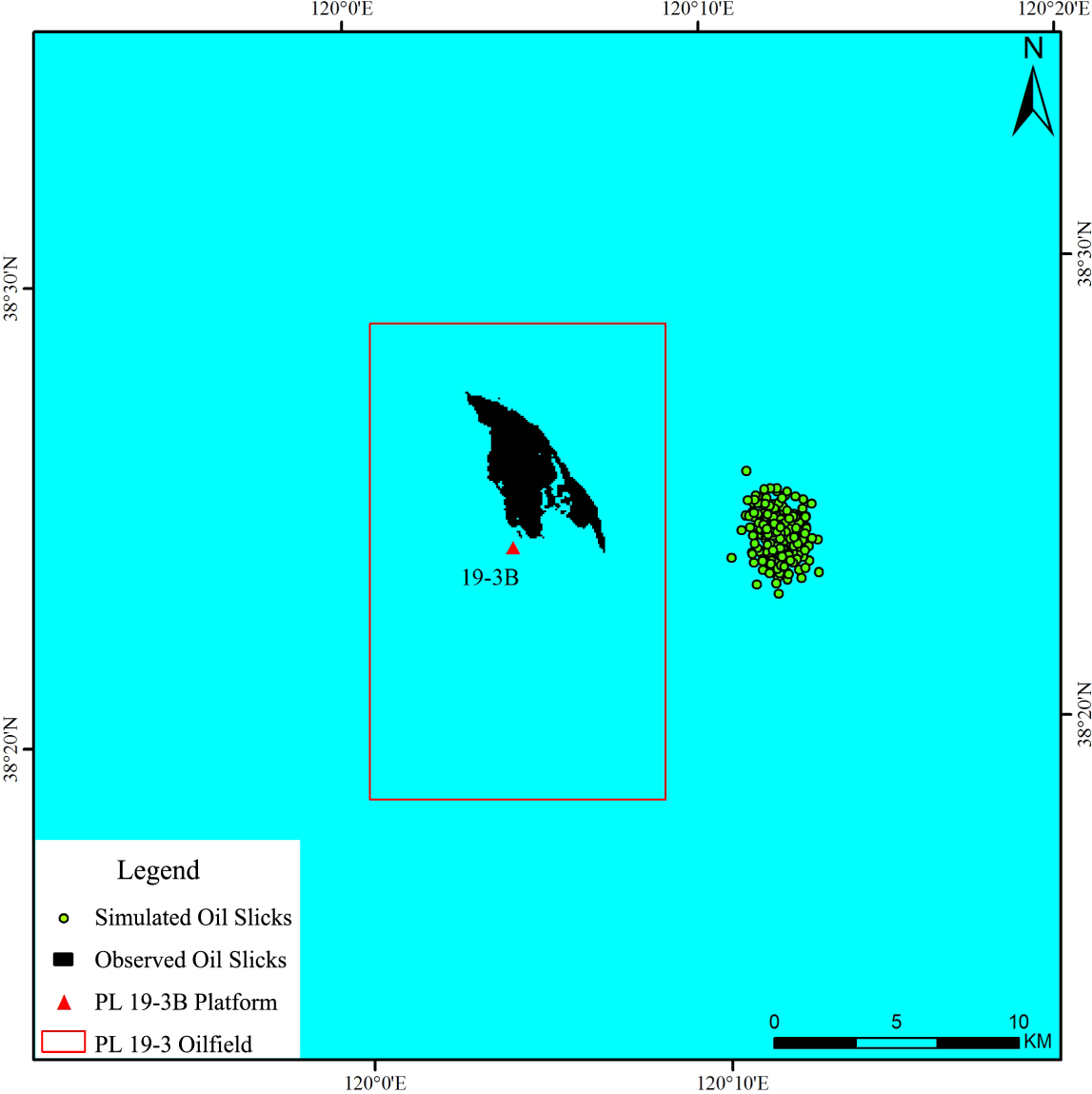
5.1. Penglai Results Validation

Verification of oil spill forecasting is both a crucial issue and a difficult task to perform. In the case of the Penglai 19-3 oil spill, owing to the lack of in situ data, the only way to validate the DDDAS-based ECOM simulation is the comparison between actual oil locations inferred from satellite imagery and the model forecast positions from the latest forecast cycle similar to the work in [14]. In addition, due to the long revisit time for satellites and other reasons, we compared the simulation results with satellite images only by 11 and 14 June 2011. To show vividly the dynamic changing process of oil particles, we also partially listed the simulated trajectory of spilled oil (Figure 12).
As can be seen in Figure 12, a number of simulated oil particles distributed on the northeast of the 19-3B platform on 5 June 2011, which is consistent with the China State Oceanic Administration’s 2011 Bohai Bay Oil Spill Accident Investigation Report: there were amounts of oil film floating on the surface on the northeast of the 19-3B platform on 4 June 2011. Due to the effect of the northwest wind force, particles as simulated mainly tended to transport southeasterly as time progressed. However, affected by the reciprocating flow, as mentioned above, oil particles moved a small distance to the west or north sometimes, as seen in Figure 12 (from 7 to 14 June). In addition, this trajectory of the simulated oil spill could be validated by oil locations inferred from satellite imageries on 11 and 14 June 2011. With the wind speed decreasing and direction changing, as well as the reciprocating flow influence, some simulated oil particles drift towards the west or north, and the overall distribution also became relatively scattered (from 15 to 19 June). This is consistent with the publication by Xu et al. [4].

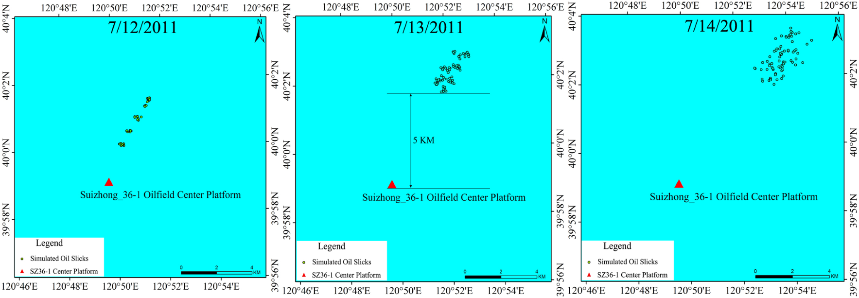
5.2. Other Oil Spill Validation Cases

In addition, in order to further verify the feasibility and practicality of our introduced methodology, we also provided two other oil spill validation cases. The first case was the Dalian Xingang oil spill incident, which happened on 16 July 2010. As the report of the China State Oceanic Administration (SOA) [33], the Dalian Xingang oil spill incident spread an estimated 1500 metric tons of crude oil into the Yellow Sea and stretched over 430 km2 of ocean, with 12 km2 severely affected. Until 26 July, the floating oil was basically cleaned up [3]. Referring to the Penglai 19-3B model setup, we could get the simulated trajectory of spilled oil from 14 to 26 July 2010 (Figure 13), using our introduced methodology. Furthermore, we chose two high-resolution SAR images as the Dalian Xingang monitoring data of the oil spill picked up by remote sensors, obtained on 18 and 21 July 2010. The overlaid map of the ECOM simulation results and the results extracted from the remote sensors on 18 and 21 July are also shown in Figure 13.
As can be seen in Figure 13, a number of simulated oil particles mainly tended to transport southwesterly and northwesterly along the coast as time went on. Additionally, this may be mainly affected by the south and southeast wind force. On 18 and 21 July 2010, the oil films extracted from the SAR images were almost covered by the simulated oil particles; on 19 July 2010, the covered area of the simulated oil film was about 400 km2, calculated using the ArcGIS statistical tool, and this was consistent with the monitoring results of Chinese patrols at 13:30 on 19 July 2010. In a word, using our introduced methodology, the ECOM simulation results of the Dalian Xingang oil spill incident met our simulation requirements.
The second case was the Liaoning Suizhong oil spill incident, which happened on 12 July 2011. It was caused by the control faults of the Suizhong 36-1 oilfield center platform and spread an estimated 0.1 to 0.15 cubic meters of crude oil into the Bohai Sea. According to the 5:00 p.m. report of the Liaoning Suizhong City Office of Emergency Management on 12 July 2011, the crude oil drifted about five kilometers north away from the Suizhong 36-1 oilfield and stretched over 1 km2 of ocean. Until the midday of 13 July, the floating oil was basically cleaned up [33]. Hence, our simulation time span was from 0:00 a.m. on 10 July to 0:00 a.m. on 15 July, and the simulation was based on an assumption that no cleanup was carried out. The simulated trajectory of spilled oil on 12, 13 and 14 July were listed in (Figure 14). Due to the fact that the Liaoning Suizhong oil spill incident was small and it only persisted for one and a half days, we could not find the appropriate remote sensing data to monitor the oil slick’s movement, and the simulation result validation mainly depended on official reports.
As can be seen in Figure 14, the simulated oil particles mainly tended to transport northeasterly as time went on, and the simulated oil film was about five kilometers north away from the Suizhong 36-1 oilfield, which is consistent with the report of the Liaoning Suizhong City Office of Emergency Management.
As a consequence, the two oil spill validation cases have shown the feasibility and practicality of our introduced methodology. However, a lack of sufficient field data at the time of the oil spill event hampered the efforts to validate the oil spill modeling. In the future, it would be good to deploy some surface drifters and validate the modeled trajectory with observations, similar to those in Liu and Weisberg (2011) [47] and Liu et al. (2014) [48].

6. Conclusions

Based on the defect analysis of the oil spill remote sensing and the current oil spill simulation models, the DDDAS was introduced to simulate a marine oil spill. The DDDAS can be viewed as a methodology to counterbalance incompleteness in the model and the capability to enhance the simulation models by imparting additional information into the model, as at runtime, additional data are used to selectively enhance or refine the original model. Combining oil spill data detected by remote sensors with the numerical simulation model, we established an integrated data processing, analysis, forecasting and emergency response system. Taking the oil film extracted from SAR images as the oil spill simulation validation criteria, the initial parameters of the simulation model were updated. Therefore, the prediction accuracy of the simulation model increased, and the error caused by empirical parameters reduced in existing simulation systems.
The Penglai, Xingang and Suizhong oil spill results showed that the DDDAS-based simulation system had good predictive capacity. That is to say, our oil spill simulation system could dynamically incorporate oil slick information extracted from remote sensing data, and the application simulations could offer the promise of more accurate analysis, more accurate predictions, more precise controls and more reliable outcomes. This system can effectively improve oil spill simulation and diffusion forecasting and improve decision making during marine oil spill emergencies.
For the ECOM model, we emphasize tidal currents and wind as dominant driving forces; wave-induced currents were ignored during simulations. However, some literature suggests that adding wave effects in ocean model systems is likely to increase the predictability of surface drifter trajectories [49]. Therefore, adding wave effects in simulations and obtaining more accurate simulation results require further study. Furthermore, due to the scarcity of in situ data, a sensitivity analysis or a skill score could not be performed. As a consequence, some future work, such as more extensive model validations [47,48] and multiple model ensembles [2,14], should be done.

Acknowledgments

Dr. Lizhe Wang’s work is supported by the National High Technology Research and Development Program of China (“863” Program) (No. 2013AA12A301). The authors would also like to acknowledge the editors and anonymous reviewers for their valuable comments on the manuscript.

Author Contributions

Jining Yan and Lizhe Wang developed the oil spill detection and simulation methodology, its relative software, as well as the main part of the present manuscript. Lajiao Chen, Lingjun Zhao and Bormin Huang participated in the methodology development on the basis of their previous research in oil spill detection and simulation.

Conflicts of Interest

The authors declare no conflict of interest.

References

  1. Li, Y.; Wang, L.; Chen, L.; Ma, Y.; Zhu, X.; Chu, B. Application of DDDAS in Marine Oil Spill Management: A New Framework Combining Multiple Source Remote Sensing Monitoring and Simulation as a Symbiotic Feedback Control System. Proceedings of the 2013 33rd IEEE International Geoscience and Remote Sensing Symposium (IGARSS), Melbourne, Australia, 21–26 July 2013; pp. 4526–4529.
  2. Liu, Y.; Weisberg, R.H.; Hu, C.; Zheng, L. Tracking the Deepwater Horizon oil spill: A modeling perspective. Eos Trans. Am. Geophys. Union 2011, 92, 45–46. [Google Scholar]
  3. Lv, Y.; Zhang, W.; Gao, Y.; Ning, S.; Yang, B. Preliminary study on responses of marine nematode community to crude oil contamination in intertidal zone of Bathing Beach, Dalian. Mar. Pollut. Bull 2011, 62, 2700–2706. [Google Scholar]
  4. Xu, Q.; Li, X.; Wei, Y.; Tang, Z.; Cheng, Y.; Pichel, W.G. Satellite observations and modeling of oil spill trajectories in the Bohai Sea. Mar. Pollut. Bull 2013, 71, 107–116. [Google Scholar]
  5. Leifer, I.; Lehr, W.J.; Simecek-Beatty, D.; Bradley, E.; Clark, R.; Dennison, P.; Hu, Y.; Matheson, S.; Jones, C.E.; Holt, B.; et al. State of the art satellite and airborne marine oil spill remote sensing: Application to the BP Deepwater Horizon oil spill. Remote Sens. Environ 2012, 124, 185–209. [Google Scholar]
  6. Fingas, M.; Brown, C. Review of oil spill remote sensing. Mar. Pollut. Bull 2014, 83, 9–23. [Google Scholar]
  7. Plaza, J.; Pérez, R.; Plaza, A.; Martínez, P.; Valencia, D. Mapping oil spills on sea water using spectral mixture analysis of hyperspectral image data. Proc. SPIE 2005, 5995. [Google Scholar] [CrossRef]
  8. Ivanov, A.Y.; Zatyagalova, V.V. A GIS approach to mapping oil spills in a marine environment. Int. J. Remote Sens 2008, 29, 6297–6313. [Google Scholar]
  9. Jha, M.N.; Levy, J.; Gao, Y. Advances in remote sensing for oil spill disaster management: state-of-the-art sensors technology for oil spill surveillance. Sensors 2008, 8, 236–255. [Google Scholar]
  10. Pisano, A.; Bignami, F.; Santoleri, R. Oil Spill Detection in Glint-Contaminated Near-Infrared MODIS Imagery. Remote Sens 2015, 7, 1112–1134. [Google Scholar]
  11. Ramsey, E., III; Rangoonwala, A.; Suzuoki, Y.; Jones, C.E. Oil detection in a coastal marsh with polarimetric synthetic aperture radar (SAR). Remote Sens 2011, 3, 2630–2662. [Google Scholar]
  12. Ventikos, N.P.; Vergetis, E.; Psaraftis, H.N.; Triantafyllou, G. A high-level synthesis of oil spill response equipment and countermeasures. J. Hazard. Mater 2004, 107, 51–58. [Google Scholar]
  13. Azevedo, A.; Oliveira, A.; Fortunato, A.; Bertin, X. Application of an Eulerian-Lagrangian oil spill modeling system to the Prestige accident: trajectory analysis. J. Coast. Res 2009, 1, 777–781. [Google Scholar]
  14. Liu, Y.; Weisberg, R.H.; Hu, C.; Zheng, L. Trajectory forecast as a rapid response to the Deepwater Horizon oil spill. In Monitoring and Modeling the Deepwater Horizon Oil Spill: A Record-Breaking Enterprise; Elsevier: Amsterdam, The Netherlands, 2011; pp. 153–165. [Google Scholar]
  15. Liu, Y.; MacFadyen, A.; Ji, Z.G.; Weisberg, R.H. (Eds.) Monitoring and Modeling the Deepwater Horizon Oil Spill: A Record Breaking Enterprise. In Geophysical Monograph Series; American Geophysical Union: Washington, DC, USA, 2011; Volume 195, pp. 1–271.
  16. Zodiatis, G.; Lardner, R.; Solovyov, D.; Panayidou, X.; de Dominicis, M. Predictions for oil slicks detected from satellite images using MyOcean forecasting data. Ocean Sci 2012, 8, 1105–1115. [Google Scholar] [Green Version]
  17. De Dominicis, M.; Pinardi, N.; Zodiatis, G.; Archetti, R. MEDSLIK-II, a Lagrangian marine surface oil spill model for short-term forecasting—Part 2: Numerical simulations and validations. Geosci. Model Dev 2013, 6, 1871–1888. [Google Scholar]
  18. Elhakeem, A.; Elshorbagy, W.; Chebbi, R. Oil spill simulation and validation in the Arabian (Persian) Gulf with special reference to the UAE coast. Water Air Soil Pollut 2007, 184, 243–254. [Google Scholar]
  19. Darema, F. Dynamic data driven applications systems: A new paradigm for application simulations and measurements. Proceeding the 4th International Conference on Computational Science-ICCS 2004, Kraków, Poland, 6–9 June 2004; pp. 662–669.
  20. Hu, C.; Müller-Karger, F.E.; Taylor, C.J.; Myhre, D.; Murch, B.; Odriozola, A.L.; Godoy, G. MODIS detects oil spills in Lake Maracaibo, Venezuela. Eos Trans. Am. Geophys. Union 2003, 84, 313–319. [Google Scholar]
  21. Migliaccio, M.; Nunziata, F.; Brown, C.E.; Holt, B.; Li, X.; Pichel, W.; Shimada, M. Polarimetric synthetic aperture radar utilized to track oil spills. Eos Trans. Am. Geophys. Union 2012, 93, 161–162. [Google Scholar]
  22. Zhang, Y.; Li, Y.; Lin, H. Oil-Spill pollution remote sensing by Synthetic Aperture Radar. In Advanced Geoscience Remote Sensing; InTech: Rijeka, Croatia, 2014; pp. 27–50. [Google Scholar]
  23. Amoon, M.; Bozorgi, A.; Rezai-rad, G.A. New method for ship detection in synthetic aperture radar imagery based on the human visual attention system. J. Appl. Remote Sens 2013, 7. [Google Scholar] [CrossRef]
  24. Brekke, C.; Solberg, A.H. Classifiers and confidence estimation for oil spill detection in ENVISAT ASAR images. IEEE Geosci. Remote Sens. Lett 2008, 5, 65–69. [Google Scholar]
  25. Marghany, M.; Cracknell, A.P.; Hashim, M. Comparison between radarsat-1 SAR different data modes for oil spill detection by a fractal box counting algorithm. Int. J. Digit. Earth 2009, 2, 237–256. [Google Scholar]
  26. Li, X.; Li, C.; Yang, Z.; Pichel, W. SAR imaging of ocean surface oil seep trajectories induced by near inertial oscillation. Remote Sens. Environ 2013, 130, 182–187. [Google Scholar]
  27. Brekke, C.; Solberg, A.H. Oil spill detection by satellite remote sensing. Remote Sens. Environ 2005, 95, 1–13. [Google Scholar]
  28. Shirvany, R.; Chabert, M.; Tourneret, J.Y. Ship and oil-spill detection using the degree of polarization in linear and hybrid/compact dual-pol SAR. IEEE J. Sel. Top. Appl. Earth Obs. Remote Sens 2012, 5, 885–892. [Google Scholar]
  29. Lu, Y.; Tian, Q.; Wang, X.; Zheng, G.; Li, X. Determining oil slick thickness using hyperspectral remote sensing in the Bohai Sea of China. Int. J. Digit. Earth 2013, 6, 76–93. [Google Scholar]
  30. Liu, X.; Guo, J.; Guo, M.; Hu, X.; Tang, C.; Wang, C.; Xing, Q. Modelling of oil spill trajectory for 2011 Penglai 19-3 coastal drilling field, China. Appl. Math. Model 2014. [Google Scholar] [CrossRef]
  31. Liu, P.; Huang, F.; Li, G.; Liu, Z. Remote-Sensing image denoising using partial differential equations and auxiliary images as priors. IEEE. Geosci. Remote Sens. Lett 2012, 3, 358–362. [Google Scholar]
  32. Liu, P.; Eom, K.B. Restoration of multispectral images by total variation with auxiliary image. Opt. Lasers Eng 2013, 7, 873–882. [Google Scholar]
  33. The China State Oceanic Administration, 2011 Bohai Bay Oil Spill Accident Investigation Report by the Joint Investigation Team; The China State Oceanic Administration: Beijing, China, 2011; in Chinese.
  34. Ganta, R.R.; Zaheeruddin, S.; Baddiri, N.; Rao, R. Segmentation of oil spill images with illumination-reflectance based adaptive level set model. IEEE J. Sel. Top. Appl. Earth Obs. Remote Sens 2012, 5, 1394–1402. [Google Scholar]
  35. Moctezuma, M.; Parmiggiani, F. Adaptive stochastic minimization for measuring marine oil spill extent in synthetic aperture radar images. J. Appl. Remote Sens 2014, 8, 083553. [Google Scholar]
  36. Chaudhuri, D.; Samal, A.; Agrawal, A.; Mishra, A.; Gohri, V.; Agarwal, R.; et al. A statistical approach for automatic detection of ocean disturbance features from SAR images. IEEE J. Sel. Top. Appl. Earth Obs. Remote Sens 2012, 5, 1231–1242. [Google Scholar]
  37. Blumberg, A.F.; Mellor, G.L. A description of a three-dimensional coastal ocean circulation model. In Three-Dimensional Coastal Ocean Models; American Geophysical Union: Washington, DC, USA, 1987; pp. 1–16. [Google Scholar]
  38. Guo, J.; Liu, X.; Xie, Q. Characteristics of the Bohai Sea oil spill and its impact on the Bohai Sea ecosystem. Chin. Sci. Bull 2013, 58, 2276–2281. [Google Scholar]
  39. Tkalich, P.; Chan, E.S. Vertical mixing of oil droplets by breaking waves. Mar. Pollut. Bull 2002, 44, 1219–1229. [Google Scholar]
  40. Mu, L.; Wu, S.; Song, J.; Li, H.; Liu, S.; Li, Y.; Gao, J. Numerical model research on Emergency Warning & Predicting system of ocean oil spill: I. Research on predicting of ocean dynamical factors. Mar. Sci. Bull 2011, 5, 502–508, in Chinese. [Google Scholar]
  41. Denham, M.; Cortés, A.; Margalef, T.; Luque, E. Applying a dynamic data driven genetic algorithm to improve forest fire spread prediction. Proseedings of the Computational Science—ICCS 2008, Kraków, Poland, June 23–25 2008; pp. 36–45.
  42. Madey, G.R.; Barabási, A.; Chawla, N.V.; Gonzalez, M.; Hachen, D.; Lantz, B.; Pawling, A.; Schoenharl, T.; Szabó, G.; Wang, P.; et al. Enhanced situational awareness: Application of DDDAS concepts to emergency and disaster management. Proseedings of the Computational Science—ICCS 2007, Beijing, China, 27–30 May 2007.
  43. Darema, F. Dynamic data driven applications systems: New capabilities for application simulations and measurements. Proseedings of the Computational Science—ICCS 2005, Atlanta, GA, USA, 22–25 May 2005; pp. 610–615.
  44. Wang, L.; Chen, D.; Liu, W.; Ma, Y.; Wu, Y.; Deng, Z. DDDAS-Based Parallel Simulation of Threat Management for Urban Water Distribution Systems. Comput. Sci. Eng 2014, 16, 8–17. [Google Scholar]
  45. Garcia-Pineda, O.; MacDonald, I.R.; Li, X.; Jackson, C.R.; Pichel, W.G. Oil spill mapping and measurement in the Gulf of Mexico with Textural Classifier Neural Network Algorithm (TCNNA). IEEE J. Sel. Top. Appl. Earth Obs. Remote Sens 2013, 6, 2517–2525. [Google Scholar]
  46. Topouzelis, K.; Karathanassi, V.; Pavlakis, P.; Rokos, D. Dark formation detection using neural networks. Int. J. Remote Sens 2008, 29, 4705–4720. [Google Scholar]
  47. Liu, Y.; Weisberg, R.H. Evaluation of trajectory modeling in different dynamic regions using normalized cumulative Lagrangian separation. J. Geophys. Res.: Oceans 2011, 116, C09013. [Google Scholar]
  48. Liu, Y.; Weisberg, R.H.; Vignudelli, S.; Mitchum, G.T. Evaluation of altimetry-derived surface current products using Lagrangian drifter trajectories in the eastern Gulf of Mexico. J. Geophys. Res.: Oceans 2014, 119, 2827–2842. [Google Scholar]
  49. Röhrs, J.; Christensen, K.H.; Hole, L.R.; Broström, G.; Drivdal, M.; Sundby, S. Observation-based evaluation of surface wave effects on currents and trajectory forecasts. Ocean Dyn 2012, 62, 1519–1533. [Google Scholar]
Figure 1. The location of Penglai 19-3 Oilfield and Penglai19-3B, C Platform.
Remotesensing 07 07105f1
Figure 2. ASAR images of Penglai 19-3 Oilfield: (a) 11 June 2011; (b) 14 June 2011; (c) 22 June 2011.
Remotesensing 07 07105f2
Figure 3. ASAR images’ histograms: (a) 11 June 2011; (b) 14 June 2011.
Remotesensing 07 07105f3
Figure 4. Oil spill information extracted results: (a) 11 June 2011; (b) 14 June 2011.
Remotesensing 07 07105f4
Figure 5. Oil film for ECOM simulation: (a) 11 June 2011; (b) 14 June 2011.
Remotesensing 07 07105f5
Figure 6. 11 June 2011 overlaid map of simulation results and RS extraction results.
Remotesensing 07 07105f6
Figure 7. Traditional mode and DDDAS theory: (a) traditional mode (b) DDDAS.
Remotesensing 07 07105f7
Figure 8. DDDAS-based oil spill simulation.
Remotesensing 07 07105f8
Figure 9. BP feedback system.
Remotesensing 07 07105f9
Figure 10. 11 June 2011 overlaid map of final simulation results and RS extraction results.
Remotesensing 07 07105f10
Figure 11. 14 June 2011 overlaid map of final simulation results and RS extraction results.
Remotesensing 07 07105f11
Figure 12. Trajectories of the Penglai 19-3B simulated oil spills.
Remotesensing 07 07105f12
Figure 13. Trajectories of the Dalian Xingang simulated oil spills.
Remotesensing 07 07105f13
Figure 14. Trajectories of the Liaoning Suizhong simulated oil spills.
Remotesensing 07 07105f14
Table 1. Wind field data for the Estuarine and Coastal Ocean Model (ECOM) simulation (part).
Time (h)Wind Speed (m/s)Wind Direction (°)
545112.5
571247.5
601247.5
633315
662112.5
69190.0
72390.0
754112.5
787180.0
814157.5
845180.0
874202.5
904157.5
935157.5
Table 2. Initial parameters of the ECOM simulation.
Initial ParametersInitial Values
Oil spilling point X93
Oil spilling point Y52
Step size30
Oil particles number100
Start step961
End step7860
Table 3. Updated wind field data for ECOM simulation (part).
Time (h)Updated Wind Speed (m/s)Updated Wind Direction (°)
544220.0
573347.5
605312.5
634210.0
666120.0
69390.0
725140.0
757242.5
789337.5
816210.5
848270.0
876270.5
907320.5
938315.0
Table 4. Updated parameters for ECOM simulation.
Updated ParametersUpdated Values
Oil spilling point X91
Oil spilling point Y54
Step size30
Oil particles Number100
Start step961
End step4320

