
Advancing of Land Surface Temperature Retrieval Using Extreme Learning Machine and Spatio-Temporal Adaptive Data Fusion Algorithm


Abstract
:
1. Introduction
2. Methodology
2.1. Extreme Learning Machine (ELM) Algorithm
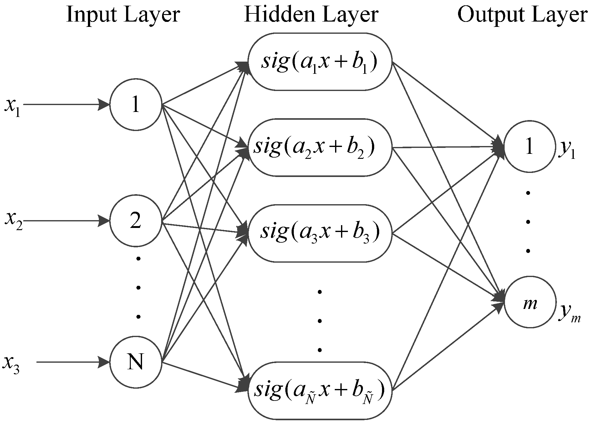
- (i)
- Allocate the input weight and bias arbitrarily.
- (ii)
- Compute the hidden layer output matrix .
- (iii)
- Use the equation to calculate the output weight matrix .
2.2. Spatio-Temporal Adaptive Data Fusion Algorithm for Temperature Mapping (SADFAT)
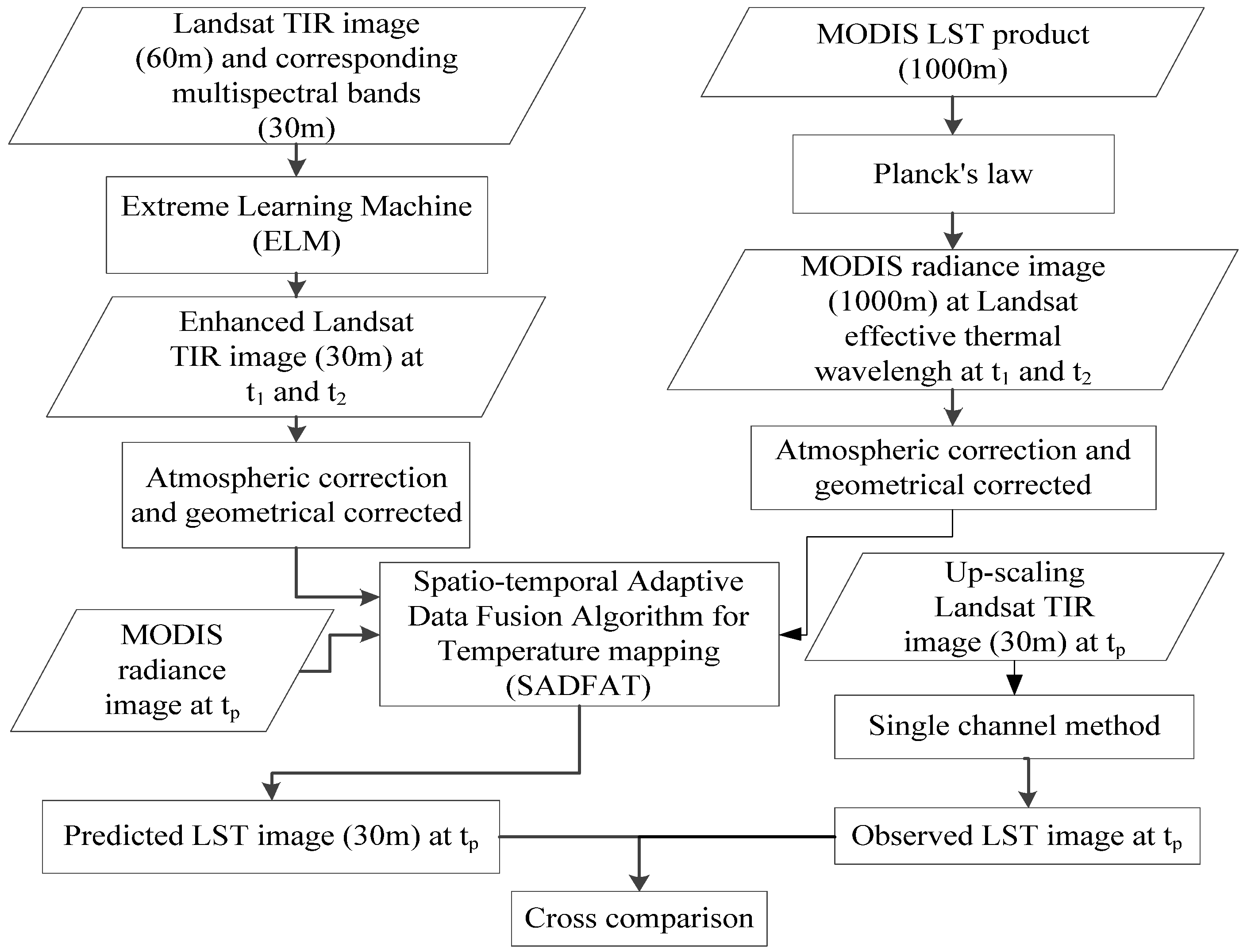
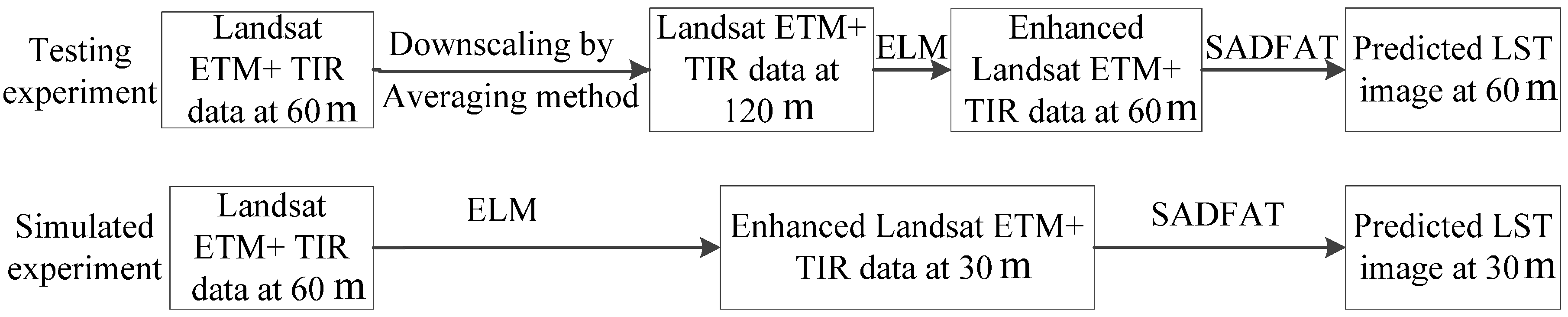
2.3. Implementation of the Proposed Data Fusion Model
- (i)
- Two L images were used to search for the spectrally similar pixels using the method described by Gao et al. [34] that define a difference threshold between the central pixel and the neighbouring pixels in a moving window.
- (ii)
- The combined weight and conversion coefficient for each similar pixel were computed. Here, a similar pixel with higher thermal similarity and shorter distance to the central pixel would yield a higher weight and the conversion coefficients were decided by the regression analysis of the similar pixels [35].
- (iii)
- Equation (5) was employed to compute the desired predicted image at tp. Considering the temporal weights of the two images given by the temporal changes in coarser radiance images, an accurate radiance image can be computed by using the weighted combination of the two predicted radiance images as follows:where represents a location of the central pixel in a moving window, t is the acquisition date, and are the predicted radiance image using L image at t1 and t2 as the base image, respectively, in which the temporal weight Tk can be calculated as:where M(x, y, t, B) is the resampled radiance at time t of band B.
- (iv)
- Finally, the LST images can be derived using the generalized single channel method.

3. Results
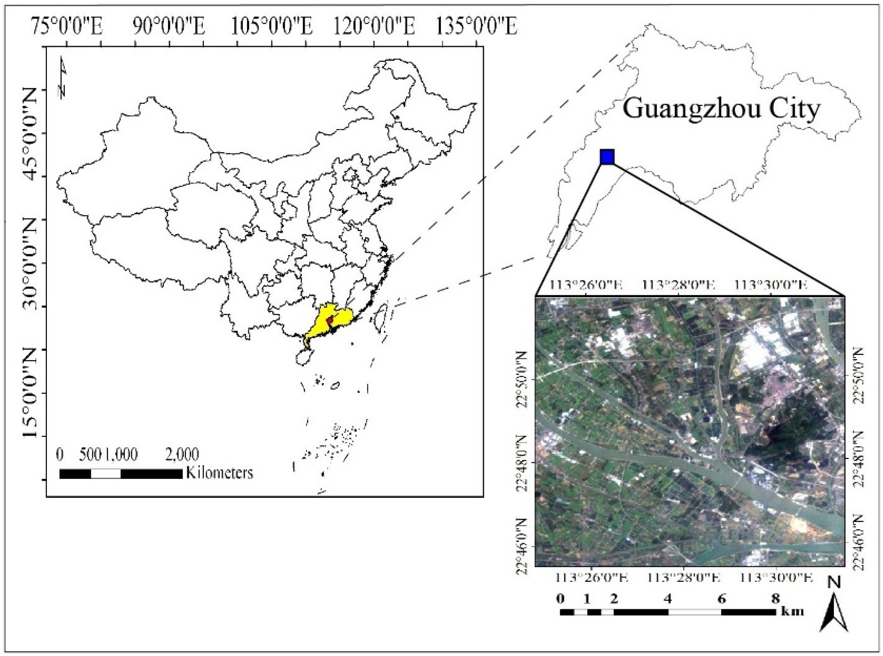
3.1. Study Area
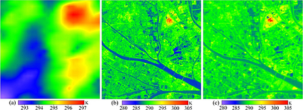
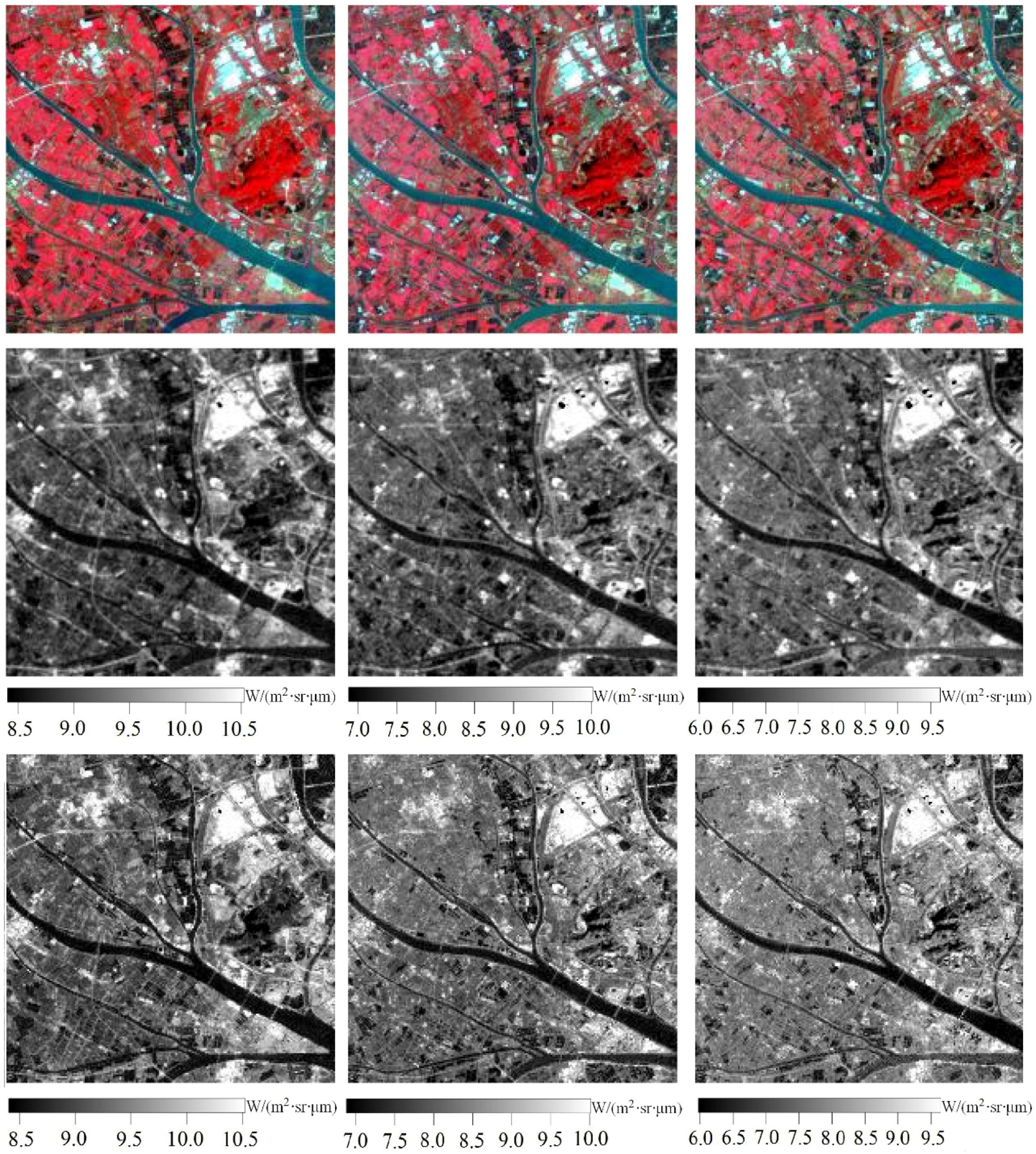
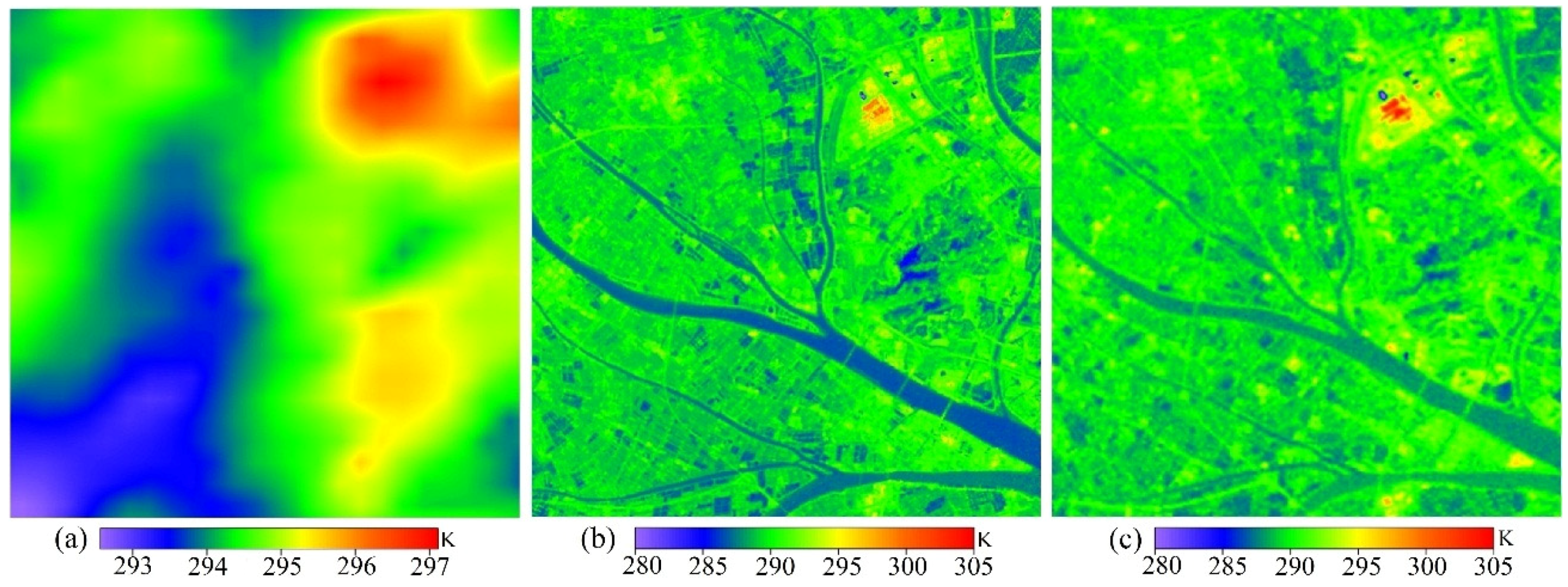
3.2. Experiment Results


| Date | 20 October 2013 | 7 December 2013 | 23 December 2013 |
|---|---|---|---|
| CC | 0.8788 * | 0.8251 * | 0.8017 * |
| RMSE | 0.0844 | 0.0891 | 0.0909 |
| AD | −9.8940e-06 | −2.1980e-06 | 6.3913e-06 |
| AAD | 0.0595 | 0.0620 | 0.0614 |


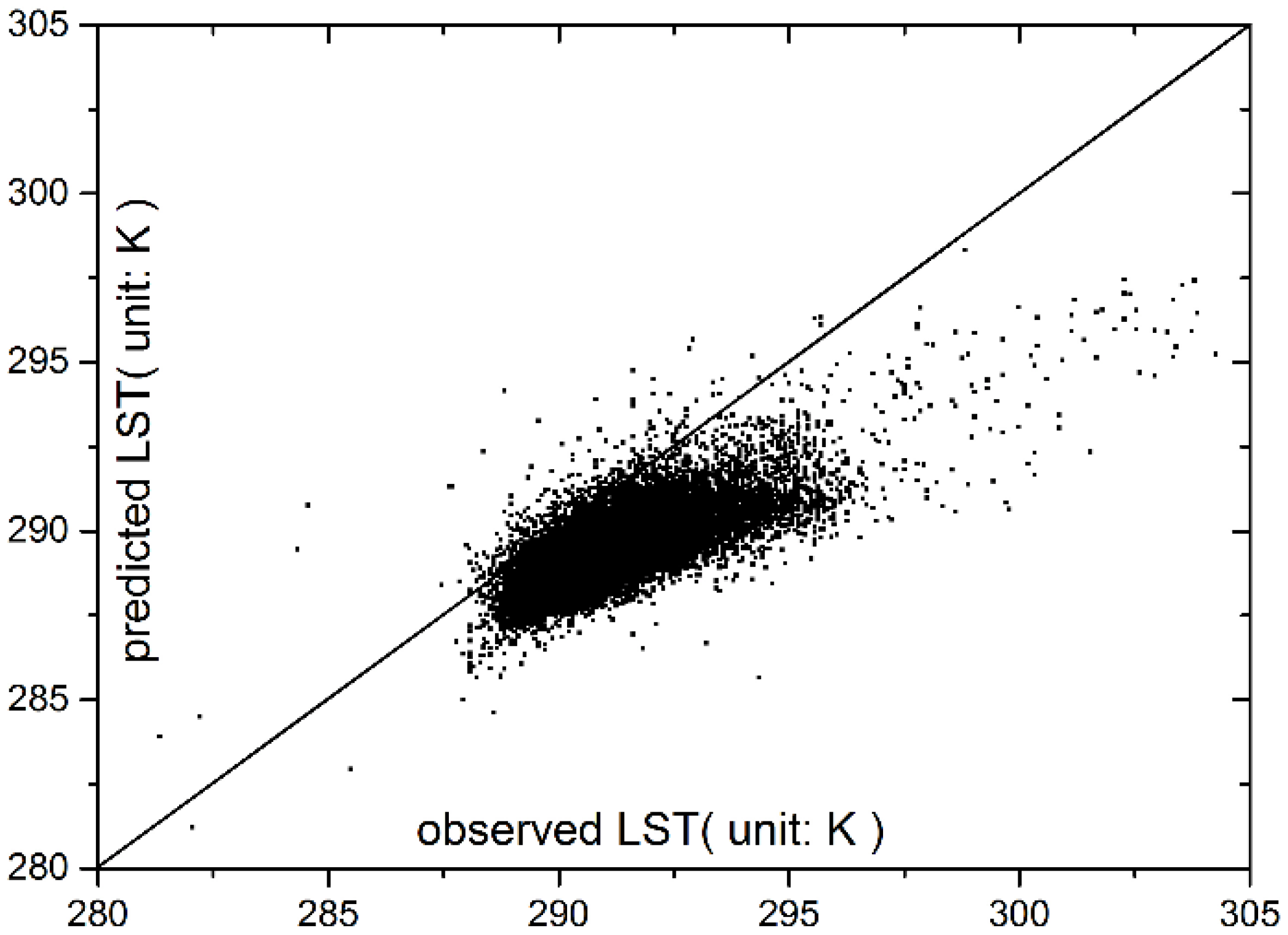
| Indicator | CC | RMSE | AD | AAD |
|---|---|---|---|---|
| testing experiment | 0.7554 * | 1.8242 | 1.6354 | 1.6498 |
4. Discussion
5. Conclusion
Acknowledgments
Author Contributions
Appendix A. Extreme Learning Machine (ELM) Algorithm
Appendix B. Spatio-Temporal Adaptive Data Fusion Algorithm for Temperature Mapping (SADFAT)
Conflicts of Interest
References
- Kalma, J.D.; McVicar, T.R.; McCabe, M.F. Estimating land surface evaporation: A review of methods using remotely sensed surface temperature data. Surveys Geophys. 2008, 29, 421–469. [Google Scholar] [CrossRef]
- Cammalleri, C.; Anderson, M.; Ciraolo, G.; D’Urso, G.; Kustas, W.; La Loggia, G.; Minacapilli, M. Applications of a remote sensing-based two-source energy balance algorithm for mapping surface fluxes without in situ air temperature observations. Remote Sens. Environ. 2012, 124, 502–515. [Google Scholar] [CrossRef]
- Srivastava, P.K.; Han, D.; Ramirez, M.R.; Islam, T. Machine learning techniques for downscaling smos satellite soil moisture using modis land surface temperature for hydrological application. Water Resour. Manag. 2013, 27, 3127–3144. [Google Scholar] [CrossRef]
- Song, X.; Leng, P.; Li, X.; Li, X.; Ma, J. Retrieval of daily evolution of soil moisture from satellite-derived land surface temperature and net surface shortwave radiation. Int. J. Remote Sens. 2013, 34, 3289–3298. [Google Scholar] [CrossRef]
- Bateni, S.; Entekhabi, D.; Castelli, F. Mapping evaporation and estimation of surface control of evaporation using remotely sensed land surface temperature from a constellation of satellites. Water Resour. Res. 2013, 49, 950–968. [Google Scholar] [CrossRef]
- Tang, R.; Li, Z.-L.; Jia, Y.; Li, C.; Chen, K.-S.; Sun, X.; Lou, J. Evaluating one-and two-source energy balance models in estimating surface evapotranspiration from Landsat-derived surface temperature and field measurements. Int. J. Remote Sens. 2013, 34, 3299–3313. [Google Scholar] [CrossRef]
- Anderson, M.; Kustas, W.; Norman, J.; Hain, C.; Mecikalski, J.; Schultz, L.; González-Dugo, M.; Cammalleri, C.; D’Urso, G.; Pimstein, A. Mapping daily evapotranspiration at field to continental scales using geostationary and polar orbiting satellite imagery. Hydrol. Earth Syst. Sci. 2011, 15, 223–239. [Google Scholar] [CrossRef] [Green Version]
- Wong, M.S.; Nichol, J.E. Spatial variability of frontal area index and its relationship with urban heat island intensity. Int. J. Remote Sens. 2013, 34, 885–896. [Google Scholar] [CrossRef]
- Weng, Q.; Fu, P. Modeling annual parameters of clear-sky land surface temperature variations and evaluating the impact of cloud cover using time series of landsat tir data. Remote Sens. Environ. 2014, 140, 267–278. [Google Scholar] [CrossRef]
- Goward, S.N.; Masek, J.G.; Williams, D.L.; Irons, J.R.; Thompson, R. The landsat 7 mission: Terrestrial research and applications for the 21st century. Remote Sens. Environ. 2001, 78, 3–12. [Google Scholar] [CrossRef]
- Anderson, M.C.; Allen, R.G.; Morse, A.; Kustas, W.P. Use of landsat thermal imagery in monitoring evapotranspiration and managing water resources. Remote Sens. Environ. 2012, 122, 50–65. [Google Scholar] [CrossRef]
- Almeida, T.; de Souza Filho, C.; Rossetto, R. Aster and landsat ETM+ images applied to sugarcane yield forecast. Int. J. Remote Sens. 2006, 27, 4057–4069. [Google Scholar] [CrossRef]
- Sameen, M.I.; Al Kubaisy, M.A. Automatic surface temperature mapping in arcgis using landsat-8 tirs and envi tools, case study: Al Habbaniyah Lake. J. Environ. Earth Sci. 2014, 4, 12–17. [Google Scholar]
- Li, Y.-Y.; Zhang, H.; Kainz, W. Monitoring patterns of urban heat islands of the fast-growing shanghai metropolis, china: Using time-series of landsat tm/etm+ data. Int. J. Appl. Earth Obs. Geoinf. 2012, 19, 127–138. [Google Scholar] [CrossRef]
- Masek, J.G.; Collatz, G.J. Estimating forest carbon fluxes in a disturbed southeastern landscape: Integration of remote sensing, forest inventory, and biogeochemical modeling. J. Geophys. Res. 2006, 111. [Google Scholar] [CrossRef]
- Ju, J.; Roy, D.P. The availability of cloud-free landsat ETM+ data over the conterminous united states and globally. Remote Sens. Environ. 2008, 112, 1196–1211. [Google Scholar] [CrossRef]
- Leckie, D.G. Advances in remote sensing technologies for forest surveys and management. Can. J. For. Res. 1990, 20, 464–483. [Google Scholar] [CrossRef]
- Justice, C.O.; Vermote, E.; Townshend, J.R.; Defries, R.; Roy, D.P.; Hall, D.K.; Salomonson, V.V.; Privette, J.L.; Riggs, G.; Strahler, A. The moderate resolution imaging spectroradiometer (modis): Land remote sensing for global change research. IEEE Trans. Geosci. Remote Sens. 1998, 36, 1228–1249. [Google Scholar] [CrossRef]
- Stathopoulou, M.; Cartalis, C. Downscaling avhrr land surface temperatures for improved surface urban heat island intensity estimation. Remote Sens. Environ. 2009, 113, 2592–2605. [Google Scholar] [CrossRef]
- Pohl, C.; Van Genderen, J. Review article multisensor image fusion in remote sensing: Concepts, methods and applications. Int. J. Remote Sens. 1998, 19, 823–854. [Google Scholar] [CrossRef]
- Smith, M.I.; Heather, J.P. A review of image fusion technology in 2005. In Defense and Security, 2005; International Society for Optics and Photonics: Bellingham WA, USA, 2005; pp. 29–45. [Google Scholar]
- Ha, W.; Gowda, P.H.; Howell, T.A. A review of potential image fusion methods for remote sensing-based irrigation management: Part II. Irrig. Sci. 2013, 31, 851–869. [Google Scholar] [CrossRef]
- González-Audícana, M.; Saleta, J.L.; Catalán, R.G.; García, R. Fusion of multispectral and panchromatic images using improved IHS and PCA mergers based on wavelet decomposition. IEEE Trans. Geosci. Remote Sens. 2004, 42, 1291–1299. [Google Scholar] [CrossRef]
- Naidu, V.; Raol, J. Pixel-level image fusion using wavelets and principal component analysis. Def. Sci. J. 2008, 58, 338–352. [Google Scholar] [CrossRef]
- Tu, T.-M.; Huang, P.S.; Hung, C.-L.; Chang, C.-P. A fast intensity-hue-saturation fusion technique with spectral adjustment for ikonos imagery. IEEE Geosci. Remote Sens. Lett. 2004, 1, 309–312. [Google Scholar] [CrossRef]
- Choi, M. A new intensity-hue-saturation fusion approach to image fusion with a tradeoff parameter. IEEE Trans. Geosci. Remote Sens. 2006, 44, 1672–1682. [Google Scholar] [CrossRef]
- Amolins, K.; Zhang, Y.; Dare, P. Wavelet based image fusion techniques—An introduction, review and comparison. ISPRS J. Photogramm. Remote Sens. 2007, 62, 249–263. [Google Scholar] [CrossRef]
- Zhang, Y.; Hong, G. An ihs and wavelet integrated approach to improve pan-sharpening visual quality of natural colour ikonos and quickbird images. Inf. Fus. 2005, 6, 225–234. [Google Scholar] [CrossRef]
- Zhan, W.; Chen, Y.; Zhou, J.; Li, J.; Liu, W. Sharpening thermal imageries: A generalized theoretical framework from an assimilation perspective. IEEE Trans. Geosci. Remote Sens. 2011, 49, 773–789. [Google Scholar] [CrossRef]
- Rodriguez-Galiano, V.; Pardo-Iguzquiza, E.; Sanchez-Castillo, M.; Chica-Olmo, M.; Chica-Rivas, M. Downscaling Landsat 7 ETM+ thermal imagery using land surface temperature and NDVI images. Int. J. Appl. Earth Obs. Geoinf. 2012, 18, 515–527. [Google Scholar] [CrossRef]
- Rodriguez-Galiano, V.; Ghimire, B.; Pardo-Igúzquiza, E.; Chica-Olmo, M.; Congalton, R. Incorporating the downscaled landsat tm thermal band in land-cover classification using random forest. Photogramm. Eng. Remote Sens. 2012, 78, 129–137. [Google Scholar] [CrossRef]
- Hong, S.-H.; Hendrickx, J.M.; Borchers, B. Up-scaling of sebal derived evapotranspiration maps from Landsat (30m) to MODIS (250m) scale. J. Hydrol. 2009, 370, 122–138. [Google Scholar] [CrossRef]
- Jeganathan, C.; Hamm, N.; Mukherjee, S.; Atkinson, P.M.; Raju, P.; Dadhwal, V. Evaluating a thermal image sharpening model over a mixed agricultural landscape in India. Int. J. Appl. Earth Obs. Geoinf. 2011, 13, 178–191. [Google Scholar] [CrossRef]
- Gao, F.; Masek, J.; Schwaller, M.; Hall, F. On the blending of the Landsat and MODIS surface reflectance: Predicting daily landsat surface reflectance. IEEE Trans. Geosci. Remote Sens. 2006, 44, 2207–2218. [Google Scholar] [CrossRef]
- Zhu, X.; Chen, J.; Gao, F.; Chen, X.; Masek, J.G. An enhanced spatial and temporal adaptive reflectance fusion model for complex heterogeneous regions. Remote Sens. Environ. 2010, 114, 2610–2623. [Google Scholar] [CrossRef]
- Hilker, T.; Wulder, M.A.; Coops, N.C.; Seitz, N.; White, J.C.; Gao, F.; Masek, J.G.; Stenhouse, G. Generation of dense time series synthetic landsat data through data blending with MODIS using a spatial and temporal adaptive reflectance fusion model. Remote Sens. Environ. 2009, 113, 1988–1999. [Google Scholar] [CrossRef]
- Roy, D.P.; Ju, J.; Lewis, P.; Schaaf, C.; Gao, F.; Hansen, M.; Lindquist, E. Multi-temporal modis—Landsat data fusion for relative radiometric normalization, gap filling, and prediction of landsat data. Remote Sens. Environ. 2008, 112, 3112–3130. [Google Scholar] [CrossRef]
- Zurita-Milla, R.; Clevers, J.G.; Schaepman, M.E. Unmixing-based Landsat TM and MERIS FR data fusion. IEEE Geosci. Remote Sens. Lett. 2008, 5, 453–457. [Google Scholar] [CrossRef]
- Huang, B.; Song, H. Spatiotemporal reflectance fusion via sparse representation. IEEE Trans. Geosci. Remote Sens. 2012, 50, 3707–3716. [Google Scholar] [CrossRef]
- Song, H.; Huang, B. Spatiotemporal satellite image fusion through one-pair image learning. IEEE Trans. Geosci. Remote Sens. 2013, 51, 1883–1896. [Google Scholar] [CrossRef]
- Huang, B.; Wang, J.; Song, H.; Fu, D.; Wong, K. Generating high spatiotemporal resolution land surface temperature for urban heat island monitoring. IEEE Geosci. Remote Sens. Lett. 2013, 10, 1011–1015. [Google Scholar] [CrossRef]
- Weng, Q.; Fu, P.; Gao, F. Generating daily land surface temperature at landsat resolution by fusing Landsat and MODIS data. Remote Sens. Environ. 2014, 145, 55–67. [Google Scholar] [CrossRef]
- Huang, G.-B.; Zhou, H.; Ding, X.; Zhang, R. Extreme learning machine for regression and multiclass classification. IEEE Trans. Syst. Man. Cybern. B Cybern. 2012, 42, 513–529. [Google Scholar] [CrossRef] [PubMed]
- Yao, W.; Han, M. Fusion of thermal infrared and multispectral remote sensing images via neural network regression. J. Image Gr. 2010, 15, 1278–1284. [Google Scholar]
- Huang, G.-B.; Zhu, Q.-Y.; Siew, C.-K. Extreme learning machine: A new learning scheme of feedforward neural networks. In Proceedings of the 2004 IEEE International Joint Conference on Neural Networks, Budapest, Hungary, 25–29 July 2004; pp. 985–990.
- Jiménez-Muñoz, J.C.; Sobrino, J.A. A generalized single-channel method for retrieving land surface temperature from remote sensing data. J. Geophys. Res. 2003, 108. [Google Scholar] [CrossRef]
- Wan, Z.; Zhang, Y.; Zhang, Q.; Li, Z.-L. Quality assessment and validation of the MODIS global land surface temperature. Int. J. Remote Sens. 2004, 25, 261–274. [Google Scholar] [CrossRef]
© 2015 by the authors; licensee MDPI, Basel, Switzerland. This article is an open access article distributed under the terms and conditions of the Creative Commons Attribution license (http://creativecommons.org/licenses/by/4.0/).
Share and Cite
Bai, Y.; Wong, M.S.; Shi, W.-Z.; Wu, L.-X.; Qin, K. Advancing of Land Surface Temperature Retrieval Using Extreme Learning Machine and Spatio-Temporal Adaptive Data Fusion Algorithm. Remote Sens. 2015, 7, 4424-4441. https://doi.org/10.3390/rs70404424
Bai Y, Wong MS, Shi W-Z, Wu L-X, Qin K. Advancing of Land Surface Temperature Retrieval Using Extreme Learning Machine and Spatio-Temporal Adaptive Data Fusion Algorithm. Remote Sensing. 2015; 7(4):4424-4441. https://doi.org/10.3390/rs70404424
Chicago/Turabian StyleBai, Yang, Man Sing Wong, Wen-Zhong Shi, Li-Xin Wu, and Kai Qin. 2015. "Advancing of Land Surface Temperature Retrieval Using Extreme Learning Machine and Spatio-Temporal Adaptive Data Fusion Algorithm" Remote Sensing 7, no. 4: 4424-4441. https://doi.org/10.3390/rs70404424