L-Band SAR Backscatter Related to Forest Cover, Height and Aboveground Biomass at Multiple Spatial Scales across Denmark

Abstract

Mapping forest aboveground biomass (AGB) using satellite data is an important task, particularly for reporting of carbon stocks and changes under climate change legislation. It is known that AGB can be mapped using synthetic aperture radar (SAR), but relationships between AGB and radar backscatter may be confounded by variations in biophysical forest structure (density, height or cover fraction) and differences in the resolution of satellite and ground data. Here, we attempt to quantify the effect of these factors by relating L-band ALOS PALSAR HV backscatter and unique country-wide LiDAR-derived maps of vegetation penetrability, height and AGB over Denmark at different spatial scales (50 m to 500 m). Trends in the relations indicate that, first, AGB retrieval accuracy from SAR improves most in mapping at 100-m scale instead of 50 m, and improvements are negligible beyond 250 m. Relative errors (bias and root mean squared error) decrease particularly for high AGB values (>110 Mg ha⁻¹) at coarse scales, and hence, coarse-scale mapping (≥150 m) may be most suited for areas with high AGB. Second, SAR backscatter and a LiDAR-derived measure of fractional forest cover were found to have a strong linear relation (R² = 0.79 at 250-m scale). In areas of high fractional forest cover, there is a slight decline in backscatter as AGB increases, indicating signal attenuation. The two results demonstrate that accounting for spatial scale and variations in forest structure, such as cover fraction, will greatly benefit establishing adequate plot-sizes for SAR calibration and the accuracy of derived AGB maps.

1. Introduction

Spatially explicit measures of aboveground forest biomass (AGB) are important for understanding the terrestrial carbon cycle and have been largely addressed in the context of global environmental change [1,2]. Maps of AGB may be used as tools to monitor forests by capturing regrowth, deforestation and degradation processes and can support efforts towards conservation and enhancement of forest carbon stock, for example under the initiative of Reducing Emissions from Deforestation and Forest Degradation (REDD+) [3]. Some studies have suggested that AGB must be mapped at 1-ha to 100-ha resolution with an accuracy of 20% or ±20 Mg ha⁻¹, the greater of the two, up to a maximum of ±50 Mg ha⁻¹ for policy implementation [4,5]. However, existing national, continental and global maps produced using Earth observation data still face challenges in presenting the spatial distribution of biomass with high accuracy [6–8]. This may constrain evaluating the effectiveness of policies targeted towards forest carbon conservation.

Large-scale mapping of aboveground carbon stocks has benefited from the wide-coverage remote sensing satellite data, calibrated with ground measurements of AGB based on field inventories, e.g., [9–11]. One of the sources of uncertainty in mapping AGB, however, concerns the incompatibility of the resolution (pixel size) of the satellite imagery and the size of forest plots measured on the ground [4,12,13]. Forest inventories are expensive, time consuming and labor intensive and are thus geographically limited. Comparatively small field plots may be associated with larger sampling errors due to local spatial variability of AGB, as well as geo-location mismatches with satellite imagery [14,15].

Of the available remote sensing technologies, airborne light detection and ranging (LiDAR) is a powerful tool for measuring forest stand structure and extrapolating measurements spatially [16–19]. Vegetation LiDAR instruments typically generate laser pulses at wavelengths between 900 and 1064 nm and record the time interval between emission and receipt to generate the sensor-object range (distance). Small-footprint (0.25 to 2 m in diameter) discrete-return systems digitize a combination of first, last and intermediate pulse returns, which can directly describe important forest characteristics, such as height distributions and gap fractions [19]. These are subsequently related to AGB via correlative models calibrated with ground measurements [20]. LiDAR techniques have hence been discussed in the context of use for REDD+ as a monitoring tool [1,16,21,22]. However, in complex and heterogeneous forests, the use of LiDAR may be hindered by cloud cover, edge effects or overhanging neighboring tree canopy [13,18]. Further, airborne LiDAR surveys are expensive, making them a relatively inefficient tool to map forest biomass periodically over large areas (although, see Mascaro et al. [22]). Spaceborne LiDAR offers an alternative, though it cannot achieve quasi-full coverage, like airborne systems, due to beam dispersal and power constraints, restricting it to large footprints separated by hundreds of meters. Although there are no current ongoing missions, the future ICESat-2, GEDIand MOLIproducts will be used for vegetation mapping [23].

There has also been growing interest in the use of microwave synthetic aperture radar (SAR) to estimate AGB. SAR offers some advantages over LiDAR, allowing continuous coverage over vast areas and consistent and frequent acquisitions achievable from spaceborne platforms [15]. Microwave pulses are transmitted to the Earth’s surface at shallow incidence angles (compared to airborne LiDAR scanning), and the backscattered signal received in return can be used to interpret information of land surface structure [24]. Backscatter is characterized by polarized modes of the transmitted and received signals (e.g., horizontal send and horizontal receive, HH, and horizontal send and vertical receive, HV), sensitive to biophysical land parameters. Scattering mechanisms that contribute to backscattered energy include single bounce from rough surfaces and water, double bounce from edges (ground and trunks in forests) and volumetric scattering, such as that from inhomogeneous forest canopy and stems. Unlike LiDAR, long microwave wavelengths are of the same order as the sizes of elements of vegetation that contain the vast majority of aboveground biomass (stems and branches). Fundamentally, the larger the diameter of these elements, the greater the backscatter. Long wavelengths can penetrate further into the canopy, but deep and dense canopies, typical in high biomass forests, may cause the volumetric scattered signal to weaken (signal attenuation) [24–26]. Differences in environmental variables, such as moisture, flooding, topography, etc., also cause variations in backscatter unrelated to the structure of vegetation elements.

Backscatter from long-wavelength SAR imaging (e.g., ~23-cm L-band) has been used to retrieve AGB density in numerous previous studies [26–31]. The research has also shown that SAR signals lose sensitivity to AGB, or “saturate”, beyond a certain AGB value for a given wavelength, incident angle and forest type [32–35]. AGB retrieval models have commonly used a range of ground-measured plot sizes (e.g., 0.01 ha [36] to >1 ha [31]), a variety of physical relations (e.g., simplified water cloud model [37,38], log relation [39,40] or power-law [11]) and have concluded a wide range of AGB saturation windows (e.g., 40 Mg ha⁻¹ to 150 Mg ha⁻¹ for L-band SAR [41]). Results of these studies are of immense importance to our understanding of quantifying and mapping AGB using SAR. However, it is well known that backscatter is not a direct measure of AGB density, and variability in vegetation structure may have a large impact on backscatter intensity [42]. Studies modeling the interaction of microwaves with forests have demonstrated that accounting for stem distribution, size and number provides a stronger description of the AGB-backscatter relation [33,43–45]. The absence of extensive and large-scale independent field datasets that estimate vegetation structural properties, however, challenge characterizing the relation. Further development towards relating backscatter to forest structural properties, such as those readily measurable using airborne LiDAR, is hence still required. Such relations will aid producing coarse-resolution (compared to field-survey plot sizes) and regional- to national-scale AGB maps, with higher confidence in their associated uncertainties.

The scope of this paper is to investigate the relations between L-band SAR backscatter and measures of vertical (height) and horizontal (cover fraction) forest structure and AGB at multiple spatial scales across Denmark. The latter variables are derived using a unique dataset of small-footprint, country-wide, airborne LiDAR scanning and ground-measured AGB available for the country. Our study aims to answer the following questions:

• How does L-band SAR backscatter relate comparatively to forest height, cover and AGB at fine (50 m × 50 m) to coarse resolutions (500 m × 500 m)?

• To what degree is the variation in the AGB-backscatter relation explained by the fraction of forest cover or canopy density?

• What is the optimal scale to retrieve and map AGB using SAR in Denmark?

2. Data and Methods

2.1. Study Area

Denmark lies in the central European temperate forest zone and contains broadleaf and conifer species types. Forested, wooded and protected forest areas covered 608,078 ha (20,355 ha unstocked) or 14.1% of the total land area in 2012 [46], while intensive agriculture dominates the rest. The amount of crop biomass on fields during late fall/spring, corresponding to the period of this study, is very low or absent [47]. The topography of the country is flat, with <1% area with slopes >10° at 100 m × 100 m map resolution.

Even-aged (planted and natural regeneration) forests cover 75% of the forested area; uneven-aged natural forests cover 7%; and the remaining forested areas are of mixed types, including operational uneven-aged forests, protected forests or those under other management forms [46]. The forests are highly fragmented spatially, as a result of active government measures to increase the country’s proportion of forested areas [47]. Most forest patches are <10 ha in size, and only a few larger forests cover areas of >100 ha; these are also commonly split into smaller patches based on their history and establishment. Further, hedgerows are an important component of vegetated areas, covering 59,659 ha of land in 2012 and being accounted for as carbon sinks in the Danish emissions inventory [48]. Given the complexity of vegetation distribution in the landscape, we have not distinguished between large forests, small plantations and hedgerows for this study.

Danish forests are characterized by a high degree of active management, with assisted regeneration, thinning and pre-commercial thinning. This results in forests with a large variation in structural characteristics (stem number, mean diameter and heights) and, at the same time, constrains the natural variation of biomass ranges. On the 2130 forested plots measured in the Danish National Forest Inventory (NFI) in 2006/2007, average AGB was 100 Mg ha⁻¹, and only 17% of plots had AGB >300 Mg ha⁻¹ [49].

2.2. Species Trial Plots

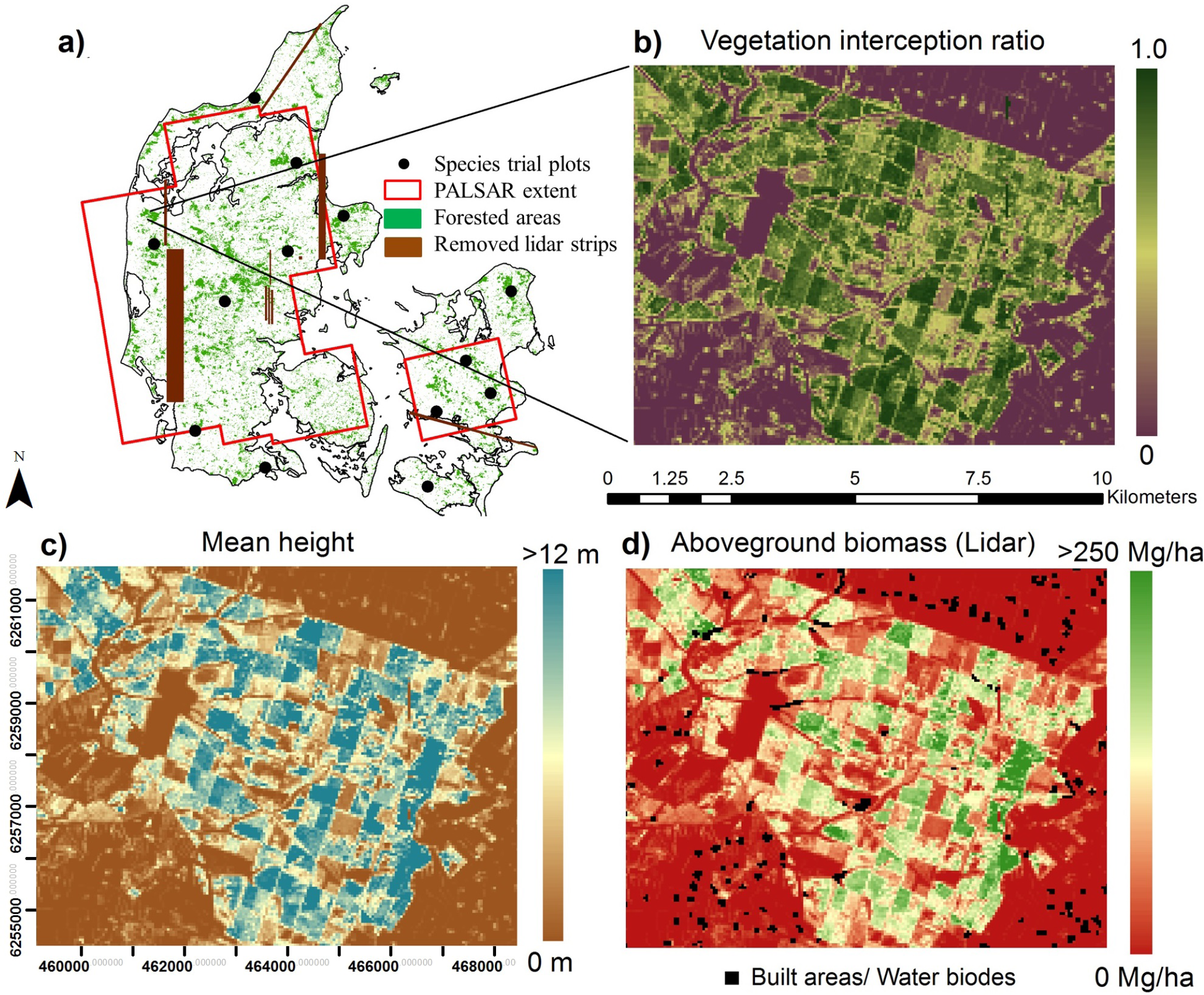
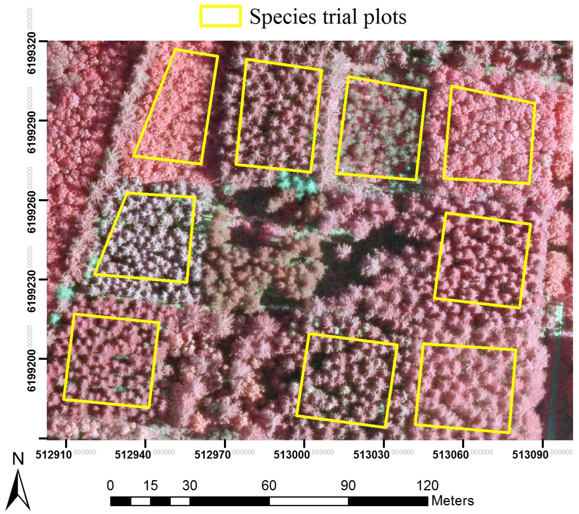
Forest tree species trial plots (STPs) were established in Denmark in the 1960s, with each containing even-aged single-species trees distributed in clusters across 13 sites (Figure 1a). Although not set up for this purpose, the design of the STPs made them well suited for investigating relations between structural forest parameters and high-resolution airborne LiDAR data. Sections of STPs were selected to reduce the influence of neighboring crowns, by placing plots within the centers of STP stands, with edges bisecting the same species and relatively similar height trees (Figure 2). The plots were inventoried in 2007/2008, with all trees cross-calipered at breast height and a subsample of 30 randomly selected trees measured for height. Biomass was estimated using wood density and expansion factors described in Skovsgaard et al. [50] and Skovsgaard and Nord-Larsen [51] in the study by Nord-Larsen and Schumacher [49]. Plot-level AGB estimates (AGB_STP), including aboveground stump, stem and branches (without foliage), were provided for this study.

Plots that were lost during stand establishment or due to catastrophic wind throws were removed for this study, resulting in a dataset of 113 plots of an area of 0.07 ha to 0.23 ha (

Table 1. Summary of the STPs (source: Johannsen et al. [46]).

Broadleaf or Conifer	Species (Latin Name)	Number of Plots	Area in Denmark (ha)
Conifer	Norway spruce (Picea abies)	11	94,728
Broadleaf	Beech (Fagus sylvatica)	11	79,376
Broadleaf	Oak (Quercus robur)	12	59,456
Conifer	Sitka spruce (Picea sitchensis)	6	36,075
Conifer	Scots pine (Pinus sylvestris)	1	35,133
Conifer	Japanese larch (Larix kaempferi)	12	23,726
Conifer	French mountain pine (Pinus mugo)	7	17,081
Conifer	Noble fir (Abies procera)	7	12,562
Conifer	Lodgepole pine (Pinus contorta)	6	12,166
Conifer	Silver fir (Abies alba)	10	11,686
Conifer	Douglas fir (Pseudotsuga menziesii)	9	6594
Conifer	Grand fir (Abies grandis)	10	5874
Conifer	Serbian spruce (Picea omorika)	1	3776
Conifer	Cypress (Chamaecyparis lawsoniana)	10	1408

). The species represented in them are the most commonly grown deciduous and conifers in Denmark [46], covering ~68% of the forest area in Denmark (conifers cover 86% of coniferous areas and broadleaves cover 49% of broadleaf areas). AGB_STP ranged 47–629 Mg ha⁻¹, similar to the range measured in the NFI across the country in 2007/2008.

2.3. Airborne LiDAR Scans

Wall-to-wall discrete-return airborne LiDAR data with an average point density of 0.5 pulses/m² (

Table 2. Summary of the airborne LiDAR and flight data collected over Denmark in spring 2006 and fall 2006/spring 2007 (source: Nord-Larsen and Schumacher [49]).

System	Optech ALTM3,100
Flying altitude	1600 m
Pulse repetition frequency	70 kHz
Scanning angle	±24°
Average point density	0.5 pulse/m2
Footprint size	50 cm
Horizontal accuracy	80 cm
Vertical accuracy	10 cm

) were collected over Denmark during leaf-off conditions in spring 2006 and fall 2006/spring 2007 by COWI. First and last return pulses were recorded and extrapolated to generate a digital elevation model (DEM) and to extract the elevation of structures above ground by the data provider. The elevation dataset has previously been shown to predict dominant tree height with a precision of ±2.5 m [52]. For this study, uncalibrated flight strips were identified upon examining the dataset and removed (Figure 1a).

2.4. ALOS PALSAR Scenes

Eleven ALOS PALSAR scenes in fine-beam dual-polarization mode (horizontal send and receive (HH) and horizontal send and vertical receive (HV)), were acquired at Level 1.5 (see Section 2.4.1) in 2007 (

Table 3. List of ALOS PALSAR scenes and acquisition dates used in the study. All scenes were taken in fine beam dual polarization mode (HH + HV) in ascending orbit.

Scene	Date	Time
ALPSRP095811100	2007/11/11	21:26:05
ALPSRP089831100	2007/10/01	21:32:49
ALPSRP089831120	2007/10/01	21:33:05
ALPSRP089831130	2007/10/01	21:33:14
ALPSRP092311100	2007/10/18	21:34:51
ALPSRP092311110	2007/10/18	21:34:59
ALPSRP092311120	2007/10/18	21:35:07
ALPSRP092311130	2007/10/18	21:35:16
ALPSRP090561100	2007/10/06	21:39:13
ALPSRP090561110	2007/10/06	21:39:22
ALPSRP090561120	2007/10/06	21:39:30

). The scenes each have an approximate dimension of 59 km in azimuth and 70 km in range, together covering ~78% of the extent of Denmark (Figure 1a). In selecting scenes, regional weather conditions for every day in the week prior to image acquisition were obtained from the Danish Meteorological Institute. Since Denmark has a typically wet climate, scenes with least precipitation around approximately the time of the airborne LiDAR scanning were sought. Pre-processing visual comparisons in areas of scene overlap, particularly over homogeneous land cover types, showed no distinguishable differences in backscatter.

2.4.1. Pre-Processing

Level 1.5 data are pre-processed for radiometric and geometric corrections after range and multi-look azimuth compression (i.e., 4 looks in azimuth and 1 in range, to a 12.5 m × 12.5 m pixel size). Terrain correcting and geo-referencing the images using a 10 m × 10 m resolution DEM (derived from a different LiDAR dataset over Denmark and available from Geodatastyrelsen) resulted in a reduction in terrain-induced distortion and geolocation errors. Georeferencing was verified by comparison to wall-to-wall, 0.16 m × 0.16 m resolution, aerial photography (available at COWI). Features, such as hedges of farms, small forest patches and islands, were found to be accurately geolocated to the sub-pixel level on the corrected images. The processing was done using the software, ASF MapReady 3.1.22 (Alaska Satellite Facility, USA).

Normalized backscatter for both polarizations ( ${\sigma }_{HH}^0$ and ${\sigma }_{HV}^0$) in the power domain (m²/m²) was mapped at a 12.5-m pixel size. Preliminary analysis showed that ${\sigma }_{HV}^0$ had a stronger relation to AGB than ${\sigma }_{HH}^0$ (Supplementary Material, Figure S1), similar to the results of previous studies covering a variety of forest ecosystems, e.g., [31,38–40,53,54]. As vegetation tends to depolarize the radar signal [24], it was relevant to focus this study on AGB, vegetation cover and ${\sigma }_{HV}^0$ relations.

2.4.2. Speckle Filtering

All SAR images have random speckle, which may mask the relationship between received backscatter signals and relevant surface interactions. Speckle must therefore be reduced before quantitative analysis, either by speckle filtering or extensive multi-looking, the latter dramatically reducing image resolution. To avoid coarsening resolution (since relations of SAR and biophysical vegetation parameters at multiple resolutions are investigated in this study), different spatial speckle reduction methods (e.g., median, Lee-sigma, local-region and Frost) and window sizes (e.g., 3 × 3, 5 × 5, 7 × 7 pixels) were tested. The aim was forest edge sharpness preservation, texture preservation and computational efficiency over the large study area. A comparison of filtered images over plantations showed that the enhanced Lee filter [55] at a 5 × 5 pixel window was most suited, as it retained stand edges, yet significantly reduced the standard deviation of ${\sigma }_{HV}^0$ over individual plantations (Supplementary Material, Figure S2). Upon coarsening map resolutions (Section 2.5.2 and Section 2.5.3), there was a further reduction in speckle, particularly at hectare scales and larger.

2.5. Model Development

2.5.1. LiDAR-to-AGB_STP Model

Point cloud elevation data from each STP were used to build a LiDAR-to-AGB_STP model. We derived variables, including the mean, maximum and minimum pulse height above ground; relative mean first pulse height (relative to maximum pulse height); variance, standard deviation, skewness, kurtosis and coefficient of variation of heights; interception ratio by canopy; and height distribution percentiles (ranging from the 25th, 50th, 75th, 95th to 99th percentile) for each STP. Most LiDAR metrics describing canopy elevation (height percentiles; maximum height; mean height; and coefficient variation of height) are highly correlated and have a similar correlation structure as vegetation biomass [56–58]. To avoid model multicollinearity, canopy height metrics showing the highest correlation with AGB_STP were selected based on the correlation matrix and cluster analysis conducted by Nord-Larsen and Schumacher [49]. However, the uncalibrated return pulse intensity used in their study showed flight-path stripes when mapped. The use of the variable would have introduced spatial bias in mapping AGB in our study, where pixel-level accuracy is required for comparing maps, and was thus avoided.

Previous studies have demonstrated that structural parameters that combine height and gap fraction improve AGB estimates from LiDAR [57,59]. A variable measuring the interception of LiDAR signals by vegetation, the vegetation interception ratio (VIR), was derived in our study. Several definitions of VIR were tested to find one that most captured differences within plantations of differing tree density and height, including the fraction of returns from various heights within plantations and the fraction of returns from the ground (Supplementary Material, Figure S3). It was found that VIR was best defined as the ratio of the number of first returns from above a 1-m height (FR_>1m) to the total number of first returns (FR) (Equation (1)).

$$\mathrm{VIR}(\text{ratio})=\frac{F{R}_{>1\mathrm{m}}}{FR}$$

(1)

Several published linear, exponential, power relations, e.g., [9,13,58,60,61], were then applied to predict AGB_STP, using forward selection of significant (p < 0.05) variables. The best LiDAR-to-AGB_STP model was selected based on the lowest Akaike information criterion (AIC) and normality of residuals. Due to the small sample size of AGB_STP, robust accuracy estimates were assessed using jackknife resampling, leaving out a random sample of 30% of data for testing in 5000 iterations. The jackknife mean relative absolute error (mRAE), mean bias error (mBias), mean root mean squared error (mRMSE) and the model coefficient of determination (R²) were used to quantify uncertainty. Dependency on plot sizes was tested by examining fit residuals after model development.

For comparison, we also attempted relating AGB_STP to ${\sigma }_{HV}^0$ using 55 STPs contained within the PALSAR extent. However, the plot areas were small compared to SAR image resolution, such that the effects of speckle were not visibly minimized on each plot, and a large number of AGB_STP values lay well above the range of SAR signal saturation. This made it impossible to map AGB with reasonable accuracy using only SAR data (Supplementary Material, Figure S4), requiring us to use the LiDAR-to-AGB_STP model to derive a country-wide AGB map.

2.5.2. SAR-to-VIR_L and SAR-to-MH_L Models

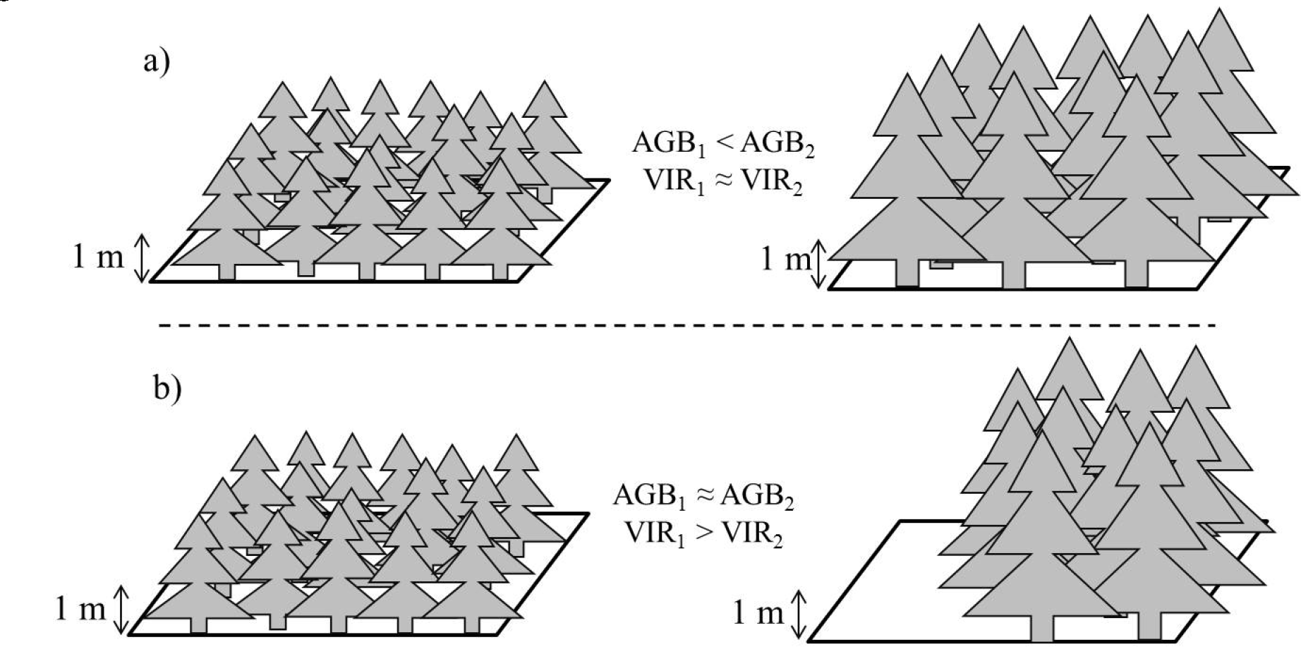
Variable VIR was first derived over the fully-forested STPs to capture vegetation penetrability (Equation (1)). On pixels with sparse vegetation or low canopy cover, the variable summarizes the heterogeneity of vegetation. Some caution must be taken in the interpretation of VIR. VIR may be positively related to, but is not, however, a direct measure of the vertical component of canopy density, since signals may be intercepted at any height above the ground >1 m. As a result, a (hypothetical) lower height, but uniformly-vegetated pixel may have the same VIR as a higher height and uniformly-vegetated pixel. Further, a lower height, but uniformly-vegetated pixel may have the same AGB density, but higher average VIR than a pixel that has only 50% tree cover, but tall and large trees (Figure 3). This variation is further complicated by differences in species types, which may have similar AGB density at a pixel scale, but varying tree distribution, stem and branch number and canopy structure. For simplicity, this study interprets VIR only as a measure of the proportion of vegetation cover (as seen by LiDAR) in each mapped pixel, independent of mean canopy height or canopy density. This portion may also be low for stands containing very young trees or low stem density. The implications of height and canopy density being related to VIR are discussed in Section 4.3.

VIR was first mapped at a 50 m × 50 m pixel size (50-m “scale”) (Figure 1b), and pixels were then averaged to coarser scales, ranging from 100 m to 500 m. SAR backscatter, ${\sigma }_{HV}^0$, at the 12.5-m scale was averaged in the power domain (m²/m²) to produce coarser scale images and regressed against average VIR both in the power and dB domain (SAR-to-VIR_L model). For comparison, ${\sigma }_{HV}^0$ was also regressed against mean canopy height (MH; SAR-to-MH_L model). At each scale, large built-up and water areas were removed entirely using a high-resolution (10 m × 10 m pixel size) land use map (available at Geodatastyrelsen). Pixels with infrastructure surrounded by agricultural lands and forested areas were removed if the infrastructure occupied ≥25% of the pixel area (e.g., Figure 1d). We verified that this threshold removed most problematic areas from the analysis and did not impact our results. For each model, the large number of pixels for calibration/validation ensures robustness without the need for jackknifing. Therefore, the dataset was randomly split into 50% training and 50% testing subsamples, which ensures confidence in the results, as the training data are independent of the testing data. All regressions were run using the CURVEFIT procedure in the software EXELIS IDL (Exelis Visual Information Solutions, Boulder, CO, USA).

2.5.3. SAR-to-AGB_L Model

The LiDAR-to-AGB_STP model was used to map AGB density across Denmark (AGB_L in units of Mg ha⁻¹) at 50-m scale first, comparable to the largest STP plot (0.23 ha), and AGB_L pixels were subsequently aggregated by averaging to coarser scales. Built-up and water areas were removed using the same procedure as in Section 2.5.2, before testing the ${\sigma }_{HV}^0$ to AGB_L relation (SAR-to-AGB_L model).

There is a large volume of studies, e.g., [11,31,37,39,53,62,63], that have developed AGB-backscatter relations through either radiative transfer models or empirical regressions [64]. The familiar loss of sensitivity of ${\sigma }_{HV}^0$ to high AGB values (typically ~100 Mg ha⁻¹ for L-band SAR) is apparent in most of these studies. Further, backscatter is often interpreted as a function of biomass, and ${\sigma }_{HV}^0$ is thus usually used as a response variable. While it is interesting to analyze the effect of using different models on our data, it is not relevant to the aims of this study. Instead, we focus on finding a single, statistically robust fit that can describe the backscatter-biomass relation best for the datasets. The fit with a balance between the least bias, least root mean squared error (RMSE) and well-distributed residuals was chosen as the best-fit model, using 50% of the dataset for training and 50% for testing. A sensitivity analysis to errors in AGB_L (mRMSE and mBias obtained through the jackknife resampling, Section 2.5.1) was conducted using simulations discussed in Section 3.2.4. We assumed throughout that the model error is additive, i.e., the random error on the model fit does not increase as variable values increase.

Although we focus on ${\sigma }_{HV}^0$ relations to vegetation cover in this study, we tested whether models, including both ${\sigma }_{HV}^0$ and ${\sigma }_{HH}^0$, e.g., [11,65], provided lower RMSE during AGB_L prediction than those using ${\sigma }_{HV}^0$ alone. We further tested whether ${\sigma }_{HH}^0$ had any relation to residuals of our selected model, to assess its ability to improve AGB_L prediction.

3. Results

3.1. Predicting AGB_STP with LiDAR

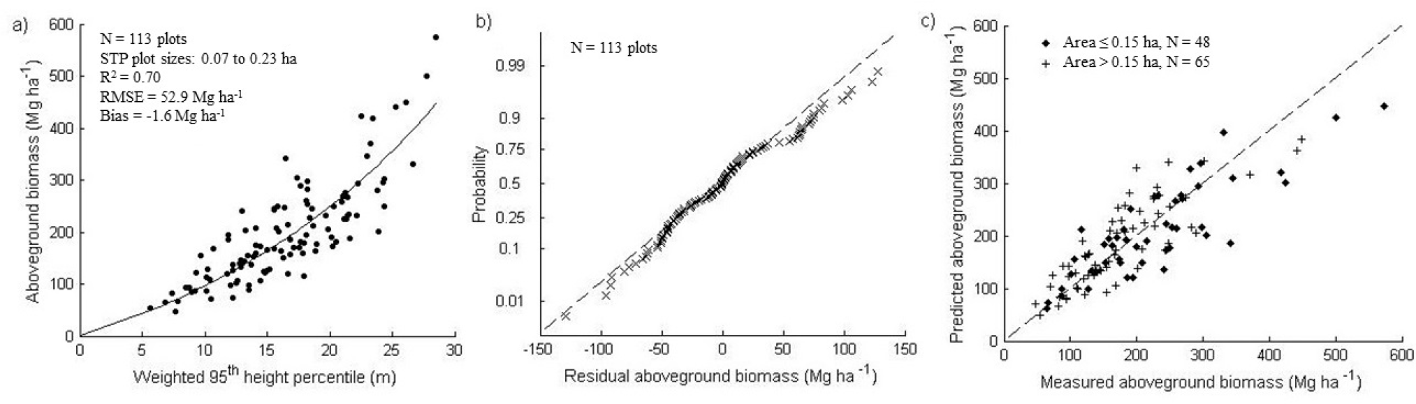
There was a strong relation between most LiDAR metrics and AGB_STP, modeled using exponential or power functions. The regression with the lowest AIC was an exponential function, including two predictor variables: the 95th percentile of canopy height from returns above 1 m (P₉₅), multiplied by VIR, explaining 70% of the variation in AGB_STP (Figure 4a,

Table 4. Summary of the results of the LiDAR-to-AGB_STP model (Equation (2)).

LiDAR-to-AGBSTP Model
Parameter	Estimate	Standard Error	t-Stat	p-value
a	166.18	44.02	3.78	0.0003
b	0.05	0.01	5.84	0.0000
R2	0.70	–	–	–
RMSE (Mg ha−1)	52.9	–	–	–
Bias (Mg ha−1)	−1.6	–	–	–

).

$${\mathrm{AGB}}_{\mathrm{STP}}(\mathrm{Mg}{\mathrm{ha}}^{-1})=a({\mathrm{e}}^{(b\mathrm{VIR}.{\mathrm{P}}_{95})}-1)$$

(2)

Fit residuals were normally distributed (Shapiro–Wilk test of normality with p = 0.17) with low systematic under-prediction of high AGB (Figure 4b). Further, there was no dependence of residual distribution on STP plot size (Figure 4c). Validation statistics showed that AGB_STP is retrieved with mRMSE of 53.8 Mg ha⁻¹ and mBias of −2.0 Mg ha⁻¹ (

Table 5. Summary of the LiDAR-to-AGB_STP model validation using jackknife resampling. R_i and P_i are the ground-measured and model-predicted values for sample i, respectively, and n is the number of samples.

LiDAR-to-AGBSTP Model Validation
Metric	Equation	Validation Statistic	Standard Deviation
mRMSE (Mg ha−1)	$\sqrt{\frac{1}{n}{{\displaystyle \sum _{i=1}^n(P_i-R_i)}}^2}$	53.8	6.4
mRAE (%)	$\frac{1}{n}{\displaystyle \sum _{i=1}^n\frac{|P_i-R_i|}{R_i}}\times 100\%$	21.8	–
mBias (Mg ha−1)	$\frac{1}{n}{\displaystyle \sum _{i=1}^n(P_i-R_i)}$	−2.0	11.6

).

3.2. Multi-Scale SAR Relations to Vegetation Cover, Height and AGB_L

The following sections detail relations between SAR backscatter and LiDAR-derived vegetation descriptors for the whole study area. Results from only a few spatial scales are reported to demonstrate the observed trends.

3.2.1. Up-Scaling and Forest Edges

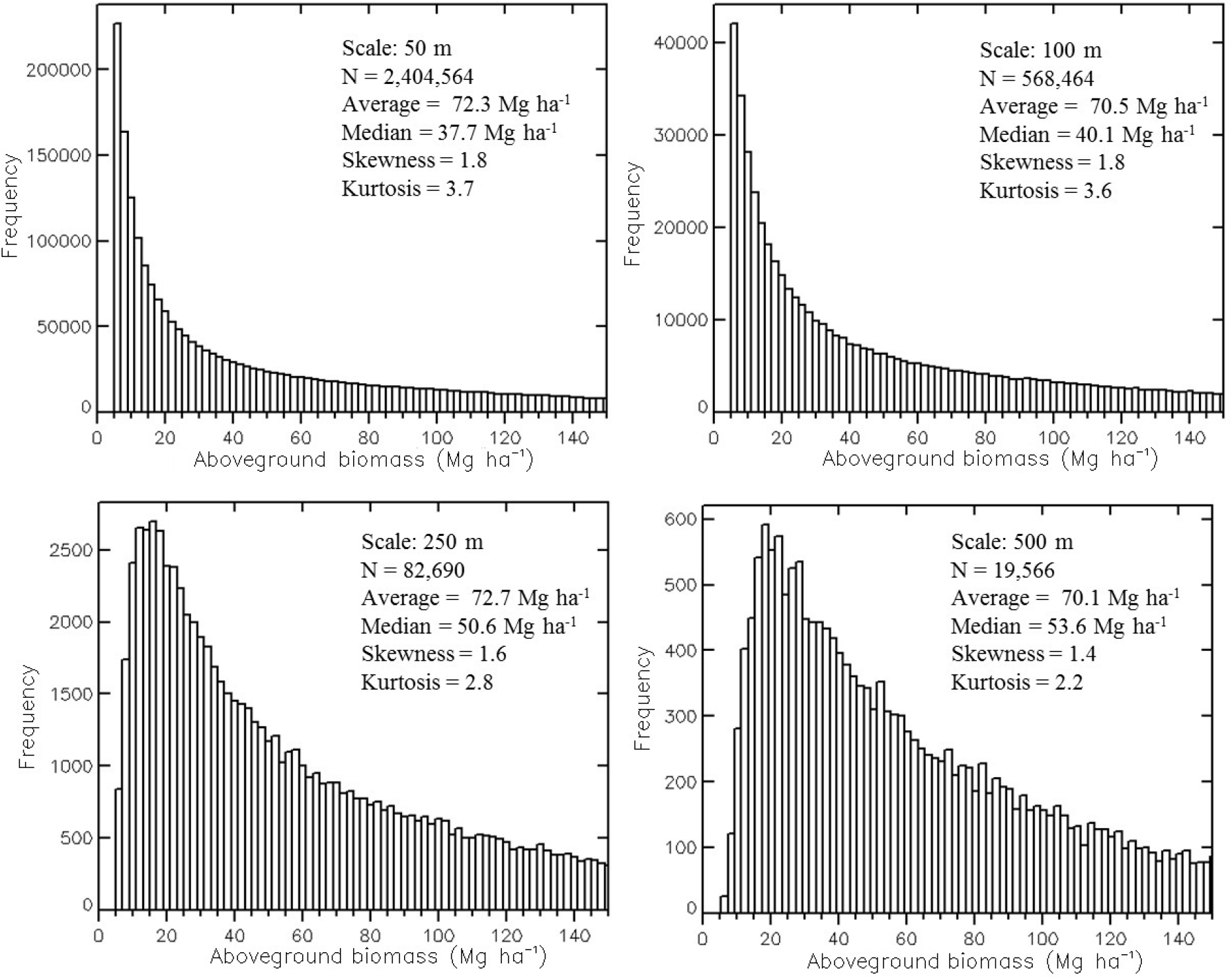
In aggregating pixels from fine to coarse scales, consideration must be given to forest edges, which are lost by averaging over them. The inclusion or exclusion of edge pixels was found to influence model performance and retrieval accuracy. Thus, a number of methods were tested to fairly represent only forested areas and pixels along forest edges, as scales are coarsened from 50 m on, before any quantitative analysis. First, areas with AGB ≤ 5 Mg ha⁻¹ were flagged and removed from the maps at 50-m scale. Further, some agricultural lands were identified with high VIR (>0.7) and low mean and maximum height (<1.5 m) and removed. These thresholds allowed a large portion of bare-ground or agricultural fields to be removed, i.e., ~89% of pixels classified as ‘potentially agriculture’ in the Danish land use map (Geodatastyrelsen) discarded as a result. The remaining pixels identified as ‘potentially agriculture’ were found to be: (1) vegetated hedgerows; (2) forest-edges; and (3) areas of young forest plantations, divisions between individual plantations and, in some cases, harvested forests. These were retained for analysis at 50-m scale. For each coarser scale map, pixels were only included if they had AGB >5 Mg ha⁻¹ and if less than a certain threshold of discarded pixels at 50 m were contained with them (Supplementary Material, Figure S5). This threshold was selected such that the average AGB represented across the landscape at each spatial scale remains nearly constant (Figure 5). Hence, primarily vegetated pixels are being examined at each scale and nearly the same forest stands being compared across scales, with the loss of comparatively small forest patches as scales coarsen. Once this was done, there was no significant influence of remaining forest-edge pixels on the general trends in SAR relations to LiDAR variables when comparing results across scales.

3.2.2. SAR-to-VIR_L Model

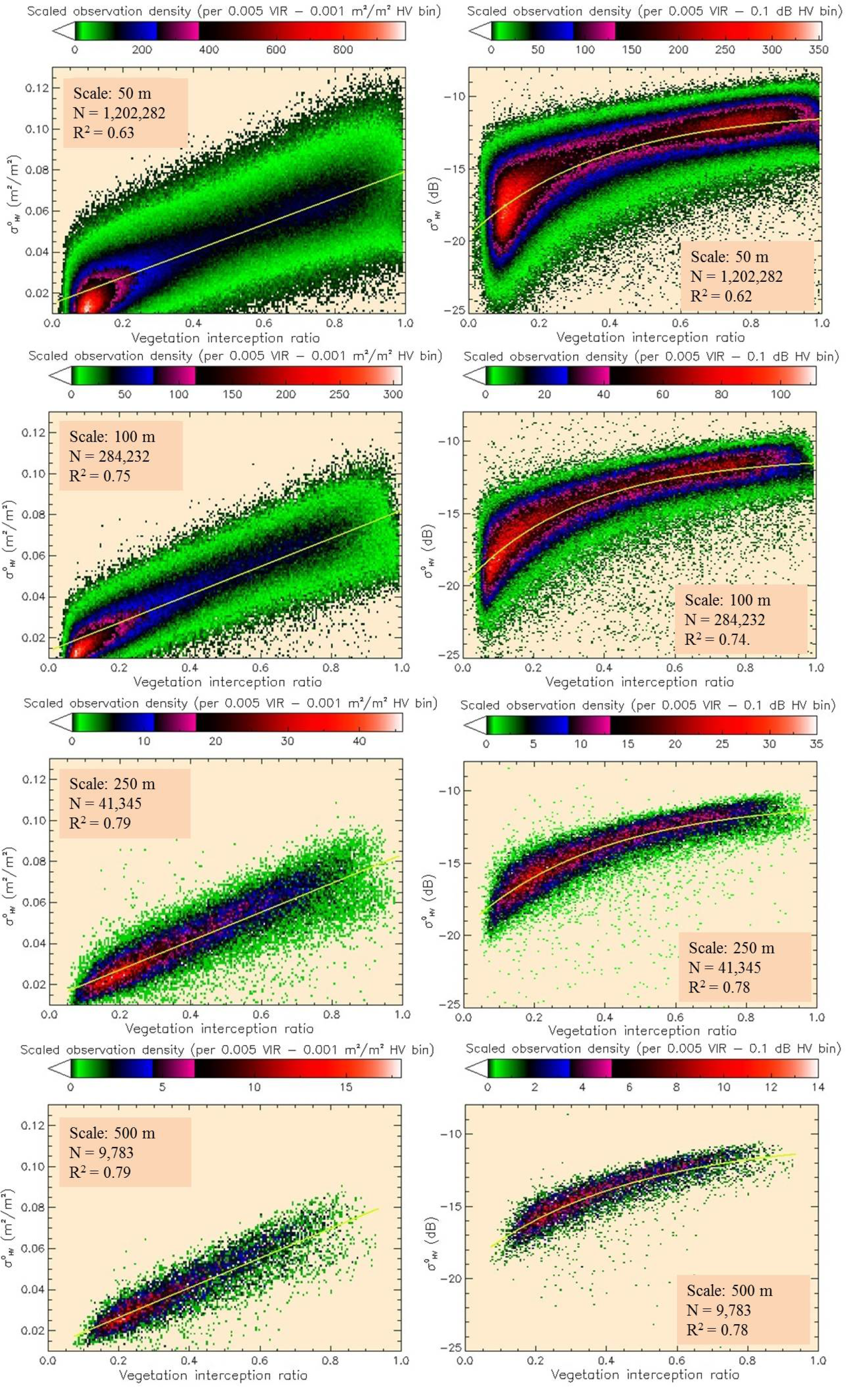
Backscatter in the power domain (m²/m²) was found to have a positive linear relation to average VIR (Figure 6, left).

$${\sigma }_{HV}^0(m^2/m^2)=d\mathrm{VIR}+g$$

(3)

The scatter in the data is relatively weakly explained at 50-m scale (R² = 0.63) and improves at coarser scales (up to R² = 0.79 at ≥ 250 m) (

Table 6. Results of SAR-to-VIR_L model for the validation dataset. d and g are regression coefficients used in Equation (3), reported with the standard error. The last two columns show regression results when building the model with ${\sigma }_{HV}^0$ in dB. Significance is provided as * p-value < 0.01.

SAR-to-VIRL
Scale	R2	RMSE	Bias	d	g	R2 (dB model)	RMSE (dB model)
m		m2/m2	m2/m2				dB
50	0.63	0.014	< 10−5	0.065 ± 0.000*	0.015 ± 0.000*	0.62	1.72
100	0.75	0.011	< 10−5	0.070 ± 0.000*	0.013 ± 0.000*	0.74	1.29
250	0.79	0.008	< 10−5	0.072 ± 0.000*	0.013 ± 0.000*	0.78	0.87
500	0.79	0.007	< 10−5	0.073 ± 0.000*	0.012 ± 0.000*	0.78	0.81

).

As there is no apparent loss of sensitivity of ${\sigma }_{HV}^0$ to high VIR values, it was reasonable to build the model in the power domain, making it possible to distinguish high ${\sigma }_{HV}^0$ at intervals comparable to low ${\sigma }_{HV}^0$ values. However, since this trend is not expected in the SAR-to-MH_L and SAR-to-AGB_L models (due to signal saturation), we also tested and report SAR-to-VIR_L performance in the dB domain (Figure 6, right) using the best-fitted exponential model $(Y={\alpha }_0{e}^{{\alpha }_{1}X}+{\alpha }_2)$. Trends across spatial scales were found to be the same, with prediction RMSE improving with coarsening scale (Table 6, model coefficients not shown).

3.2.3. SAR-to-AGB_L and SAR-to-MH_L Model

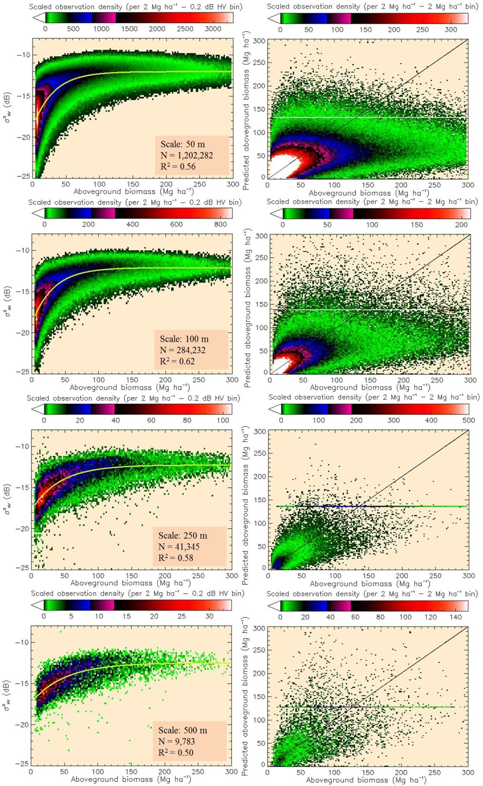
The ${\sigma }_{HV}^0$ images showed good qualitative agreement with the AGB_L map at 50-m scale, with no observable geolocation errors. The variation in ${\sigma }_{HV}^0$ across the landscape was best explained (highest R²) by an SAR-to-AGB_L model defined as:

$${\sigma }_{HV}^0(\mathrm{dB})=c+a(1-{\mathrm{e}}^{b{\mathrm{AGB}}_{\mathrm{L}}})$$

(4)

where a, b and c are constants. Although the fit is empirical, it resembles the simplified form of the water cloud model [66] used in previous studies [37,38,53,67] to relate AGB and backscatter. Here, it was chosen due to the high R² values and low RMSE values achieved (

Table 7. Results of the SAR-to-AGB_L model. a, b and c are regression coefficients used in Equation (4), reported with the standard error. Significance is provided as * p-value < 0.01.

SAR-to-AGBL Model
Scale	R2	RMSE	Bias	a	b	c
m		dB	dB
50	0.56	1.86	< 10−5	6.805 ± 0.006*	−0.032 ± 0.000*	−18.833 ± 0.006*
100	0.62	1.57	< 10−5	6.748 ± 0.011*	−0.031 ± 0.000*	−18.831 ± 0.012*
250	0.58	1.23	< 10−5	5.450 ± 0.027*	−0.022 ± 0.000*	−17.642 ± 0.030*
500	0.50	1.11	< 10−5	4.653 ± 0.061*	−0.019 ± 0.000*	−17.113 ± 0.071*

), rather than for theoretical reasons. It must be noted that the fitted model accommodates for a decrease in backscatter with increasing AGB, which may physically be caused by increasing forest opacity (as explained by the water cloud model), as well as macroecological trends in stem sizes and number density as AGB increases [68]. The strongest relations across all scales resulted from fitting Equation (4) both in dB (Figure 7) and the power domain (Supplementary Material, Figure S6). The scatter in the AGB_L-backscatter relation was best explained at 100–150-m scales (R² = 0.62) and weakened in comparison at scales ≥250 m (R² ≤ 0.58), while the RMSE improves with coarsening resolution. This difference arises since the RMSE is more sensitive to larger and extreme values due to the squaring of differences, which are averaged out with coarsening resolution, as compared to R², which represents how well the modeled curve explains the scatter in the data.

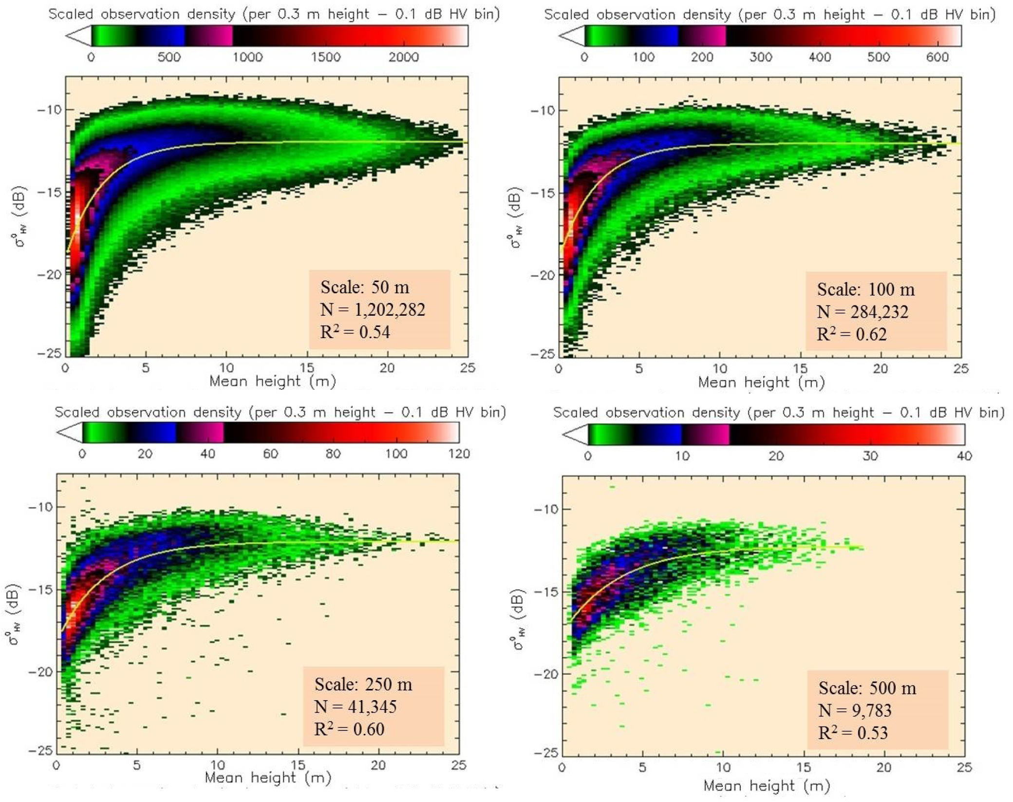
The SAR-to-MH_L model was also best developed using Equation (4). A loss of sensitivity of ${\sigma }_{HV}^0$ to canopy heights of ~7 m at 50 m (Figure 8) and a relatively weaker relation of backscatter to MH than backscatter to VIR (Supplementary Material, Figure S7, shows the SAR-to-MH_L in the power domain) were observed. The scatter in the data is comparatively better explained at fine scales (R² = 0.62 at 100 m), with some decline in the robustness of the fit at scales ≥250 m (

Table 8. Results of the SAR-to-MH_L model. a, b and c are regression coefficients used in Equation (4), reported with the standard error. Significance is provided as * p-value < 0.01.

SAR-to-MHL Model
Scale	R2	RMSE	Bias	a	b	c
m		dB	dB
50	0.54	1.89	< 10−5	7.030 ± 0.007*	−0.445 ± 0.001*	−19.011 ± 0.007*
100	0.62	1.58	< 10−5	7.042 ± 0.012*	−0.438 ± 0.002*	−19.058 ± 0.013*
250	0.60	1.20	< 10−5	5.780 ± 0.027*	−0.324 ± 0.004*	−17.830 ± 0.031*
500	0.53	1.07	< 10−5	5.071 ± 0.061*	−0.268 ± 0.0103*	−17.271 ± 0.074*

). Similar to the SAR-to-AGB_L model, the prediction RMSE improves with coarsening resolution.

Retrieving AGB from backscatter requires Equation (4) to be inverted, resulting in a logarithmic function.

$${\mathrm{AGB}}_{\mathrm{L}}(\mathrm{Mg}{\mathrm{ha}}^{-1})=\frac{1}{b}\ln (1-\frac{{\sigma }_{HV}^0-c}{a})$$

(5)

Since the inverted model is undefined for values where ${\sigma }_{HV}^0\ge c+a$ and predicts AGB < 0 Mg ha⁻¹ where ${\sigma }_{HV}^0\le c$, the inversion requires the model to be constrained to a certain range of ${\sigma }_{HV}^0$ values and a best-guess to be made where ${\sigma }_{HV}^0$ is below/above the predictable range [38]. Inverting the model to retrieve AGB results in a loss of 23%, 20%, 18% and 17% of the data where ${\sigma }_{HV}^0$ fell above the predictable range and 8%, 6%, 4% and 3% where it fell below, at scales of 50 m, 100 m, 250 m and 500 m, respectively (the number of observations, N, are reported in Figure 7). For where it fell below the predictable range, 0 Mg ha⁻¹ was considered the most reasonable best guess and assigned to predicted values.

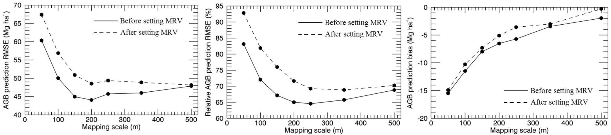
In assessing overall retrieval accuracy, two approaches were taken. First, AGB prediction RMSE and bias were derived only for values where ${\sigma }_{HV}^0$ fell below and within the predictable range. Second, a maximum retrieval value (MRV) was assigned to values where ${\sigma }_{HV}^0$ fell above the predictable range. In this method, an approach similar to that described in Santoro et al. [63] was taken and a buffer zone set to remove outliers that were most likely resultant from local environmental factors. We then tested assigning the maximum successfully predicted AGB value and increasing/decreasing the value each time by 5 Mg ha⁻¹ in multiple iterations until the minimum overall model RMSE was achieved. Furthermore, the percentile distribution of successfully predicted values was derived, and each time, a different percentile was set as the MRV until the minimum model RMSE was achieved. It should be noted that no consideration was given to bias in this method, since the overall model bias is strongly sensitive to the selected MRV, and low bias does not necessarily indicate that the best method has been chosen. Multiple test iterations showed that assigning an MRV of one of the percentile distributions of the successfully predicted data reduced the overall model RMSE most. The effect of assigning an MRV to the residual plots of predicted AGB against AGB_L is displayed in Figure 7, right.

The differences in the two approaches for multi-scale comparisons showed that the method of assigning an MRV changes absolute and relative model errors, but the trends of improving model accuracy with spatial scale remain largely similar (Figure 9). AGB retrieval accuracy and residual bias were found to improve overall with coarsening map scale. The largest improvement is observed on mapping at 100-m instead of 50-m scale, and after 250-m scale, accuracy improvement is low and even decreases with increasing scale by some metrics thereafter.

It was also found that the chosen model (Equation (4)) provided lower RMSE values in AGB prediction overall, when compared to models including both ${\sigma }_{HV}^0$ and ${\sigma }_{HH}^0$. Further, ${\sigma }_{HH}^0$ showed a negligibly weak relation to AGB residuals, suggesting that it adds no further information to AGB_L prediction than that which ${\sigma }_{HV}^0$ has already provided (Supplementary Material, Figure S8).

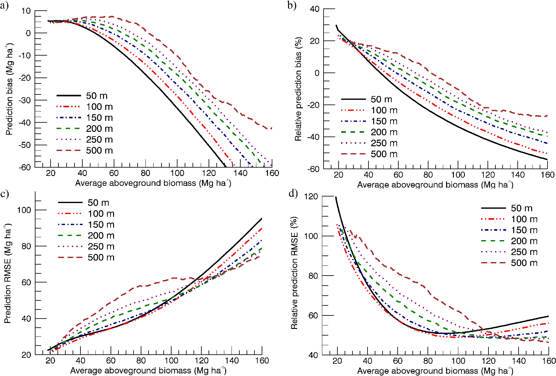
In accounting for forest edges in the multi-scale analysis (Section 3.2.1), the mean AGB of the pixels considered was nearly constant, but the distribution of measures changes as spatial variability decreases upon averaging (Figure 5). To fairly assess prediction trends across scales, we derived relative prediction bias and RMSE at each range of the independent AGB variable, which shows the degree to which the inverted model differs in accuracy for areas of different biomass ranges (Figure 10). In this analysis, we use the predicted AGB dataset before setting an MRV for the results data, to remove the stronger influence of the chosen MRV at higher AGB_L ranges compared to lower AGB_L ranges.

A continuous moving bin of 50 Mg ha⁻¹ was examined individually across the range of AGB_L. It was found that high biomass values are under-predicted by the model, particularly at fine scales, indicating a decrease of sensitivity of ${\sigma }_{HV}^0$ to AGB at an AGB value that varied with the mapping scale (Figure 10a,b). The model begins to under-predict AGB in areas with biomass >45 Mg ha⁻¹ and >80 Mg ha⁻¹ at 50-m and 500-m scale, respectively. RMSE in the bins indicated a stronger performance at 100-m scale for areas with AGB below 110 Mg ha⁻¹ and some improvement of performance when mapping at scales ≥150 m for areas with higher AGB (Figure 10c,d).

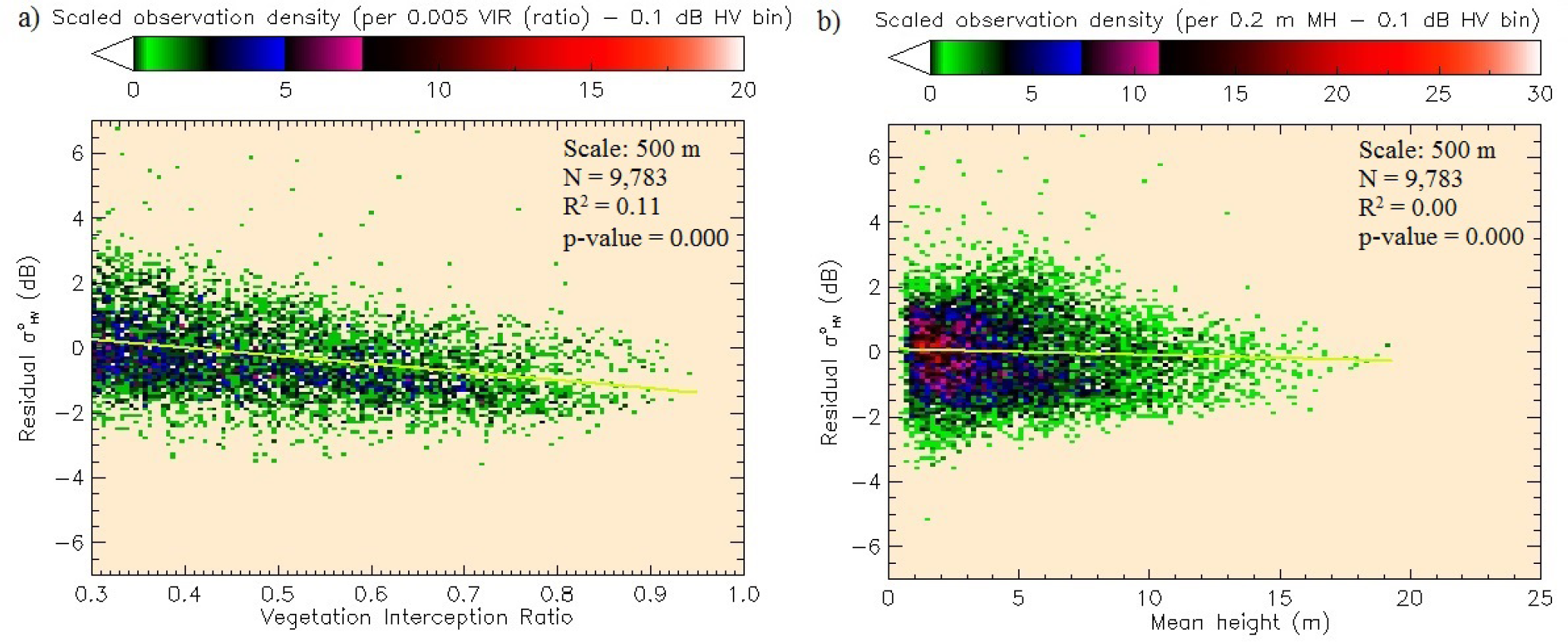
Since AGB_L was derived using VIR and P₉₅ at 50-m scale, an analysis of residual plots of the SAR-to-AGB_L model was conducted to assess whether these variables offered an explanation for the scatter in the biomass-backscatter plot. VIR showed a weak (R² = 0.11), but significant (p < 0.0001) linear relation to residual ${\sigma }_{HV}^0$ at coarse scales (≥250 m), while MH and height distribution percentiles were found to provide no additional statistical information (Figure 11a,b). It appears, therefore, that the AGB-backscatter curve is largely explained by the MH-backscatter relation, and VIR provides some additional information (i.e., 11% at 500 m) on the data scatter beyond the modeled AGB-backscatter curve. It is important to note that the analysis cannot assess whether this information can improve AGB retrieval accuracy, since AGB_L is not independent of VIR in this study.

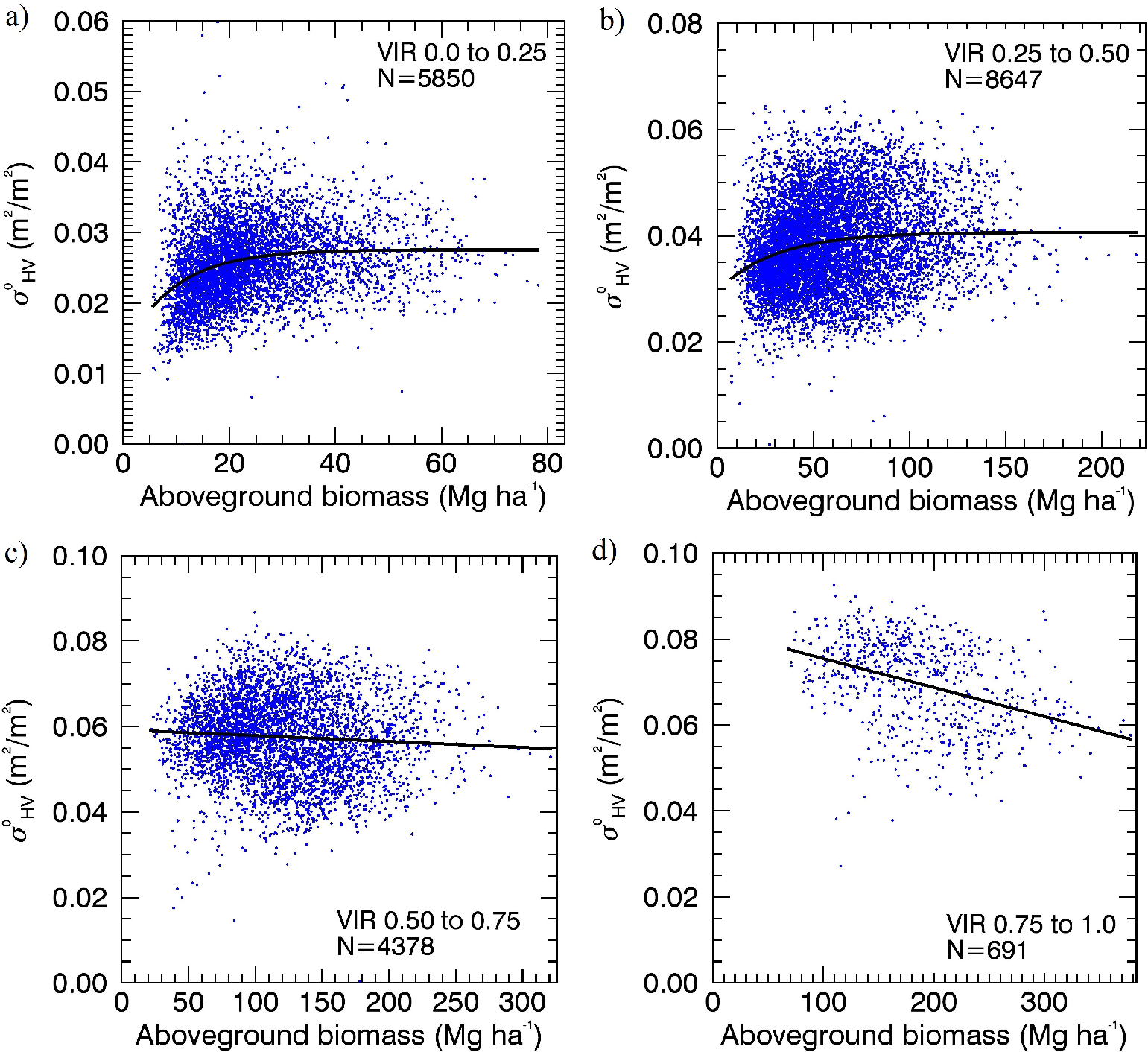
As a means of demonstration of how the fraction of forest cover can explain variations in the AGB-backscatter curve, we stratified our study area into four VIR categories (0 to 0.25, 0.25 to 0.50, 0.50 to 0.75 and 0.75 to 1.0) and re-built the SAR-to-AGB_L model on each. We allowed for the selection of both linear and asymptotic functions (e.g., Equation (4)) for the model based on R² values. We found significant differences in the shape of the biomass-backscatter curve for different VIR ranges (Figure 12). Areas of low VIR (primarily low stem density plantations and areas of low fraction of vegetation cover at VIR ≤ 0.5) were well fitted using Equation (4). In contrast, areas of high VIR (primarily fully-vegetated core plantation pixels at VIR > 0.75) showed a slight decline in ${\sigma }_{HV}^0$ as AGB_L increases. All model coefficients were significant (p < 0.0001), and ${\sigma }_{HV}^0$ is shown in the power domain (m²/m²) in Figure 12 to demonstrate the decline at high ${\sigma }_{HV}^0$ values.

3.2.4. Uncertainty Analysis in SAR-to-AGB_L

The methods of this study are primarily empirical, involving large datasets, each with inherent uncertainty. It must be specified here that the purpose of our study is to examine trends in relations and retrieval uncertainty across scales, rather than to achieve the highest possible prediction accuracy at any one scale; we do not attempt to estimate the total AGB stock of Denmark. As such, we do not integrate datasets, do not restrict our dataset to specific AGB ranges (e.g., AGB_L < 100 Mg ha⁻¹, where ${\sigma }_{HV}^0$ signal saturation may not be problematic) and assess the models’ performances by using a subset of our data for testing.

We distinguish between uncertainty related to bias and measurement errors in the original datasets. The former are only likely to cause a systematic shift in AGB_L values consistently across scales and, hence, are not relevant to multi-scale comparisons. This includes allometric-related bias in AGB_STP and systematic errors in the LiDAR data calibration. In estimating AGB_STP, all trees were cross-calipered, and hence, the sampling errors are negligible. Measurement errors in LiDAR returns used to produce AGB_L are considered negligible given the high point density of returns (Table 2) pooled together at 50-m scale.

Errors in the AGB_L map derived from the LiDAR-to-AGB_STP model (i.e., mRMSE and mBias) result in higher uncertainty in AGB retrieved from the SAR-to-AGB_L model. Two complications arise in propagating errors from one map to the other. First, the accuracy of AGB predicted by LiDAR has been previously shown to increase with coarsening resolution [19,69], but we lacked ground data to build multi-scale LiDAR-to-AGB_STP models. Since the best possible map was produced at 50-m scale and then averaged to coarser scales, we take a conservative approach and assume no reduction in AGB prediction error (mBias and mRMSE) at coarse scales. This assumption is only appropriate if systematic errors (mBias) are low at very fine scales and the residuals of the LiDAR-to-AGB_STP model are normally distributed (Figure 4b).

Second, computing uncertainty in nonlinear models with measurement errors in both the response ( ${\sigma }_{HV}^0$) and predictor (AGB_L) variables is nontrivial. There is no one method for a robust error estimation, and common substitute methods include simulation or Monte Carlo-type tests [64]. In this study, we conduct a sensitivity analysis by using different combinations of the dataset. We ran SAR-to-AGB_L models on the extremes of the values of AGB_L’s average error range (i.e., on AGB_L+mRAE% and AGB_L−mRAE%) to verify that the chosen best-fit models remained suitable for use at these ranges. Further, we simulated AGB values with an added random noise (AGB_L + N (0, mRMSE)) and ran the models on these values to derive the standard deviation of prediction bias, RMSE and R². We found that the chosen best fit remained the strongest fit at the extreme ranges AGB_L+mRAE% and AGB_L−mRAE%. Models with simulated AGB values showed an average of <0.1-Mg ha⁻¹ change in AGB retrieval accuracy, primarily due to the larger number of observations available for regression.

Finally, ${\sigma }_{HV}^0$ may vary widely between different radar scenes due to differences in acquisition dates and variations in environmental conditions across the landscape. Our SAR-to-AGB_L model was tested on each scene separately. Chosen best fits remained the same, and trends in AGB retrieval uncertainty when comparing models across different spatial scales were found to be largely similar to using the whole dataset. However, there was higher variation in scenes with a smaller proportion of land at coarser scales due to fewer data points (Supplementary Material, Figure S9). Hence, it was reasonable to use the full dataset for model training and validation, particularly for coarse scales.

4. Discussion

4.1. Biomass Retrieval Using LiDAR

Biomass retrieval models using LiDAR calibrated with data from the species trial plots showed a satisfactory level of precision for the objectives of this study, explaining 70% of the variation in AGB with an RMSE of 53.8 ± 6.4 Mg ha⁻¹. Some of the performance may be attributed to the model being trained on plots with even-aged trees, the same species composition, buffer-areas along perimeters and with forests of the same biophysical structure and management procedures. These factors can significantly reduce co-registration errors [69] and plot-edge errors [13,70] related to the use of LiDAR on small-sized plots.

Our study demonstrates the suitability of a two-step approach, in which radar images are calibrated against a higher-resolution LiDAR product, itself calibrated with ground measurements of AGB [14]. It is important to discuss the use of such an approach and the associated errors in predicting AGB across Denmark and other forest types. Since the majority of Danish forests are plantations represented by the STPs [46], we can be confident that the model performs well in these areas. The model may however not perform as well over mixed forests types, particularly by under-predicting AGB in areas with AGB >300 Mg ha⁻¹, as observed in previous studies [49]. This may result, since low-density LiDAR pulses (here, 0.5 pulses/m²) are unable to sufficiently penetrate dense canopies and extract distinguishable structural characteristics in mixed forests. Hence, replicating our study in structurally complex or high biomass forests would need higher point-density LiDAR data or models built on larger plot sizes and varied sampling designs to improve AGB retrieval accuracy [14,19,69]. Further, in averaging the LiDAR-derived AGB map (here, AGB_L) to coarser scales, we could not account for changes in model RMSE and bias due to the lack of large-area ground-data. Most studies have, however, shown marked improvements in accuracies as plot sizes increase [9,69,71,72], and hence, assuming no improvement with coarsening scale was considered a reasonable conservative approach in our study. Models built for forests with high spatial variability in vegetation structure would need to be scale-invariant [73] or need further analysis on the averaging of systematic errors with scale.

4.2. SAR Relation to Aboveground Biomass at 50 m–500 m Scales

As is common for most national, continental and global maps, our study involves building AGB-backscatter relations that cut across a complex landscape of patchy forests and agricultural lands, providing insight into AGB retrieval accuracy trends observed in areas dominated by human use. On coarsening resolution, the numerous small forest patches cause an increasing proportion of forest-edge pixels, each with high AGB variability within, but low overall AGB density. Trends across mapping scales may only be fairly compared after adequately removing these areas from the analysis (Section 3.2.1). The SAR-to-AGB_L relation examined then demonstrated that mapping scale is a critically important parameter in AGB retrieval. Retrieval accuracy improved as the pixel sizes of the SAR image and LiDAR-derived AGB map used to calibrate it (AGB_L) were increased from 50 m to 250 m, and negligibly thereafter (Figure 9). A large part of the initial improvement (50 m to 100 m) is expected from the averaging of errors inherent in radar images, such as those from speckle, thermal noise, geolocation, canopy layover and variations due to moisture or topography [11]. Improvements up to larger scales are also expected due to the reduction of local spatial variability of ${\sigma }_{HV}^0$ and AGB by averaging, reducing the bias in calibration equations used to relate these variables [14]. The negligible improvement beyond the 250-m scale indicates that there is an upper limit up to which mapping resolution needs to be coarsened before a large part of the underlying forest heterogeneity is lost and retrieval accuracy is constant. This is a relevant finding for studies that need to establish adequately-sized ground-plots to calibrate backscatter, acquired for example from the recently launched L-band ALOS PALSAR-2 mission, to AGB. Previous studies using up to 1-ha plots have noted improving AGB-backscatter relations with scale [11,74]. Our study shows that plot scales of 150–250 m (i.e., sizes of 2.25–6.25 ha) may be most suitable for mapping AGB, significantly larger than most forest inventory plots (e.g., the 707-m² area plots of the Danish NFI).

Observing results of the SAR-to-AGB_L model for regions of different biomass reveals that while AGB retrieval is more accurate at fine scales (50 m or 100 m) for areas with AGB below ~110 Mg ha⁻¹, retrieval at coarser scales is more accurate for areas with higher AGB (Figure 10d). The AGB value at which backscatter begins to lose sensitivity to AGB in the models also increases with coarsening spatial scale as the data distribution changes (Figure 10a). A comparison of model R²’s (Table 7) suggests that suitable mapping resolutions would be 100 m for low biomass areas and 250 m for high biomass areas in Denmark. These results are of relevance for studies aimed at AGB change detection using SAR, where accurate AGB estimates pre- and post-disturbances are desired [4]. Establishing a statistically optimal plot size for data calibration and an optimal biomass mapping resolution are dependent on the range of biomass considered, desired error bounds and the distribution of forests being studied across landscapes.

4.3. SAR Relation to Vegetation Height and Cover

The backscatter relation to mean vegetation height displayed similar trends of signal saturation and improvement in model accuracy with scale as the AGB-backscatter relation. This result is expected, since a height distribution percentile (P₉₅) was used to derive AGB_L, and height was thus representative of the AGB across the landscape. Mean height and other height percentiles were unable to explain any of the scatter in AGB-backscatter plot.

In contrast, relating the LiDAR-derived canopy interception ratio (VIR) to ${\sigma }_{HV}^0$ showed no saturation and a strong linear relation in the power domain. If VIR is interpreted simply as the proportion of vegetation cover in a pixel, the result shows that as more signals are scattered off of vegetation, more energy is returned to the satellite sensor. However, this interpretation alone makes no distinction between backscatter returned from forests with different canopy or stem density. Since VIR does not provide a measure of the vertical component of canopy density, some interpretation of the relation is required and discussed here. SAR signal saturation is observed even in areas of low VIR (≤ 0.5), such as low stem density plantations and areas of low fraction of vegetation cover (Figure 12). This indicates that canopy opacity may not be the only cause of signal saturation, but other factors, such as the size of scattering elements (trunks and stems) may influence saturation [43,68]. Further, a slight decreasing trend in ${\sigma }_{HV}^0$ is observed as AGB increased on forested pixels with VIR > 0.75. If increasing AGB is associated with increasing height and correspondingly larger and more numerous branches encountered in the vertical dimension, then signal attenuation may be associated with increased vertical canopy density. For long-wavelength SAR, changes in both the cross-sectional area and number density of branching elements with depth into the canopy have been theoretically shown to influence backscatter [43,45]. Our LiDAR data alone were not suitable to study the depth of the attenuating layer due to its relatively low point density. The analysis and discussion regarding VIR only provide a preliminary and demonstrative insight into the degree to which interaction with canopies explains variability in the AGB backscatter plot. To investigate how information on forest structural variables may improve AGB retrieval, however, requires mapping AGB independent of VIR and adding species-specific structural information to the models.

5. Summary and Conclusion

In this study, we have provided a characterization of the relations between cross-polarized ALOS PALSAR backscatter and LiDAR-derived vegetation cover, height and aboveground biomass at multiple map resolutions over Denmark. The study uses unique stepping-stone datasets, including a high-resolution DEM, ground-measured plots over even-aged plantations, country-wide airborne LiDAR, aerial photography and land use maps to develop these relations through empirical models. Our key results show that in complex landscapes dominated by patchy forests and human use, optimal scales to retrieve and map AGB from SAR are approximately 100 m for areas with low (< 110 Mg ha⁻¹) and 250 m for areas with high AGB. Improvement in retrieval at scales coarser than 250 m is negligible. Furthermore, backscatter loses sensitivity to height and biomass where these variables are relatively high, but showed a linear relation to a metric measuring the fraction of vegetation cover at >1 m height and LiDAR signal penetrability (VIR). VIR explained some of the observed scatter in the biomass-backscatter relation at very coarse scales (≥ 250 m), such that in areas of high VIR (≥0.75), there is a slight decline in backscatter as biomass increased.

Broadly, our study reinforces that spatial scale and vegetation structural properties are essential to consider when using SAR backscatter as an indicator of biomass. Particularly, for large-scale national or continental maps that cut across heterogeneous or dense vegetation types, information on the distribution of forest cover and structure will support accurate AGB retrieval. Airborne or spaceborne LiDAR surveys can readily provide such information, and future products from ICESat-2, GEDI and MOLI will hence be an important data source for AGB mapping. Further examination of the relationships explored in the study is also certain to provide a stronger basis for designing protocols to map vegetation biomass using radar data from ALOS PALSAR-2 and the future BIOMASS mission.

remotesensing-07-04442-s001.pdf

References

- Gibbs, H.K.; Brown, S.; Niles, J.O.; Foley, J.A. Monitoring and estimating tropical forest carbon stocks: Making REDD a reality. Environ. Res. Lett. 2007, 2, 045023. [Google Scholar]
- Pan, Y.; Birdsey, R.A.; Fang, J.; Houghton, R.; Kauppi, P.E.; Kurz, W.A.; Phillips, O.L.; Shvidenko, A.; Lewis, S.L.; Canadell, J.G.; et al. A large and persistent carbon sink in the world’s forests. Science 2011, 333, 988–993. [Google Scholar]
- UNFCCC, United Nations Framework Convention on Climate Change. Fact sheet: Reducing emissions from deforestation in developing countries: Approaches to stimulate action; 2011.
- Houghton, R.A.; Hall, F.; Goetz, S.J. Importance of biomass in the global carbon cycle. J. Geophys. Res.: Biogeosci. 2009, 114. [Google Scholar] [CrossRef]
- Hall, F.; Saatchi, S.; Dubayah, R. PREFACE: DESDynI VEG-3D Special Issue. Remote Sens. Environ. 2011, 115, 2752. [Google Scholar]
- Houghton, R.A.; Lawrence, K.T.; Hackler, J.L.; Brown, S. The spatial distribution of forest biomass in the Brazilian Amazon: A comparison of estimates. Glob. Chang. Biol. 2001, 7, 731–746. [Google Scholar]
- Mitchard, E.T.; Saatchi, S.S.; Baccini, A.; Asner, G.P.; Goetz, S.J.; Harris, N.L.; Brown, S. Uncertainty in the spatial distribution of tropical forest biomass: A comparison of pan-tropical maps. Carbon Balance Manag. 2013, 8, 1–13. [Google Scholar]
- Mitchard, E.T.A.; Feldpausch, T.R.; Brienen, R.J.W.; Lopez-Gonzalez, G.; Monteagudo, A.; Baker, T.R.; Lewis, S.L.; Lloyd, J.; Quesada, C.A.; Gloor, M.; et al. Markedly divergent estimates of Amazon forest carbon density from ground plots and satellites. Glob. Ecol. Biogeogr. 2014, 23, 935–946. [Google Scholar]
- Asner, G.P.; Powell, G.V.N.; Mascaro, J.; Knapp, D.E.; Clark, J.K.; Jacobson, J.; Kennedy-Bowgoin, T.; Balaji, A.; Paez-Acosta, G.; Victoria, E.; et al. High-resolution forest carbon stocks and emissions in the Amazon. Proc. Natl. Acad. Sci. USA 2010, 107, 16738–16742. [Google Scholar]
- Baccini, A.; Goetz, S.J.; Walker, W.S.; Laporte, N.T.; Sun, M.; Sulla-Menashe, D.; Hackler, J.; Beck, P.S.A.; Dubayah, R.; Friedl, M.A.; et al. Estimated carbon dioxide emissions from tropical deforestation improved by carbon-density maps. Nat. Clim. Chang. 2012, 2, 182–185. [Google Scholar]
- Saatchi, S.S.; Marlier, M.; Chazdon, R.L.; Clark, D.B.; Russell, A.E. Impact of spatial variability of tropical forest structure on radar estimation of aboveground biomass. Remote Sens. Environ. 2011, 115, 2836–2849. [Google Scholar]
- Montesano, P.; Cook, B.; Sun, G.; Simard, M.; Nelson, R.; Ranson, K.; Zhang, Z.; Luthcke, S. Achieving accuracy requirements for forest biomass mapping: A spaceborne data fusion method for estimating forest biomass and LiDAR sampling error. Remote Sens. Environ. 2013, 130, 153–170. [Google Scholar]
- Mascaro, J.; Detto, M.; Asner, G.P.; Muller-Landau, H.C. Evaluating uncertainty in mapping forest carbon with airborne LiDAR. Remote Sens. Environ. 2011, 115, 3770–3774. [Google Scholar]
- Réjou-Méchain, M.; Muller-Landau, H.C.; Detto, M.; Thomas, S.C.; Le Toan, T.; Saatchi, S.S.; Barreto-Silva, J.S.; Bourg, N.A.; Bunyavejchewin, S.; Butt, N.; et al. Local spatial structure of forest biomass and its consequences for remote sensing of carbon stocks. Biogeosci. Discuss. 2014, 11, 5711–5742. [Google Scholar]
- Sinha, S.; Jeganathan, C.; Sharma, L.; Nathawat, M. A review of radar remote sensing for biomass estimation. Int. J. Environ. Sci. Technol. 2015, 12, 1779–1792. [Google Scholar]
- Asner, G.P. Tropical forest carbon assessment: Integrating satellite and airborne mapping approaches. Environ. Res. Lett. 2009, 4, 034009. [Google Scholar]
- Goetz, S.J.; Baccini, A.; Laporte, N.T.; Johns, T.; Walker, W.; Kellndorfer, J.; Houghton, R.A.; Sun, M. Mapping and monitoring carbon stocks with satellite observations: A comparison of methods. Carbon Balance Manag. 2009, 4. [Google Scholar] [CrossRef]
- Lefsky, M.A.; Cohen, W.B.; Parker, G.G.; Harding, D.J. LiDAR Remote Sensing for Ecosystem Studies. BioScience 2002, 52, 19–30. [Google Scholar]
- Zolkos, S.; Goetz, S.; Dubayah, R. A meta-analysis of terrestrial aboveground biomass estimation using LiDAR remote sensing. Remote Sens. Environ. 2013, 128, 289–298. [Google Scholar]
- Goetz, S.J.; Dubayah, R.O. Advances in remote sensing technology and implications for measuring and monitoring forest carbon stocks and change. Carbon Balance Manag. 2013, 2, 231–244. [Google Scholar]
- Angelsen, A. Moving Ahead with REDD: Issues, Options and Implications; Center for International Forestry Research: Bogor, Indonesia, 2008. [Google Scholar]
- Mascaro, J.; Asner, G.; Davies, S.; Dehgan, A.; Saatchi, S. These are the days of lasers in the jungle. Carbon Balance Manag. 2014, 9, 1–3. [Google Scholar]
- Singh, U.; Keckhut, P.; Valinia, A. First International Workshop on Space-Based LiDAR Remote Sensing Techniques and Emerging Technologies [Conference Reports]. IEEE Geosci. Remote Sens. Mag. 2014, 2, 91–93. [Google Scholar]
- Woodhouse, I. Introduction to Microwave Remote Sensing; CRC Press Taylor & Francis Group: Boca Raton, FL, USA, 2006. [Google Scholar]
- Lucas, R.M.; Mitchell, A.L.; Rosenqvist, A.; Proisy, C.; Melius, A.; Ticehurst, C. The potential of L-band SAR for quantifying mangrove characteristics and change: Case studies from the tropics. Aquat. Conserv. Mar. Freshw. Ecosyst. 2007, 17, 245–264. [Google Scholar]
- Mermoz, S.; Toan, T.L.; Villard, L.; Réjou-Méchain, M.; Seifert-Granzin, J. Biomass assessment in the Cameroon savanna using ALOS PALSAR data. Remote Sens. Environ. 2014, 155, 109–119. [Google Scholar]
- Rignot, E.; Way, J.; Williams, C.; Viereck, L. Radar estimates of aboveground biomass in boreal forests of interior Alaska. IEEE Trans. Geosci. Remote Sens. 1994, 32, 1117–1124. [Google Scholar]
- Watanabe, M.; Shimada, M.; Rosenqvist, A.; Tadono, T.; Matsuoka, M.; Romshoo, S.A.; Ohta, K.; Furuta, R.; Nakamura, K.; Moriyama, T. Forest Structure Dependency of the Relation Between L-Band σ0 and Biophysical Parameters. IEEE Trans. Geosci. Remote Sens. 2006, 44, 3154–3165. [Google Scholar]
- Sandberg, G.; Ulander, L.; Fransson, J.; Holmgren, J.; Toan, T.L. L- and P-band backscatter intensity for biomass retrieval in hemiboreal forest. Remote Sens. Environ. 2011, 115, 2874–2886. [Google Scholar]
- Cartus, O.; Santoro, M.; Kellndorfer, J. Mapping forest aboveground biomass in the Northeastern United States with ALOS PALSAR dual-polarization L-band. Remote Sens. Environ. 2012, 124, 466–478. [Google Scholar]
- Mitchard, E.T.A.; Saatchi, S.S.; Woodhouse, I.H.; Nangendo, G.; Ribeiro, N.S.; Williams, M.; Ryan, C.M.; Lewis, S.L.; Feldpausch, T.R.; Meir, P. Using satellite radar backscatter to predict above-ground woody biomass: A consistent relationship across four different African landscapes. Geophys. Res. Lett. 2009, 36. [Google Scholar] [CrossRef]
- Dobson, M.; Ulaby, F.; LeToan, T.; Beaudoin, A.; Kasischke, E.; Christensen, N. Dependence of radar backscatter on coniferous forest biomass. IEEE Trans. Geosci. Remote Sens. 1992, 30, 412–415. [Google Scholar]
- Imhoff, M.L. A theoretical analysis of the effect of forest structure on synthetic aperture radar backscatter and the remote sensing of biomass. IEEE Trans. Geosci. Remote Sens. 1995, 33, 341–352. [Google Scholar]
- Le Toan, T.; Beaudoin, A.; Riom, J.; Guyon, D. Relating forest biomass to SAR data. IEEE Trans. Geosci. Remote Sens. 1992, 30, 403–411. [Google Scholar]
- Lucas, R.M.; Cronin, N.; Lee, A.; Moghaddam, M.; Witte, C.; Tickle, P. Empirical relationships between AIRSAR backscatter and LiDAR-derived forest biomass, Queensland, Australia. Remote Sens. Environ. 2006, 100, 407–425. [Google Scholar]
- Imhoff, M.L. Radar backscatter and biomass saturation: Ramifications for global biomass inventory. IEEE Trans. Geosci. Remote Sens. 1995, 33, 511–518. [Google Scholar]
- Luckman, A.; Baker, J.; HonzÃąk, M.; Lucas, R. Tropical forest biomass density estimation using JERS-1 SAR: Seasonal variation, confidence limits, and application to image mosaics. Remote Sens. Environ. 1998, 63, 126–139. [Google Scholar]
- Peregon, A.; Yamagata, Y. The use of ALOS/PALSAR backscatter to estimate above-ground forest biomass: A case study in Western Siberia. Remote Sens. Environ. 2013, 137, 139–146. [Google Scholar]
- Englhart, S.; Keuck, V.; Siegert, F. Aboveground biomass retrieval in tropical forests—The potential of combined X- and L-band SAR data use. Remote Sens. Environ. 2011, 115, 1260–1271. [Google Scholar]
- Suzuki, R.; Kim, Y.; Ishii, R. Sensitivity of the backscatter intensity of ALOS/PALSAR to the above-ground biomass and other biophysical parameters of boreal forest in Alaska. Polar Sci. 2013, 7, 100–112. [Google Scholar]
- Patenaude, G.; Milne, R.; Dawson, T.P. Synthesis of remote sensing approaches for forest carbon estimation: Reporting to the Kyoto Protocol. Environ. Sci. Policy. 2005, 8, 161–178. [Google Scholar]
- Woodhouse, I.H.; Mitchard, E.T.A.; Brolly, M.; Maniatis, D.; Ryan, C.M. Radar backscatter is not a ‘direct measure’ of forest biomass. Nat. Clim. Chang. 2012, 2, 556–557. [Google Scholar]
- Woodhouse, I. Predicting backscatter-biomass and height-biomass trends using a macroecology model. IEEE Trans. Geosci. Remote Sens. 2006, 44, 871–877. [Google Scholar]
- Smith-Jonforsen, G.; Folkesson, K.; Hallberg, B.; Ulander, L.M.H. Effects of forest biomass and stand consolidation on P-Band backscatter. IEEE Geosci. Remote Sens. Lett. 2007, 4, 669–673. [Google Scholar]
- Brolly, M.; Woodhouse, I.H. Vertical backscatter profile of forests predicted by a macroecological plant model. Int. J. Remote Sens. 2013, 34, 1026–1040. [Google Scholar]
- Johannsen, V.K.; Nord-Larsen, T.; Riis-Nielsen, T.; Suadicani, K.; Jørgensen, B.B. Skove og plantager; Skov and Landskab: Frederiksberg, Denmark, 2012; chapter Skovressourcer. [Google Scholar]
- Nielsen, O.K.; Plejdrup, M.S.; Winther, M.; Nielsen, M.; Gyldenkærne, S.; Mikkelsen, M.H.; Albrektsen, R.; Thomsen, M.; Hjelgaard, K.; mann, L.H.; et al. Denmark’s National Inventory Report 2013; Emission Inventories 1990–2011—Submitted under the United Nations Framework Convention on Climate Change and the Kyoto Protocol; Aarhus University, DCE-Danish Centre for Environment and Energy: Aarhus, Denmark, 2013; p. 1202. [Google Scholar]
- Nielsen, O.K.; Plejdrup, M.S.; Winther, M.; Nielsen, M.; Gyldenkærne, S.; Mikkelsen, M.H.; Albrektsen, R.; Thomsen, M.; Hjelgaard, K.; mann, L.H.; et al. Denmark’s National Inventory Report 2014; Emission Inventories 1990–2011—Submitted under the United Nations Framework Convention on Climate Change and the Kyoto Protocol; Aarhus University, DCE-Danish Centre for Environment and Energy: Aarhus, Denmark, 2014; p. 1214. [Google Scholar]
- Nord-Larsen, T.; Schumacher, J. Estimation of forest resources from a country wide laser scanning survey and national forest inventory data. Remote Sens. Environ. 2012, 119, 148–157. [Google Scholar]
- Skovsgaard, J.P.; Bald, C.; Nord-Larsen, T. Functions for biomass and basic density of stem, crown and root system of Norway spruce (Picea abies (L.) Karst.) in Denmark. Scan. J. For. Res. 2011, 26, 3–20. [Google Scholar]
- Skovsgaard, J.; Nord-Larsen, T. Biomass, basic density and biomass expansion factor functions for European beech (Fagus sylvatica L.) in Denmark. Eur. J. For. Res. 2012, 131, 1035–1053. [Google Scholar]
- Nord-Larsen, T.; Riis-Nielsen, T. Developing an airborne laser scanning dominant height model from a countrywide scanning survey and national forest inventory data. Scan. J. For. Res. 2010, 25, 262–272. [Google Scholar]
- Mitchard, E.T.A.; Saatchi, S.S.; White, L.J.T.; Abernethy, K.A.; Jeffery, K.J.; Lewis, S.L.; Collins, M.; Lefsky, M.A.; Leal, M.E.; Woodhouse, I.H.; Meir, P. Mapping tropical forest biomass with radar and spaceborne LiDAR in Lopé National Park, Gabon: Overcoming problems of high biomass and persistent cloud. Biogeosciences 2012, 9, 179–191. [Google Scholar]
- Hamdan, O.; Aziz, H.K.; Hasmadi, I.M. L-band ALOS PALSAR for biomass estimation of Matang Mangroves, Malaysia. Remote Sens. Environ. 2014, 155, 69–78. [Google Scholar]
- Lopes, A.; Touzi, R.; Nezry, E. Adaptive speckle filters and scene heterogeneity. IEEE Trans. Geosci. Remote Sens. 1990, 28, 992–1000. [Google Scholar]
- Lefsky, M.A.; Hudak, A.T.; Cohen, W.B.; Acker, S. Patterns of covariance between forest stand and canopy structure in the Pacific Northwest. Remote Sens. Environ. 2005, 95, 517–531. [Google Scholar]
- Li, Y.; Andersen, H.E.; McGaughey, R. A comparison of statistical methods for estimating forest biomass from light detection and ranging data. West. J. Appl. For. 2008, 23, 223–231. [Google Scholar]
- Næsset, E.; Bollandsås, O.M.; Gobakken, T. Comparing regression methods in estimation of biophysical properties of forest stands from two different inventories using laser scanner data. Remote Sens. Environ. 2005, 94, 541–553. [Google Scholar]
- Ni-Meister, W.; Lee, S.; Strahler, A.H.; Woodcock, C.E.; Schaaf, C.; Yao, T.; Ranson, K.J.; Sun, G.; Blair, J.B. Assessing general relationships between aboveground biomass and vegetation structure parameters for improved carbon estimate from LiDAR remote sensing. J. Geophys. Res.: Biogeosci. 2010, 115. [Google Scholar] [CrossRef]
- Næsset, E. Practical large-scale forest stand inventory using a small-footprint airborne scanning laser. Scan. J. For. Res. 2004, 19, 164–179. [Google Scholar]
- Asner, G.; Mascaro, J.; Muller-Landau, H.; Vieilledent, G.; Vaudry, R.; Rasamoelina, M.; Hall, J.; Breugel, M. A universal airborne LiDAR approach for tropical forest carbon mapping. Oecologia 2012, 168, 1147–1160. [Google Scholar]
- Soja, M.; Sandberg, G.; Ulander, L. Regression-Based Retrieval of Boreal Forest Biomass in Sloping Terrain Using P-Band SAR Backscatter Intensity Data. IEEE Trans. Geosci. Remote Sens. 2013, 51, 2646–2665. [Google Scholar]
- Santoro, M.; Beer, C.; Cartus, O.; Schmullius, C.; Shvidenko, A.; McCallum, I.; Wegmüller, U.; Wiesmann, A. Retrieval of growing stock volume in boreal forest using hyper-temporal series of Envisat ASAR ScanSAR backscatter measurements. Remote Sens. Environ. 2011, 115, 490–507. [Google Scholar]
- Ahmed, R.; Siqueira, P.; Hensley, S. Analyzing the Uncertainty of Biomass Estimates From L-Band Radar Backscatter Over the Harvard and Howland Forests. IEEE Trans. Geosci. Remote Sens. 2014, 52, 3568–3586. [Google Scholar]
- Avtar, R.; Suzuki, R.; Takeuchi, W.; Sawada, H. Forest biomass and the science of inventory from space. PLoS ONE 2013, 8, e74807. [Google Scholar]
- Attema, E.P.W.; Ulaby, F.T. Vegetation modeled as a water cloud. Radio Sci. 1978, 13, 357–364. [Google Scholar]
- Mitchard, E.; Saatchi, S.; Lewis, S.; Feldpausch, T.; Woodhouse, I.; Sonké, B.; Rowland, C.; Meir, P. Measuring biomass changes due to woody encroachment and deforestation/degradation in a forest–savanna boundary region of central Africa using multi-temporal L-band radar backscatter. Remote Sens. Environ. 2011, 115, 2861–2873, DESDynI VEG-3D Special Issue. [Google Scholar]
- Brolly, M.; Woodhouse, I.H. A “Matchstick Model" of microwave backscatter from a forest. Ecol. Model. 2012, 237–238, 74–87. [Google Scholar]
- Frazer, G.; Magnussen, S.; Wulder, M.; Niemann, K. Simulated impact of sample plot size and co-registration error on the accuracy and uncertainty of LiDAR-derived estimates of forest stand biomass. Remote Sens. Environ. 2011, 115, 636–649. [Google Scholar]
- Andersen, H.E.; McGaughey, R.J.; Reutebuch, S.E. Estimating forest canopy fuel parameters using LIDAR data. Remote Sens. Environ. 2005, 94, 441–449. [Google Scholar]
- Gobakken, T.; Næsset, E. Assessing effects of positioning errors and sample plot size on biophysical stand properties derived from airborne laser scanner data. Can. J. For. Res. 2009, 39, 1036–1052. [Google Scholar]
- Meyer, V.; Saatchi, S.S.; Chave, J.; Dalling, J.; Bohlman, S.; Fricker, G.A.; Robinson, C.; Neumann, M. Detecting tropical forest biomass dynamics from repeated airborne LiDAR measurements. Biogeosci. Discuss. 2013, 10, 1957–1992. [Google Scholar]
- Zhao, K.; Popescu, S.; Nelson, R. LiDAR remote sensing of forest biomass: A scale-invariant estimation approach using airborne lasers. Remote Sens. Environ. 2009, 113, 182–196. [Google Scholar]
- Saatchi, S.; Ulander, L.; Williams, M.; Quegan, S.; Letoan, T.; Shugart, H.; Chave, J. Forest biomass and the science of inventory from space. Nat. Climat. Chang. 2012, 2, 826–827. [Google Scholar]