Article

Multi-Decadal Variability of Polynya Characteristics and Ice Production in the North Water Polynya by Means of Passive Microwave and Thermal Infrared Satellite Imagery

Department of Environmental Meteorology, Faculty of Regional and Environmental Sciences, University of Trier, Behringstr. 21, 54296 Trier, Germany
*
Author to whom correspondence should be addressed.
Remote Sens. 2015, 7(12), 15844-15867; https://doi.org/10.3390/rs71215807
Submission received: 16 September 2015 / Revised: 2 November 2015 / Accepted: 12 November 2015 / Published: 27 November 2015
(This article belongs to the Special Issue Sea Ice Remote Sensing and Analysis)

Abstract

:
The North Water (NOW) Polynya is a regularly-forming area of open-water and thin-ice, located between northwestern Greenland and Ellesmere Island (Canada) at the northern tip of Baffin Bay. Due to its large spatial extent, it is of high importance for a variety of physical and biological processes, especially in wintertime. Here, we present a long-term remote sensing study for the winter seasons 1978/1979 to 2014/2015. Polynya characteristics are inferred from (1) sea ice concentrations and brightness temperatures from passive microwave satellite sensors (Advanced Microwave Scanning Radiometer (AMSR-E and AMSR2), Scanning Multichannel Microwave Radiometer (SMMR), Special Sensor Microwave Imager/Sounder (SSM/I-SSMIS)) and (2) thin-ice thickness distributions, which are calculated using MODIS ice-surface temperatures and European Center for Medium-Range Weather Forecasts (ECMWF) atmospheric reanalysis data in a 1D thermodynamic energy-balance model. Daily ice production rates are retrieved for each winter season from 2002/2003 to 2014/2015, assuming that all heat loss at the ice surface is balanced by ice growth. Two different cloud-cover correction schemes are applied on daily polynya area and ice production values to account for cloud gaps in the MODIS composites. Our results indicate that the NOW polynya experienced significant seasonal changes over the last three decades considering the overall frequency of polynya occurrences, as well as their spatial extent. In the 1980s, there were prolonged periods of a more or less closed ice cover in northern Baffin Bay in winter. This changed towards an average opening on more than 85% of the days between November and March during the last decade. Noticeably, the sea ice cover in the NOW polynya region shows signs of a later-appearing fall freeze-up, starting in the late 1990s. Different methods to obtain daily polynya area using passive microwave AMSR-E/AMSR2 data and SSM/I-SSMIS data were applied. A comparison with MODIS data (thin-ice thickness ≤ 20 cm) shows that the wintertime polynya area estimates derived by MODIS are about 30 to 40% higher than those derived using the polynya signature simulation method (PSSM) with AMSR-E data. In turn, the difference in polynya area between PSSM and a sea ice concentration (SIC) threshold of 70% is fairly low (approximately 10%) when applied to AMSR-E data. For the coarse-resolution SSM/I-SSMIS data, this difference is much larger, particularly in November and December. Instead of a sea ice concentration threshold, the PSSM method should be used for SSM/I-SSMIS data. Depending on the type of cloud-cover correction, the calculated ice production based on MODIS data reaches an average value of 264.4 ± 65.1 km 3 to 275.7 ± 67.4 km 3 (2002/2003 to 2014/2015) and shows a high interannual variability. Our achieved long-term results underline the major importance of the NOW polynya considering its influence on Arctic ice production and associated atmosphere/ocean processes.

Graphical Abstract

1. Introduction

Polynyas are distinct features of the sea ice cover in the polar regions. These areas of open water and thin ice are playing a crucial role in altering a variety of local physical, biological and chemical processes at the boundary between atmosphere and ocean [1]. Particularly during wintertime, large energy loss to the atmosphere occurs at these locations, which is associated with strong ice production and brine release. These processes have strong implications for both the atmospheric boundary layer, as well as the underlying ocean layers. The knowledge of wintertime sea ice production in the Arctic is therefore of vital interest for the understanding of the Arctic climate system and the verification of climate and ocean models. The main cause for polynya openings in the Arctic shelf regions is divergent ice motions due to wind stress [2]. Consequently, the timing, duration and size of a polynya can often have large interannual variations [3], and a precise and regular monitoring of thin-ice areas is needed in order to detect long-term changes and linkages to other environmental compartments. Since the late 1970s, remote sensing approaches using passive microwave and thermal infrared data have offered valuable tools for these tasks.
The North Water (NOW) Polynya appears regularly in the northern part of Baffin Bay in the proximity of Smith Sound. It is bounded by Ellesmere Island (Canada) in the West and Greenland in the East (Figure 1 [4]). As the NOW polynya is one of the largest polynyas in the Northern Hemisphere with a huge impact on local biological and physical processes [5], it was intensively studied in the past decades with strong efforts in the years 1997 to 2000 (International NOW-study, [6,7]). In the north, the NOW polynya is generally bounded by an ice bridge, which forms regularly in winter at the southern end of the Nares Strait (at Smith Sound). With its formation, the ice bridge controls the sea ice outflow from the Lincoln Sea through Nares Strait and Kane Basin down to Baffin Bay in the south [8]. The southern boundary of the polynya is not defined that strictly, as it varies drastically in the course of the winter season [2]. After the initial formation of the ice bridge at Smith Sound, the sea ice south of it experiences a strong advection due to strong northerly winds from the Nares Strait and prevailing southerly ocean currents [8]. During late spring, the polynya opens up until it merges with the melted ocean area in the Baffin Bay in June/July. The NOW polynya can be categorized as a latent heat-type polynya, i.e., the energy loss to the atmosphere is compensated by the release of latent heat by sea ice formation. According to Barber et al. [8], air temperatures show an east-west temperature gradient, with higher values at the eastern side of the polynya (Greenland) than on the western side (Canada). This leads to a slower sea ice formation and lower ice thicknesses in the east, as well as an earlier melt-onset in summer [9]. Additionally, the eastern side is thought to be under the influence of the West Greenland current, which transports relatively warm and salty water from the south to the sea surface and is responsible for a cyclonic ocean circulation in northern Baffin Bay. According to Melling et al. [10] and Mundy and Barber [9], this does not contribute to the formation of the polynya, but instead to its maintenance. A less saline and cold ocean surface in Baffin Bay is maintained by water of Arctic origin entering via three straits (including Nares Strait) in the north [11].
This multi-sensor study uses a long-term record of Moderate-Resolution Imaging Spectroradiometer (MODIS)-derived ice-thickness distributions in thin-ice areas at a comparatively high spatial resolution of 2 × 2 km 2 , as well as long-term records of coarse-resolution Scanning Multichannel Microwave Radiometer (SMMR), Special Sensor Microwave Imager/Sounder (SSM/I-SSMIS) and Advanced Microwave Scanning Radiometer (AMSR-E and AMSR2) passive microwave data (Section 2; see Table 1 [12,13,14,15,16,17,18,19]). By comparing different sensors and methods, our study will give further insight into sensor-specific differences in monitoring thin-ice areas in the polar regions (Section 3.1). We then perform a detailed investigation on the associated quantities polynya area and ice-production (MODIS data starting in 2002) for the period between 1978/1979 and 2014/2015 (Section 3.2 and Section 3.3). Thereby, our results will be discussed and compared to earlier remote sensing studies, e.g., [8,20,21]. In addition, MODIS-derived ice-thickness distributions in Nares Strait will be used to infer ice bridge characteristics related to the formation of the North Water (NOW) Polynya (Section 3.4). Our study will aid in getting a more comprehensive understanding of multi-decadal polynya dynamics in the North Water region, as well as associated physical processes over both annual (one winter season from November to March) and interannual timescales.
Figure 1. Map of the northern part of Baffin Bay, Nares Strait and Lincoln Sea, all surrounded by Ellesmere Island (Canada) in the west and Greenland in the east. The applied polynya mask is marked in red, enclosing the typical location of the North Water Polynya in wintertime, north of 74 N and indicating the main study region south of Smith Sound. Bathymetric data by Jakobsson et al. [4] (IBCAO v3.0).
Remotesensing 07 15807 g001
Table 1. Overview of sensors, platforms, acquisition sources, raw data and derived parameters, the analyzed period and the effective spatial resolution on the grid for all of the satellite data that are used in this study (IST = ice surface temperature, TIT = thin-ice thickness, T B = brightness temperature, SIC = sea ice concentration, POLA = polynya area, IP = ice production; subscripts of derived parameters denote different methods: 70PT (70% SIC threshold), PSSM (polynya signature simulation method), CC (coverage correction) and SFR (spatial feature reconstruction); see Section 2.5 and Section 2.6 for details).
SensorPlatformSourceRetrieved VariablesDerived ParametersPeriodSpatial Resolution on Grid
MODISAqua/TerraNSIDC [12]ISTTIT2002 to 20152 × 2 km 2
P O L A C C , I P C C
P O L A S F R , I P S F R
AMSR-EAqua/ADEOS-IINSIDC [13,14] T B 89V, T B 89H P O L A A M S R , P S S M 2002 to 20116.25 × 6.25 km 2
T B 36V, T B 36H 12.5 × 12.5 km 2
Univ.of Hamburg [15]SIC P O L A A M S R , 70 P T 6.25 × 6.25 km 2
AMSR2GCOM-W1Univ. of Bremen [15]SIC P O L A A M S R , 70 P T 2012 to 20156.25 × 6.25 km 2
SMMRNimbus-7NSIDC [16]SIC P O L A S S M I , 70 P T 1978 to 198625 × 25 km 2
SSM/I and SSMISDMSPNSIDC [16,17,18,19] T B 85/91V, T B 85/91H P O L A S S M I , P S S M 1987 to 201512.5 × 12.5 km 2
T B 37V, T B 37H 25 × 25 km 2
SIC P O L A S S M I , 70 P T 25 × 25 km 2

2. Data and Methods

2.1. Remote Sensing Data

2.1.1. SMMR and SSM/I-SSMIS

To achieve a long-term satellite record ranging over the period of November 1978 to March 2015, we use sea ice concentrations (SIC) generated from passive microwave brightness temperature ( T B ) data from the Nimbus-7 SMMR, the Defense Meteorological Satellite Program (DMSP)-F8, -F11 and -F13 SSM/I and the DMSP-F17 SSMIS, provided at a grid cell size of 25 × 25 km 2 [16]. SIC are calculated using the NASA Team algorithm developed at the Goddard Space Flight Center (GSFC) and are provided on a daily basis from 1987 onwards. SMMR SIC are provided every other day and need to be linearly interpolated from bounding days to achieve a continuous time series. To increase consistency between changing satellites and sensor systems, the dataset includes adjustments of sea ice algorithm tie points by matching geophysical parameters [16,22].
In addition, we use DMSP SSM/I-SSMIS daily polar-gridded brightness temperatures from the 37.0 GHz and 85.5 GHz (on SSM/I)/91.7 GHz (on SSMIS) channels in both horizontal and vertical polarization [19]. While the channels from the latter two frequencies are gridded at a spatial resolution of 12.5 × 12.5 km 2 , the 37.0-GHz data are available at a spatial resolution of 25 × 25 km 2 (compare Table 1). Brightness temperature data from SSM/I-SSMIS feature dedicated inter- and cross-calibrations between changing DMSP platforms [19].
As the datasets by Cavalieri et al. [16] and Maslanik and Stroeve [19] are updated on an annual basis only, daily SIC and brightness temperatures for 2015 are taken from near real-time (NRT) datasets by Maslanik and Stroeve [18] and Cavalieri et al. [17] to be able to include the most recent winter season 2014/2015 in our analysis.

2.1.2. AMSR-E and AMSR2

Daily T B data from the AMSR-E instrument on board the Aqua satellite platform is available from June 2002 to October 2011. We use horizontally- and vertically-polarized T B from the 89.0-GHz [13] and 36.0-GHz [14] frequency channels at a spatial resolution of 6.25 × 6.25 km 2 and 12.5 × 12.5 km 2 , respectively.
Sea ice concentrations are provided for the same period from the University of Hamburg and are calculated using the ARTIST sea ice (ASI) algorithm [15]. Due to the inclusion of the 89.0-GHz data (smaller footprint, but more likely weather influenced), they are available at a spatial resolution of 6.25 × 6.25 km 2 .
Data from the AMSR2 on board the JAXA Global Change Observation Mission-Water (GCOM-W1, “Shizuku”) satellite platform are available from 2012 onwards, which leaves a gap of approximately one year after its predecessor AMSR-E. Hence, for the winter seasons 2012/2013 and 2014/2015, we are able to use AMSR2 ASI SIC from the University of Bremen [15], as the SIC algorithm could be easily transferred to AMSR2 due to the same frequency channels, as well as similar spatial resolutions and orbital configurations. However, the derivation of AMSR2 SIC using the ASI algorithm currently uses the same parameters as was used for AMSR-E. Therefore, these data have to be treated with caution, as no independent validation has been performed so far.

2.1.3. MODIS Ice Surface Temperatures

For the derivation of thin-ice thickness (TIT), we use the MOD/MYD29 sea ice product [12,23] derived from MODIS satellite data. We incorporate data from both MODIS instruments on board the Terra and Aqua polar-orbiting satellite platforms. The product features swath data of ice surface temperatures (ISTs) with a spatial resolution of 1 × 1 km 2 at nadir and includes the MODIS cloud mask (MOD35; [24]). Overall, the accuracy of the MOD/MYD29 ISTs is given with 1 to 3 K [23].
Swaths covering the NOW area were extracted using metadata information for each MODIS swath. Afterwards, all IST swaths were mapped onto a 2 × 2 km 2 (0.018 LAT × 0.07 LON) equirectangular grid covering the northern part of Baffin Bay (74 N to 79.5 N, 62 W to 86 W).

2.2. ERA-Interim Atmospheric Reanalysis Data

For the calculation of TIT, atmospheric variables from the ERA-Interim reanalysis product [25] are used to provide 2-m-temperature, 2-m-dew point temperature, 10-m-wind speed components (u and v) and the mean sea-level pressure at a resolution of 6 h. The dataset is provided by the European Center for Medium-Range Weather Forecasts (ECMWF) in a horizontal resolution of 0.75 , (approximately 79 km). A linear interpolation of the ERA-Interim data is necessary to match the spatial resolution of MODIS data. For the thin-ice thickness (TIT) calculations, single MODIS swaths are linked to the closest time step of the atmospheric data fields.
In order to reduce errors originating from misclassifications of the nighttime MOD35 cloud mask, we additionally utilize ERA-Interim medium cloud cover (MCC) information. As was shown by Liu and Key [26], the ERA-Interim MCC fields correspond closely to the MODIS-derived cloud patterns, both in winter and summer, and can therefore be used as an additional quality control during the TIT retrieval.

2.3. MODIS Thin-Ice Thickness Retrieval Using a Surface Energy-Balance Model

In order to derive daily TIT distributions, we use an approach that follows the work of Yu and Rothrock [27], Yu and Lindsay [28] and Drucker et al. [29]. Ice surface temperature (IST) and the thickness of thin ice are related to atmospheric radiation fluxes and turbulent fluxes of heat via a one-dimensional energy-balance model. The original method of Yu and Rothrock [27] was improved and modified by Willmes et al. [30] and Adams et al. [31]. The latest version of the applied algorithm is described in detail in Preußer et al. [32] and Paul et al. [33]. The procedure to derive TIT is only applicable to clear sky conditions, as clouds and fog strongly influence the accuracy of the recorded IST [12]. In addition, only nighttime scenes are used to exclude ambiguities from incident short-wave radiation [28,31]. A sensitivity analysis of the TIT retrieval by Adams et al. [31] revealed an uncertainty of ±1.0 cm, ± 2.1 cm and ±5.3 cm for TIT Classes 0 to 5 cm, 5 to 10 cm and 10 to 20 cm, respectively. As a thickness range of TIT ≤ 0.2 m is regarded to be sufficient for reliable estimates on thermodynamic ice production in polynyas [27,31], we constrain our analysis accordingly.

2.4. Calculation of Daily TIT Composites

In general, a less frequent coverage can be observed at the beginning (November) and end (March) of each winter season, which originates primarily from the previously-stated restriction to nighttime scenes and consequently a reduction in the amount of available MODIS swaths. This is also a limiting factor in our investigations regarding the time period in each winter season.
From all available MODIS swaths covering the NOW polynya region (Table 2), daily composites of IST and TIT were computed to increase the daily coverage of our area of interest. The TIT is first calculated from each swath on its own with the procedure described in Section 2.3. Subsequently, the median TIT is computed pixel-wise and stored with its corresponding IST value, as well as the daily energy-balance components.
The MODIS cloud mask can have difficulties in detecting thin clouds and sea smoke during nighttime [24], which may influence the capability to observe “real” thin-ice features. Therefore, ERA-Interim MCC fields are used for additional cloud-cover information during the composite generation. Thereby, areas in the ERA-Interim data that exceed a cloud-fraction threshold of 75% are considered as cloud covered. In order to achieve an enhanced quality measure for each pixel in the daily composites, four individual classes can be defined based on the combined MODIS and ERA-Interim cloud information and assigned to each pixel in the area of interest. They range from (1) confident clear-sky pixels (ccs; clear-sky MODIS and ERA-Interim) over (2) mixed-covered pixels (mcp; ratio between clear-sky input swaths and the total number of input swaths per pixel) to (3) definitive cloud-covered pixels (both in MODIS and ERA-Interim) and (4) completely uncovered pixels. As was introduced in Paul et al. [33], we also make use of an additional cloud-cover check that looks at the persistence of a pixel that was classified as thin ice (TIT ≤ 0.2 m). While misclassified thin-ice detections are associated with a low persistence due to movements on short time scales, “real” thin-ice features (i.e., polynyas) in the sea ice cover show a higher spatial and temporal persistence. This is expressed by a pixel-wise persistence index (PIX), which is defined as the ratio between the total number of MODIS swaths that featured thin-ice and the total number of swaths that featured clear-sky conditions on that pixel position. These additional quality attributes (cloud cover/persistence) for each pixel in the daily composites are utilized in the spatial feature reconstruction algorithm (compare Section 2.6). An overview of MODIS coverage statistics is given in Table 2.
Table 2. MODIS coverage statistics for the period from 2002/2003 to 2014/2015. The second column shows the amount of incorporated MODIS swaths for each winter season (November to March), as well as the total amount for all years combined. COV1 represents the average daily coverage (decimal cover fraction ranging from 0 to 1) of confident clear-sky pixels, while high- (>0.5) and low- (<0.5; min. 1 IST value per day) persistence mcp (mixed-cover pixels) indicate cases where either MODIS or ERA-Interim medium cloud cover features cloud signals in the daily composites. COV4 shows the achieved coverage after application of the spatial feature reconstruction (SFR) approach (compare Section 2.6). All numbers are retrieved based on daily composites and are calculated within the predefined polynya mask.
Number of MODISS wathsAvg. COV1 (Confident Clear-Sky)Avg. COV2 (High-Persistence Mcp)Avg. COV3 (Low-Persistence Mcp)Avg. COV4 (Incl. SFR Areas)
2002 to 200340400.740.860.900.97
2003 to 200440090.690.790.830.94
2004 to 200540670.720.820.860.97
2005 to 200641330.780.880.930.98
2006 to 200740860.770.850.880.97
2007 to 200841080.770.870.900.97
2008 to 200940790.790.860.900.97
2009 to 201041300.700.810.850.96
2010 to 201140980.650.760.810.96
2011 to 201241700.770.860.880.98
2012 to 201341530.730.860.900.98
2013 to 201441320.830.900.920.97
2014 to 201534170.840.900.920.98
Total/Average52,6220.750.850.880.97

2.5. Derivation of Ice Production and Polynya Area

When calculating ice production and polynya area, we apply a polynya mask (red area in Figure 1) in order to cover a reference area that is comparable to previous studies. The mask comprises a total area of approximately 110,000 km 2 and has its southern limit around 74 N.
From all available daily MODIS composites, we calculate ice production rates by assuming that the entire heat loss at the ice surface to the overlying atmosphere contributes to new ice formation [34,35,36].
h t = - Q ¯ i c e ρ i c e * L f
In Equation (1), h t represents the ice production rate, Q ¯ i c e is the daily mean conductive heat flux through the ice, ρ i c e is the density of sea ice ( ρ i c e = 910 kg/m 3 ) and L f is the latent heat of fusion of ice ( L f = 0.334 MJ/kg; e.g., [20]). The negative sign in the right side of Equation (1) handles the convention that the atmospheric heat flux is positive when the surface gains energy, as well as assuring that ice production exclusively takes place when there is a net energy loss from the surface. According to the surface energy balance, the heat flux Q ¯ i c e is equal to the total atmospheric heat loss (sum of net radiation, turbulent latent and sensible heat flux). The ocean heat flux is not considered. The volume ice production rate V t (IP) is calculated by multiplying h t with the areal extent of each pixel in the regarded region. Ice production rates are calculated for each pixel with a TIT ≤ 0.2 m and afterwards extrapolated to daily rates for later accumulation and averaging. The total area of thin-ice pixels, i.e., featuring a TIT ≤ 0.2 m in the applied polynya mask, is accumulated to obtain the total daily POLA in km 2 .
The usage of passive microwave data followed two different approaches towards deriving polynya area (POLA) from AMSR-E and SMMR/SSM/I. The first approach uses a SIC-threshold of 70% (70PT; e.g., [37]), while the second approach utilizes a modified version of the polynya signature simulation method (PSSM; [30,36,38]) to derive POLA with a classification strategy applied on brightness temperatures from the 36/37- (less atmospheric disturbance) and 85/89- (high resolution) GHz frequency range (frequencies for SSM/I and AMSR-E, respectively). The PSSM applies a threshold on the polarization ratio (PR) at the higher frequency range (85/89/91 GHz) to get an initial guess for the open water area. Afterwards, the best match between the simulated and measured PR at the lower frequency range (36/37 GHz) is iteratively estimated to achieve a classified (thin ice/polynya and thicker ice) image at 6.25 km 2 (AMSR-E) or 12.5 km 2 (SSM/I). The upper value for ice thickness of the PSSM-derived polynya area is subject to regional variability and was previously estimated with 0.2 m for a case study in the Laptev Sea [30] and 0.2 to 0.25 m for Southern Hemisphere polynyas in the Ross Sea [39].

2.6. IST-Coverage Correction and Spatial Feature Reconstruction

Despite the effort of selecting cloud-free pixels for calculating daily TIT and IST composites from MODIS swath data, cloud-induced gaps still occur. This limits direct comparisons with passive microwave remote sensing data, which are more or less cloud-insensitive.
Two distinct approaches are applied to overcome these difficulties. The first one is a relatively simple scaling approach (“coverage-correction” (CC)) that works under the assumption that pixels in the cloud-covered part of the daily composites (polynya mask applied; Figure 2) also contribute to the total POLA by approximately the same proportion as clear-sky areas. Hence, the initially calculated daily POLA and ice production (IP) are scaled according to the IST-coverage (here defined as the percentage of pixels within the polynya mask that features at least one valid IST value, i.e., confident clear-sky and mixed-covered pixels; compare Table 2) to yield corrected daily values ( P O L A C C and I P C C ).
The CC approach is only applied to days where the daily IST coverage within the polynya mask exceeds a threshold of 50% to avoid unrealistically high values. In the case of a coverage ≤ 50%, P O L A C C and I P C C are linearly interpolated using bounding days. An error-margin of 5 to 6% of the daily POLA by using the CC method was stated in Preußer et al. [32].
The second approach is based on the “spatial feature reconstruction” (SFR) algorithm by Paul et al. [40], which was developed to increase the information about cloud-covered areas under fast-changing environmental conditions and utilizes all available cloud-cover and PIX information (compare Section 2.4). Cloud-induced gaps in the daily TIT composites are compared to the surrounding six days, and a probability of thin-ice occurrence is derived using a weighted composite of the surrounding days. Several case studies in the Brunt Ice Shelf region of Antarctica showed that the algorithm performed very good by reproducing artificially cloud-covered thin-ice areas with an average spatial correlation of 0.83 [40]. We apply this procedure on areas with identified low-quality data (low persistence, cloud covered) to fill the gaps with new information on potential thin-ice occurrences. Thereby, the daily coverage is increased to around 97% on average (2002/2003 to 2014/2015; compare Table 2). Likewise with respect to Paul et al. [33], also TIT and IST values are pixel-wise assigned by a weighted average of the surrounding six days. Afterwards, remaining coverage gaps (e.g., prolonged periods of stable cloud cover, i.e., no coverage on more than three consecutive days) are filled by additionally applying the above-described CC approach.
Figure 2. MODIS thin-ice thicknesses (TIT up to 0.5 m) on 14 March 2009, 1055UTC. The black boundary marks the applied polynya mask, while the sensor-specific retrieved POLA is indicated by colored contours for MODIS (TIT ≤ 0.2 m; green contour; 2 km), SSM/I 70PT (red contour; 25 km) and SSM/I PSSM (light-blue contour; 12.5 km).
Remotesensing 07 15807 g002

3. Results and Discussion

3.1. Sensor Differences in the POLA Retrieval

Concerning the upper value for ice thickness of the PSSM-derived POLA in the NOW region, Figure 3 shows a similar analysis as in Kern et al. [39] and Willmes et al. [
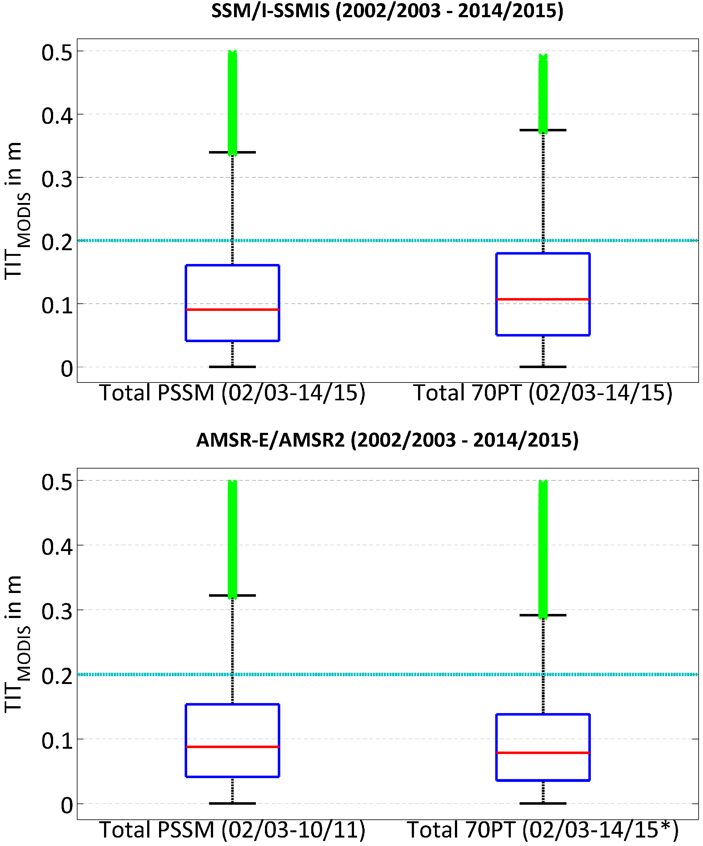
30] for both SSM/I, as well as AMSR-E/AMSR2 for the period 2002 to 2015. We notice that the vast majority of thin-ice pixels in the NOW polynya region as defined by PSSM and 70PT does not exceed the 0.2-m threshold, which is in accordance with previous studies, while at the same time, a significant amount of outliers exists. In the case of PSSM, the average TIT amounts to 11.2 ± 9.0 cm and 10.8 ± 8.6 cm for SSM/I-SSMIS and AMSR-E, respectively. When using a 70% SIC-threshold to derive POLA (70PT), similar values of 12.4 ± 9.1 cm (SSM/I-SSMIS) and 9.7 ± 7.8 cm (AMSR-E/AMSR2) are calculated. As these values are gathered over the complete polynya area as prescribed by PSSM and 70PT, these TIT can be seen as areal averages.
Differences in the retrieved POLA (AMSR-E/2 vs. SMMR/SSM/I-SSMIS 
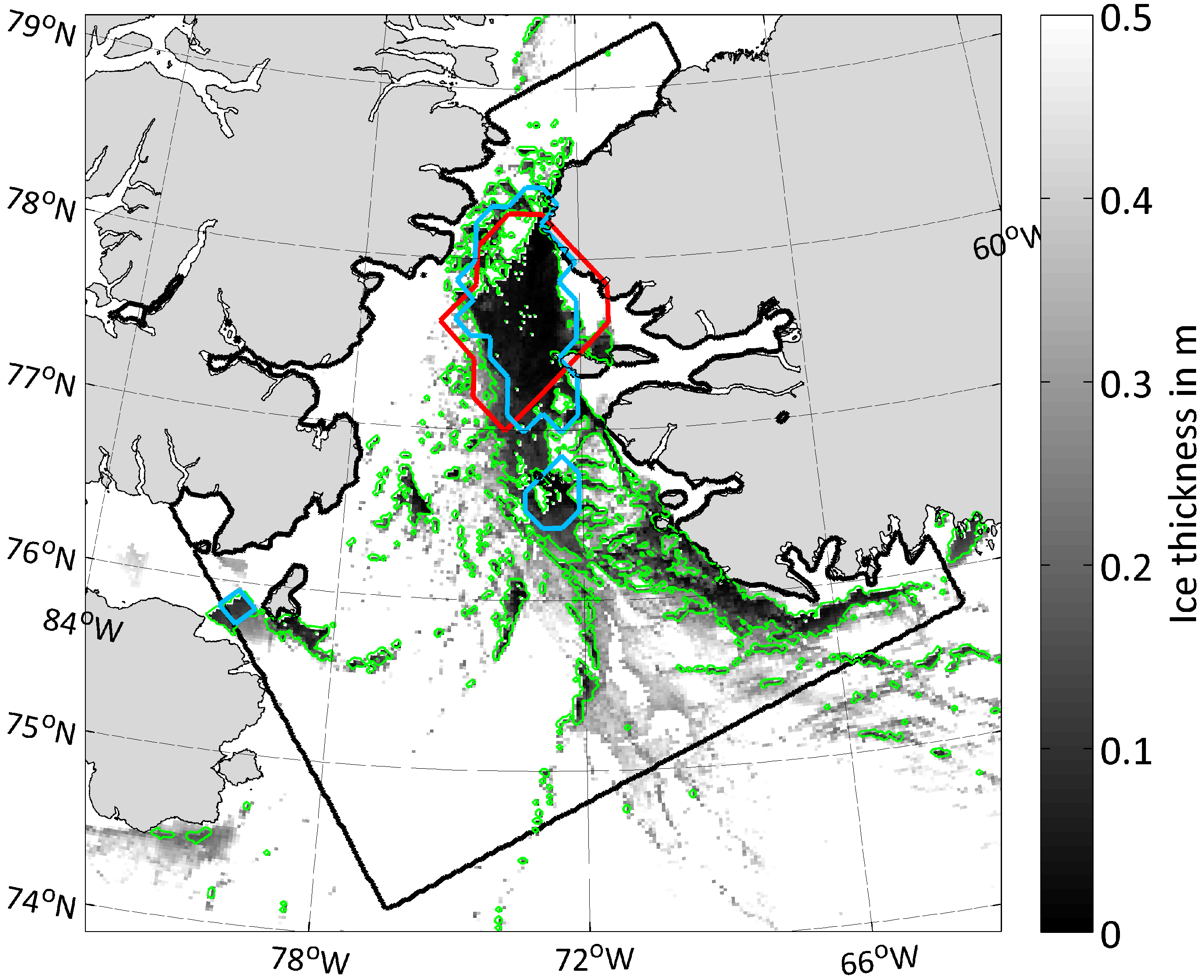
vs. MODIS) can be mostly attributed to the sensor-specific capability to resolve small thin-ice features, such as small coastal polynyas and leads, i.e., the spatial resolution of each sensor. Figure 2 illustrates this effect quite nicely by showing an example (14 March 2009) of the retrieved POLA for MODIS (TIT ≤ 0.2 m; green contour; 2 km), SSM/I 70PT (red contour; 25 km) and SSM/I PSSM (blue contour; 12.5 km). While the passive microwave estimates on that given day are comparable (PSSM: 7463 km 2 ; 70PT: 6691 km 2 ), the MODIS-estimates more than double those values (no CC: 17,804 km 2 ; CC (IST-coverage 92.3%): 19,290 km 2 ).
Figure 3. Box-plots of the daily TIT distribution in polynya areas as detected by passive microwave sensors (upper panel: SSM/I-SSMIS; lower panel: AMSR-E/AMSR2). Boxes on the left side show the MODIS TIT distribution in the PSSM polynya area, while the right-hand boxes show the equivalent information for the 70PT method. The light blue horizontal bar marks the 0.2-m TIT-threshold for the MODIS POLA-retrieval. Red bars indicate the median within the 25th and 75th percentile (inter-quartile range; blue boxes). The whisker length has a default value of 1.5-times the inter-quartile range, and outliers are marked in green (* no AMSR-E/AMSR2 sea ice concentrations available for November to March 2011/2012).
Remotesensing 07 15807 g003

3.2. Assessment of Long-Term POLA Development

As the coarse-resolution SMMR/SSM/I-SSMIS SIC dataset features by far the longest available satellite record (1978 to 2015), 
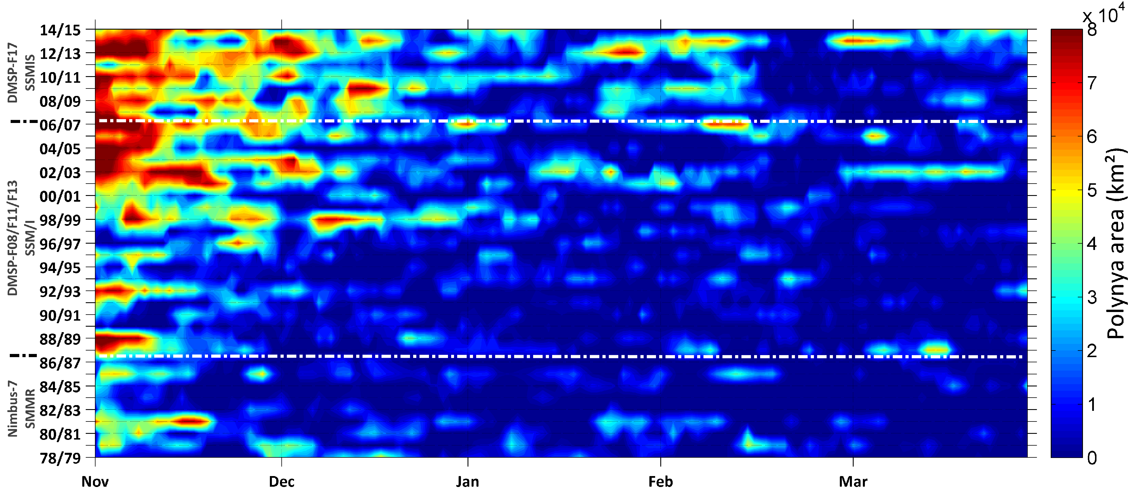
Figure 4 shows the daily development of P O L A S S M I , 70 P T estimates for the NOW polynya. This time series of 37 consecutive winter seasons covers a comparatively long period of time and is therefore better suited for climatological studies than the MODIS and AMSR-E/AMSR2 estimates, which feature only the last 13 winter seasons. It gets clear that the NOW polynya changed significantly during the last three decades, regardless of the absolute accuracy of the underlying SIC dataset [16]. Until the mid-1990s, the overall polynya-activity was very weak. Larger polynya events occurred mainly at the beginning of a freezing season (November), while the remaining months only featured sparse periods with enhanced activity. Overall, a shift to a later fall freeze-up is observed in the last 15 to 16 years, where the polynya exceeds areal extents of 40,000 to 50,000 km 2 until the end of December. In addition, also the remaining months of these years show large polynya events. Less polynya activity is generally observed towards the end of an average winter season.
Figure 4. Hovmöller diagram of daily polynya area ( POLA SSMI,70PT ) in the North Water Polynya between 1978/1979 and 2014/2015. White horizontal dotted lines indicate changing sensors in the sea ice concentration (SIC) dataset by Cavalieri et al. [16].
Remotesensing 07 15807 g004
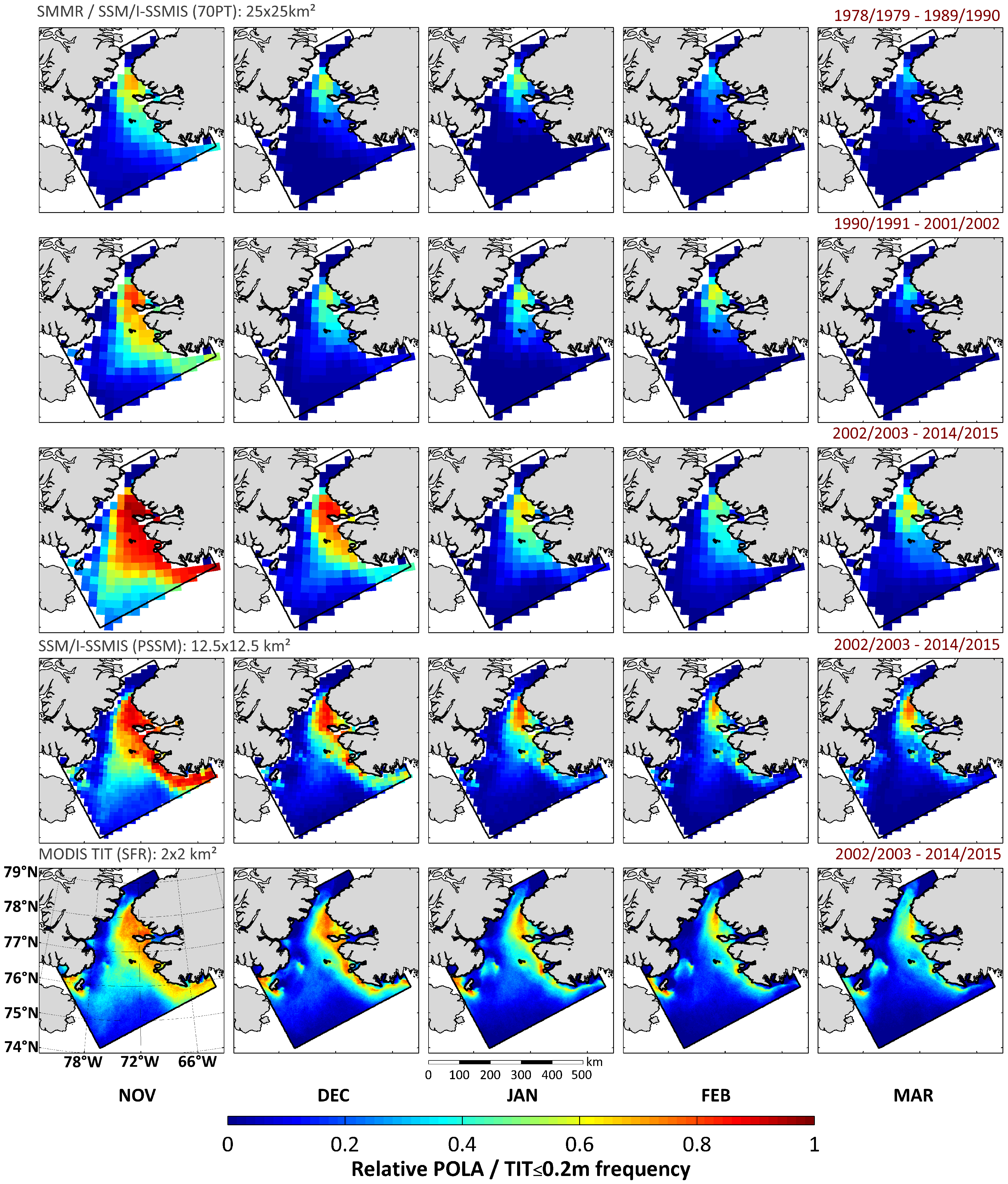
Figure 5 shows spatial overviews of the relative frequency of polynya/thin-ice occurrences on a monthly basis (November to March) based on daily P O L A S S M I , 70 P T estimates, P O L A S S M I , P S S M estimates and MODIS TIT (using SFR for gap filling). The upper three rows roughly represent the 1980s (1978/1979 to 1989/1990), the 1990s (1990/1991 to 2001/2002) and the 2000s (2002/2003 to 2014/2015) periods to detect decadal changes of the sea ice in northern Baffin Bay. The lower two rows show equivalent information for the 2000s period based on P O L A S S M I , P S S M and MODIS. In the 1980s, the NOW polynya features an overall low activity. These first 12 winter seasons show appearance rates of around 70% (21 d) in November down to approximately 30% (9 d) in February and March in the area of Smith Sound. The main polynya activity during this period is limited to areas north of 76 N (maximum extent in November). During the 1990s and even more the 2000s, this region vastly expands down to approximately 74 N. Even in January to March, appearance rates of over 20% to 30% extend down to around 76 N. Remarkably, the monthly duration of the polynya in the proximity of Smith Sound increases towards 60% (17 to 19 d) in January to March and up to 90% to 100% (28 to 31 d) in November to December. The finer resolving counterparts from MODIS, SSM/I-SSMIS (PSSM) (Figure 5; 2000s period) and AMSR-E/AMSR2 (not shown) are certainly able to provide more precise regional differentiations. Not only in the case of MODIS (relative frequencies of TIT ≤ 0.2 m), observed patterns are in accordance with earlier studies (e.g., [8,20,21]) and underline the previously-stated observations based on coarse-resolution SMMR and SSM/I-SSMIS 70PT data. In addition, the detection of small-scale features, like the clearly visible shape of the ice bridge at Smith Sound, as well as larger thin-ice areas at the eastern side of the polynya, profits from the enhanced spatial resolution of MODIS. Also noticeable is a quite large area with values ranging from around 35% to 60% south of Ellesmere Island (eastern entrance of Jones Sound).
Figure 5. Average monthly relative frequency distribution of polynya-pixels as classified by the 70PT-method (SMMR/SSM/I-SSMIS; top three rows), the PSSM method (SSM/I-SSMIS); fourth row) and based on MODIS thin-ice thicknesses ≤ 0.2 m (daily TIT composites with applied spatial feature reconstruction (SFR); bottom row). Note the reference period over which the monthly relative frequency distributions are calculated, as indicated in the the upper right corner of each row.
Remotesensing 07 15807 g005
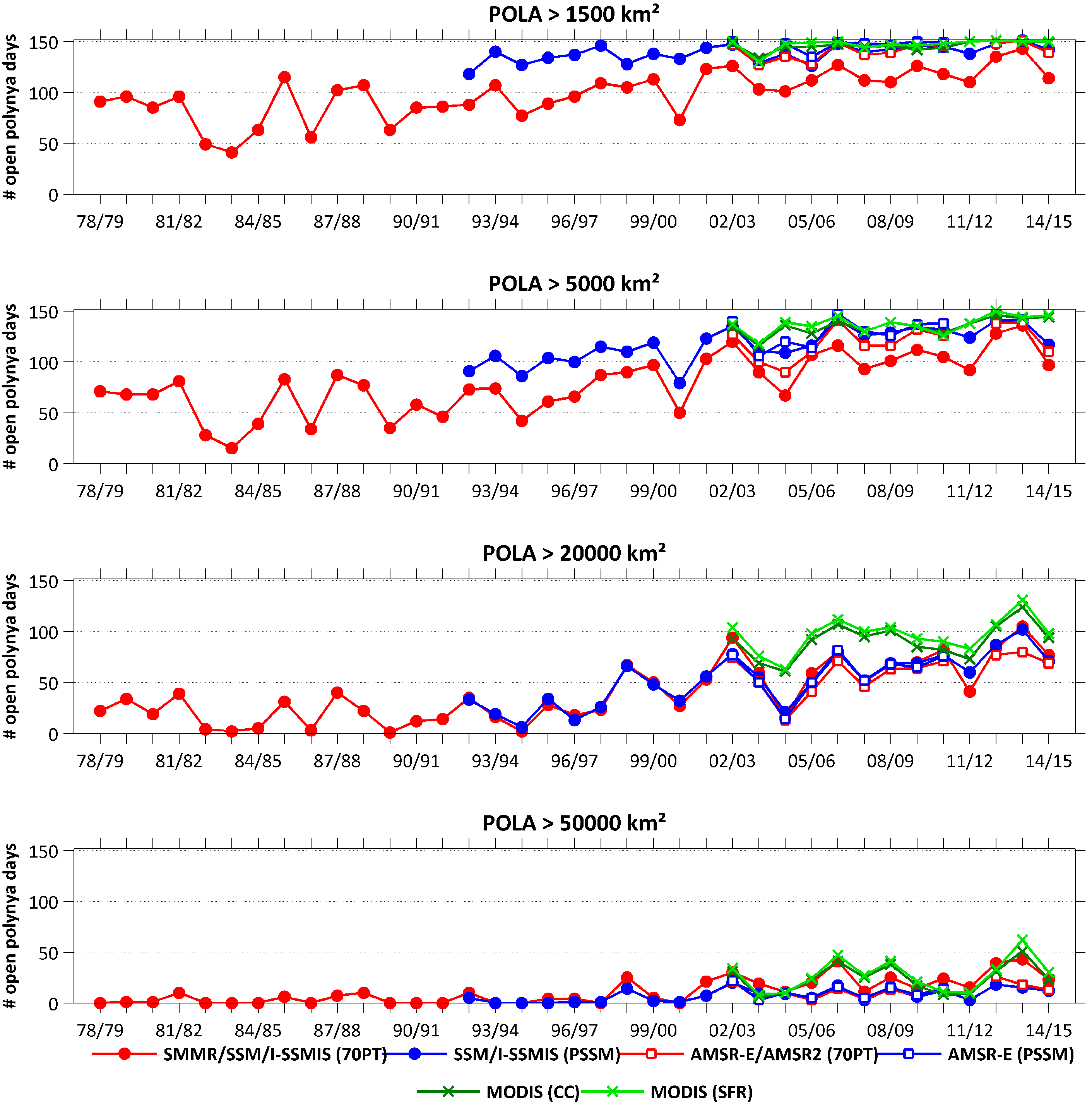
Figure 6 sums up the previous findings for the whole regarded period from 1978 to 2015. It shows the amount of open polynya days (based on POLA estimates from MODIS (CC/SFR), AMSR-E/AMSR2 and SMMR/SSM/I-SSMIS (both 70PT/PSSM)) exceeding a certain areal threshold (POLA ≥1500/5000/20,000/50,000 km 2 ). In the upper panel (POLA ≥1500 km 2 ), days that are falling below a threshold of 1500 km 2 , i.e., an almost closed polynya, can be depicted by the difference of given values to the total number of days each winter season (November to March; 151/152 d). In recent winters, the number of very small to almost closed polynyas seems to vanish almost completely (except for the SMMR/SSM/I-SSMIS 70PT retrievals). On the other hand, the number of larger polynyas increases significantly from approximately 1997/1998 onwards, especially those exceeding a threshold of 20,000 km 2 . Noteworthy is the higher amount of detected polynyas larger than 20,000 km 2 from MODIS and a good agreement between MODIS and the passive microwave estimates for very large polynyas (≥50,000 km 2 ).
Figure 6. Number of polynya days with an area of ≥1500 km 2 , ≥5000 km 2 , ≥20,000 km 2 and ≥50,000 km 2 within the applied polynya mask. A comparison is made between POLA estimations based on daily MODIS TIT composites (CC: dark green crosses; SFR: light green crosses) and passive microwave sensors (SMMR/SSM/I-SSMIS 70PT: filled red circles; AMSR-E/AMSR2 70PT: unfilled red squares; SSM/I-SSMIS PSSM: filled blue circles; AMSR-E PSSM: unfilled blue squares). The numbers indicate the amount of polynya days for each area threshold from zero.
Remotesensing 07 15807 g006
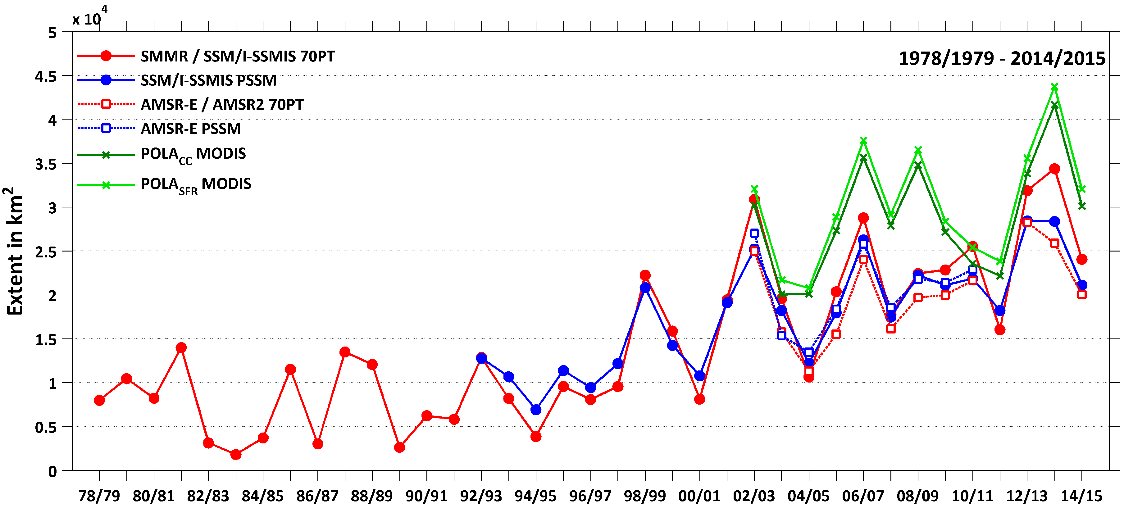
A comparison of the wintertime mean POLA for all available sensors and retrieval-schemes is presented in Figure 7 for the complete record of 37 winter seasons. In this long-term context, we find coherent patterns between all incorporated satellites and sensors, although absolute mean values are differing. Further, a tendency towards larger areal extents of the NOW polynya becomes very obvious. As could be seen before, the winter seasons around 1996/1997 to 1997/1998 seem to be the periods where the NOW polynya starts to expand from an average level of around 7000 km 2 in the 1980s and early 1990s up to almost doubled average values in recent years.
Figure 7. Average wintertime (November to March) polynya area (POLA) for the period from 1978/1979 to 2014/2015. A comparison is made between POLA estimations based on daily MODIS TIT composites (CC: dark green crosses; SFR: light green crosses) and passive microwave sensors (SMMR/SSM/I-SSMIS 70PT: filled red circles; AMSR-E/AMSR2 70PT: unfilled red squares; SSM/I-SSMIS PSSM: filled blue circles; AMSR-E PSSM: unfilled blue squares).
Remotesensing 07 15807 g007
This sudden “POLA shift” during the mid-1990s may be related to the clear warming trend in northwestern Greenland from 1994 onwards [41] (associated with an increasing amount of blocking events (high-pressure anomalies) over the Greenland Ice Sheet (GrIS), e.g., [42]). The North Atlantic Oscillation (NAO) and Arctic Oscillation (AO) are well known and widely used indices that characterize large-scale atmospheric variability in the Northern Hemisphere. While featuring significant interannual and seasonal variability, the NAO experienced a transition to a prevailing more negative phase in 1995/1996, which so far peaked in the most negative wintertime NAO index in 2009/2010 [43]. These negative phases are associated with a high-pressure anomaly/ridges over the GrIS, which can bring relatively warm southerly winds from lower latitudes to the western side of Greenland [44]. Although the NAO and AO are very similar from a conceptual point of view and do strongly correlate (r > 0.8), the recently declining nature of the summer NAO is not replicated in the AO index [45]. Instead, both indexes show enhanced wintertime variability in recent years [45,46]. However, extreme negative phases, like in 2009/2010, are evident in both the NAO and AO index. Stroeve et al. [46] highlights that winter months (December to January) for the period 1979 to 2009 with a strongly negative AO index tend to show positive air temperature (925-hPa level) anomalies and negative SIC anomalies over Greenland, Baffin Bay, Canada and Alaska. A steady increase in autumn and winter air temperatures from 1995/1996 onwards could slow down or limit ice growth during freeze-up and, hence, lead to prolonged periods with very thin ice in northern Baffin Bay. Following this argumentation, increasing POLA and a later fall freeze-up align well. Therefore, besides having a potentially large influence on summer melt rates on the GrIS and land surface [41], we assume that increased winter warming and associated negative NAO phases are also linked to sea ice and polynya characteristics in the NOW region.
Overall, it can be noted, that MODIS, as well as both AMSR-E PSSM and SSM/I-SSMIS PSSM all capture the general seasonal development of polynya opening events in good agreement (compare Table 3). In several cases, MODIS-derived POLA exceeds the passive microwave estimates by a factor of 1.5 to two, especially for polynyas below 40,000 km 2 . When comparing individual winter seasons, a large interannual variability can be observed.
Table 3. Comparison of calculated monthly mean polynya area (POLA; in 10 3 km 2 ) from different sensor types (SSM/I-SSMIS, AMSR-E, MODIS) and methods, averaged over the overlapping period from 2002/2003 to 2010/2011 (November to March). Cloud-cover corrections have been applied to the MODIS data where CC denotes the values after coverage correction and SFR denotes the values after the spatial feature reconstruction (compare Section 2.6). All values are calculated within the predefined polynya mask (Figure 1).
SSM/I-SSMIS 70PT (10 3 km 2 )SSM/I-SSMIS PSSM (10 3 km 2 )AMSR-E70PT (10 3 km 2 )AMSR-EPSSM (10 3 km 2 )MODISCC (10 3 km 2 )MODISSFR (10 3 km 2 )
November50.539.338.539.139.342.8
December25.621.620.522.529.030.8
January12.915.613.515.326.928.1
February11.412.610.813.521.822.5
March10.012.210.512.119.920.3
Mean22.120.318.820.527.428.9
SD17.011.311.811.27.68.8

3.3. Thin-Ice Thickness Distribution and Thermodynamic Ice Production for 2002/2003 to 2014/2015

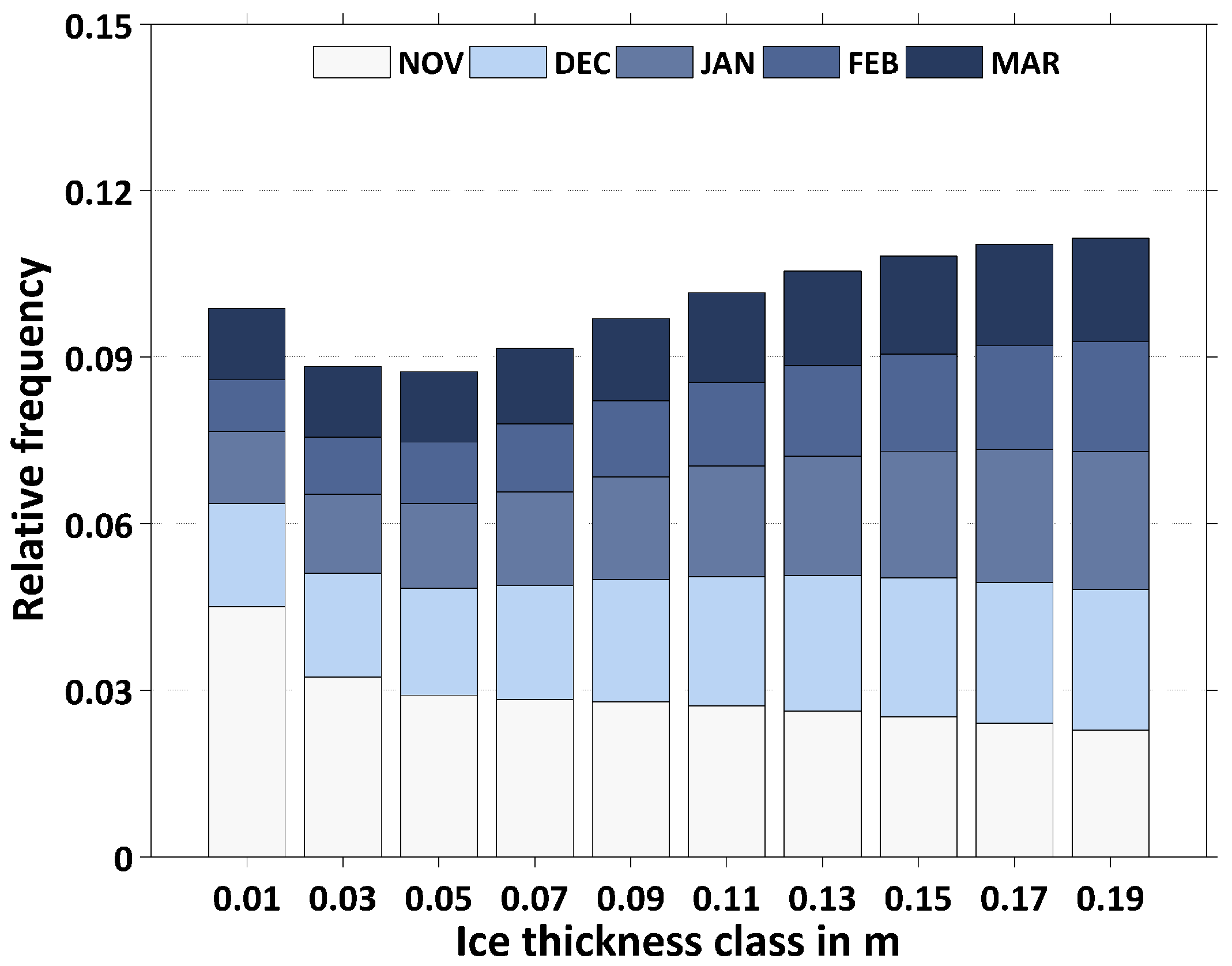
Figure 8 shows a histogram of the total wintertime relative TIT distribution for ice thicknesses below 0.2 m, based on median daily composites. Colors indicate monthly differences. Between November and March, ice thinner than 0.04 m contributes around 9 to 10% to the total polynya area in an average winter season, with the largest proportion being present in November during freeze-up. Thicker ice classes (>0.1 m) show higher contributions of around 10 to 11% in total, therefore covering more than half of the entire NOW polynya predominately from January to March. Concerning the thin-ice thickness distribution in the NOW-polynya region, there is only sparse information available in recent literature. As Ingram et al. [5] states, an improved characterization of the ice-thickness distribution is one of the main aspects that needs to be further investigated in the NOW region to get more viable information about the magnitude of heat exchange between ocean and atmosphere. Nevertheless, some information on sea ice types and associated ice thicknesses in the North Water region can be found in an older study by Steffen [47]. This study had the purpose of investigating the general ice conditions in the winters of 1978/1979 and 1980/1981 by means of an aerial survey performing radiometric temperature measurements of the sea surface. From these measurements, distinct ice types were classified, and their proportion to the sea ice cover was derived. According to Steffen [47], more than 50% of the NOW polynya (in his study called “Smith Sound polynya”) was covered by young ice (0.1 m to 0.3 m), nilas (0 m to 0.1 m) and open water in the months November to January. This is roughly in accordance to the estimated relative TIT frequencies (TIT ≤ 0.2 m) for November to December derived in this study, where values up to 65% are visible south of Smith Sound. Steffen [47] also states that in February and March, more white ice (>0.3 m) was present during their flight campaigns. This fits the conclusion made earlier that there is less polynya activity in the NOW region towards the end of the freezing season (Figure 4 and Figure 5). While there is no direct comparison available for the TIT distribution shown in Figure 8, the study of Steffen [47] also gives an indication that the derived proportion of very thin ice is not far off from his observations (see his Table 3; categories “ice-free” and “dark nilas” combined), despite a possible bias in this thickness class due to inherent cloud and sea smoke effects [36].
Figure 8. Histogram of the relative thin-ice thickness (TIT) distribution in the NOW polynya, with ice-thickness classes of the 2-cm range (x axis). Input data are based on daily TIT composites covering the complete freezing season from November to March. The bars indicate the relative distribution of each thickness class from the total number of TIT ≤ 0.2-m appearances between the winter seasons 2002/2003 and 2014/2015. Contributions of each month with respect to the whole winter season for each thickness class are indicated by the blueish colors (see the legend).
Remotesensing 07 15807 g008
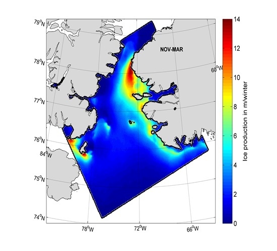
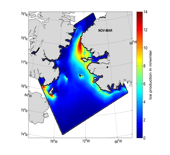
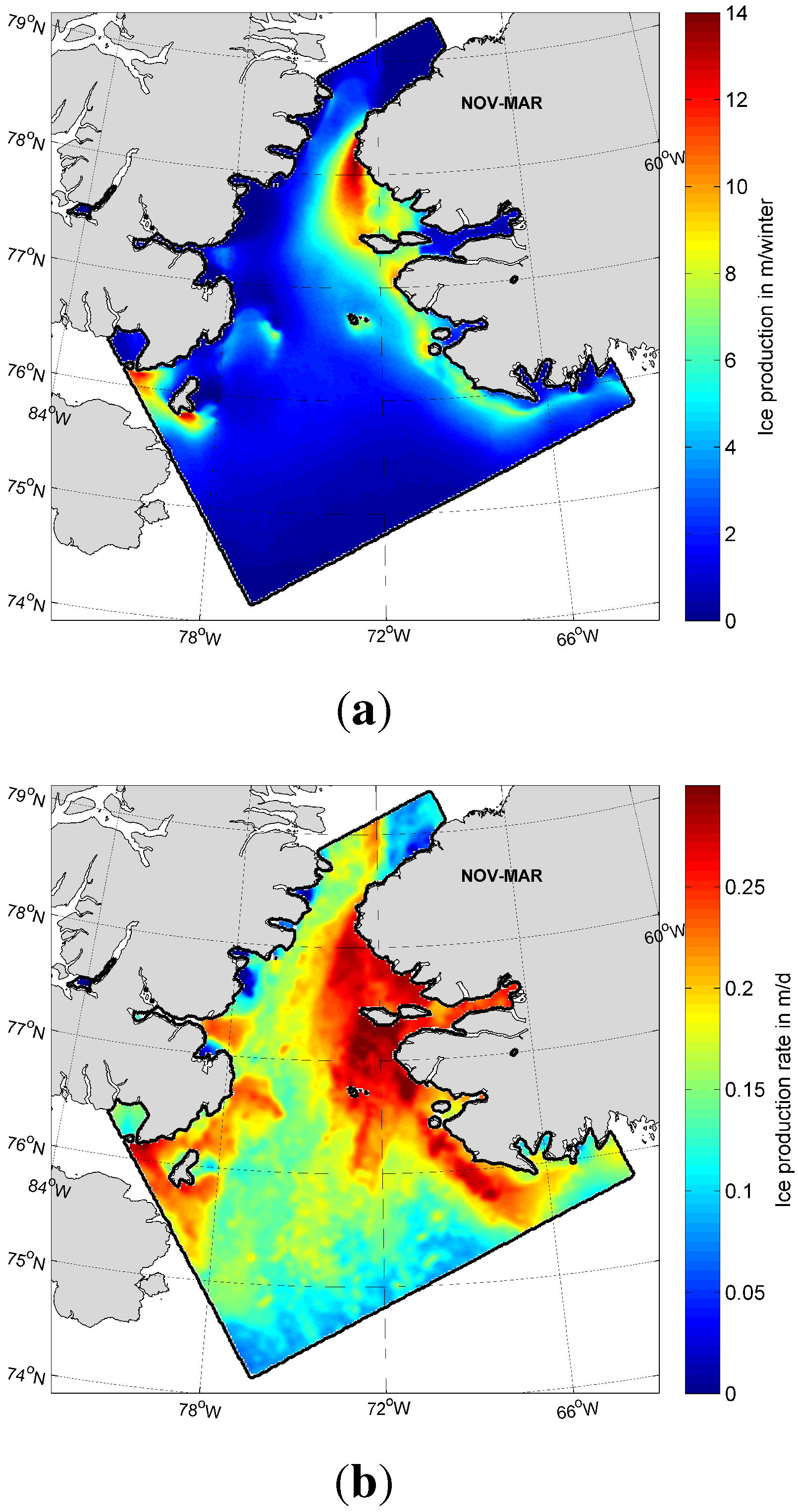
Based on the calculated thin-ice distributions, daily averaged net surface heat loss and associated ice production (rates) are pixel-wise calculated. Spatial overviews of interannual (2002/2003 to 2014/2015) average wintertime ice production (in m·winter - 1 ) and the daily maximum ice production rates (in m·d - 1 ) are shown in Figure 9 with the purpose of locating regional differences and typical spatial patterns. The highest values of accumulated ice production (up to 13 to 14 m·winter - 1 ; Figure 9a) occur directly south of the Greenland side of Smith Sound (lee-side) and slightly lower values (around 5 to 8 m·winter - 1 ) in proximity of the West Greenland coast. These values compare well to Iwamoto et al. [21], who state a maximum rate of 13 m·winter - 1 and are therefore lower than the 19 m·winter - 1 stated by Tamura and Ohshima [20]. Maximum daily rates at these locations can exceed 20 to 25 cm per day, in certain areas even reaching values as high as 30 cm per day (e.g., south of Northumberland Island at approximately 77 N, 72 W; Figure 9b). It has to be noted that the typical location of the ice bridge at Smith Sound (see the following Section 3.3) is well visible and recognizable by its characteristic arch-like shape. However, the main location for high ice formation rates is found at the eastern exit of Smith Sound, indicating the importance of the gap flow dynamics for the polynya formation in that area [48]. Other prominent features are large areas of high ice production between Ellesmere Island and Devon Island in the west of the polynya domain near Coburg Island. While potentially belonging to individual smaller polynya systems (as implied by Barber and Massom [1]), these areas are included in our NOW polynya estimates.
Figure 9. Spatial distribution of (a) the average accumulated ice production (IP, in m·winter - 1 ) rate, as well as (b) the maximum daily ice production rate (in m·d - 1 ) in the North Water Polynya for winter seasons (November to March) 2002/2003 to 2014/2015.
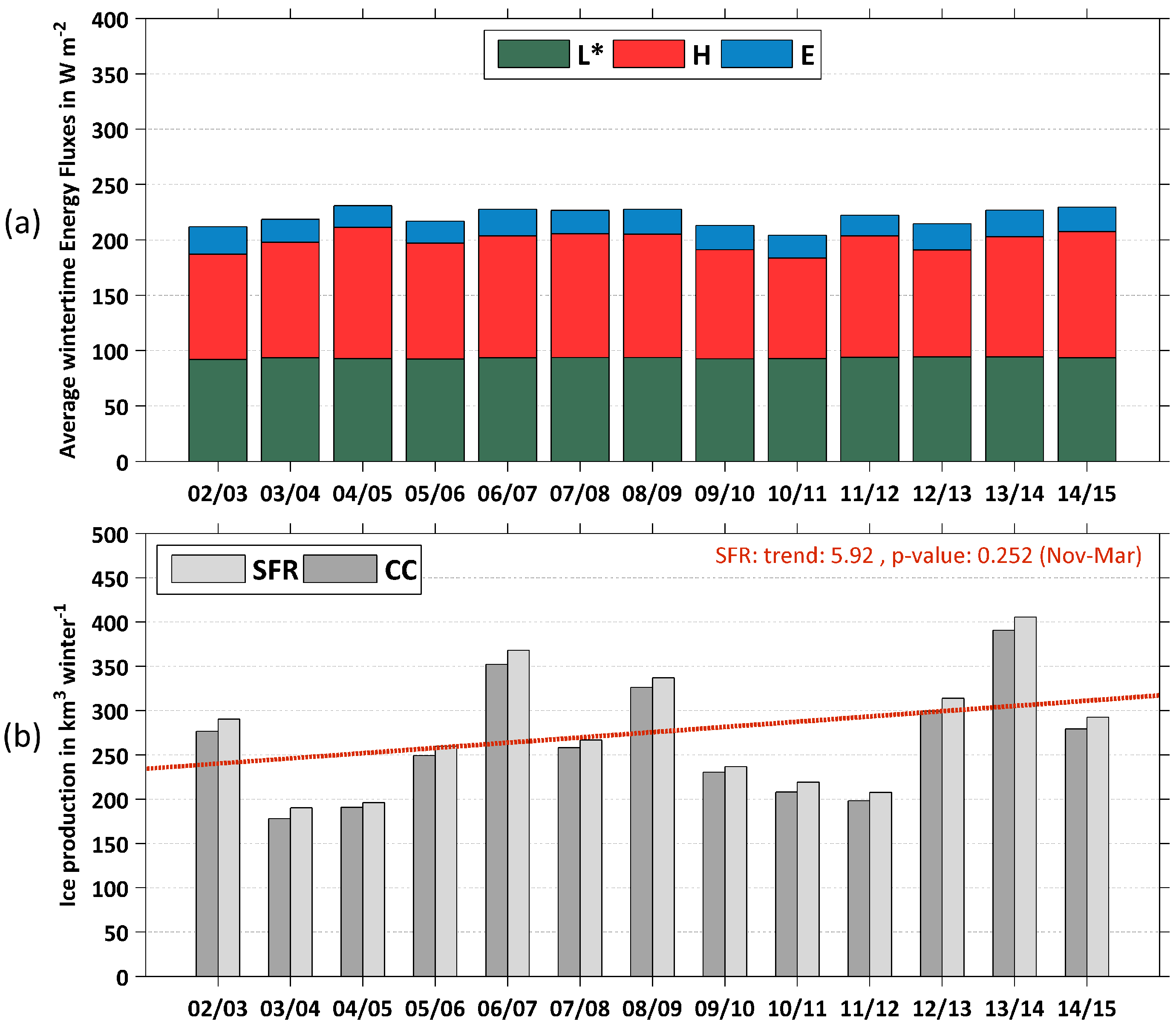
Remotesensing 07 15807 g009
In Figure 10a,b, average wintertime energy fluxes from the heat flux calculations are shown together with the total accumulated ice production (CC/SFR) per winter season from November to March. A detailed overview on ice production and polynya area (CC/SFR) for each winter season is additionally given in Table 4. Overall, the average fluxes from both net long-wave radiation and latent heat show almost no interannual variability by ranging around 95 W·m - 2 and 25 W·m - 2 , respectively. The net energy balance during wintertime is therefore strongly controlled by the contribution of the sensible heat flux. In the NOW region, average values for H are ranging between 91 W·m - 2 (2010/2011) and 119 W·m - 2 (2004/2005). Concerning wintertime ice production in the NOW polynya, results from the two correction schemes (CC/SFR) are overall differing by approximately 4%. The average IP SFR value amounts to 275.7 ± 67.4 km 3 (CC: 264.4 ± 65.1 km 3 ). We note a high interannual variability of ice production, with values as low as 190.2 km 3 (SFR; CC −6.9 %) in 2003/2004 and up to 405.7 km 3 (SFR; CC - 3 . 9 %) in 2013/2014. Large increases in IP occur from winter 2005/2006 to 2006/2007 (SFR: +108 km 3 ) and again from winter 2011/2012 to 2012/2013 (SFR: +106 km 3 ). Regardless of the applied cloud-cover correction, a non-significant positive trend of 5.9 km 3 ·yr - 1 can be observed over the examined 13 winters’ record. The high ice production in 2013/2014 can be partly explained by continuously high frequencies of TIT 0 . 2 m and, therefore, several large polynya events in the NOW area throughout the whole winter season from November to March.
Figure 10. (a) Average wintertime (November to March) energy fluxes of net long-wave radiation (L*), sensible (H) and latent (E) heat (all in W·m - 2 ) within the applied polynya mask. (b) Annual wintertime accumulated ice production (IP) in the NOW polynya (in km 3 ·winter - 1 ) for 2002/2003 to 2014/2015. Estimations of IP are based on heat flux calculations using the daily derived TIT composites. Special emphasis is given to the effect of an applied cloud-cover correction (CC/SFR). The red dotted line shows a linear trend estimation for IP SFR .
Remotesensing 07 15807 g010
Table 4. Accumulated ice production in km 3 per winter and average polynya area (in 10 3 km 2 ) for each winter season (November to March) from 2002/2003 to 2014/2015 in the North Water Polynya, together with the interannual average (mean) and its standard deviation (SD). Cloud-cover corrections have been applied where CC denotes the values after coverage correction and SFR denotes the values after the spatial feature reconstruction (see the text). All values are derived from daily MODIS TIT composites after application of the predefined polynya mask (Figure 1).
Acc. IP CC (km 3 )Acc. IP SFR (km 3 ) POLA CC (10 3 km 2 ) POLA SFR (10 3 km 2 )
2002 to 2003276.6290.330.232.1
2003 to 2004178.0190.220.021.7
2004 to 2005191.0196.220.120.8
2005 to 2006249.2259.827.328.8
2006 to 2007352.2368.235.637.6
2007 to 2008258.2266.627.929.1
2008 to 2009326.2337.134.836.5
2009 to 2010230.5236.727.228.3
2010 to 2011208.1219.123.525.4
2011 to 2012198.3207.822.223.8
2012 to 2013299.4313.933.835.6
2013 to 2014390.6405.741.743.7
2014 to 2015279.1292.630.132.0
Mean264.4275.728.830.4
SD65.167.46.56.7
Comparative numbers from previous studies in terms of ice production are hard to find for the NOW polynya. There are recent studies by Tamura and Ohshima [20] (hereafter TO11) and Iwamoto et al. [21] (hereafter I14), who both estimated pan-Arctic ice production in polynyas. Their estimated ice production values are based on newly-developed thin-ice algorithms, which use either SSM/I or AMSR-E brightness-temperature data to calculate thin-ice thicknesses. These algorithms are based on empirical approaches, which incorporate either Advanced Very High Resolution Radiometer (AVHRR) or MODIS-calculated reference-thicknesses (TIT). Similar to our study, these estimated ice thicknesses are then combined with heat-flux calculations (NCEP2 [49]/ERA-Interim reanalysis serving as the atmospheric dataset) to achieve ice production.
For the NOW polynya, TO11 [20] and I14 [21] state an average ice production of 353 ± 69 km 3 (1992/1993 to 2007/2008) and 186 ± 34 km 3 (2002/2003 to 2010/2011), respectively. The base-period of these studies is extended by four months each winter season compared to our study (November to March), and the applied polynya masks are differing (similar to the comparisons in [32]), which makes direct comparisons challenging. For the same averaging interval as I14 and based on IP SFR , we achieve a 41% higher value of 263 ± 61 km 3 . We assume that the values derived here are more accurate, as they profit from the enhanced resolution of MODIS. Additionally, they are presumably far less influenced by ambiguities in heat loss calculations by leaving out the months of September, October, April and May. Regarding the large ice production in TO11 [20], the study of I14 [21] refers to a “thin-bias”, which is explained by differences in the applied atmospheric reanalysis data (NCEP2 vs. ERA-Interim). Thereby, larger calculated heat loss and thinner TIT are explained by a lower bias in 2-m-air temperature and a higher bias in wind speed when NCEP2 is compared to ERA-Interim in the the Arctic Ocean domain (also evident in Lindsay et al. [50]). Part of the difference from I14 is thought to originate from a smaller areal extent of their polynya mask, which excludes the area of high IP at the eastern entrance of Jones Sound (around 76 N, 81 W; compare Figure 9). We also applied a smaller polynya mask, which excluded the Jones Sound area for earlier investigations on the NOW polynya, which resulted in slightly lower IP (CC) estimates (about 8%). Taking this into consideration, our presented average accumulated IP values would get closer to I14, while still being higher.
Both TO11 and I14 [20,21] state that polynyas located around the Canada Basin (including the NOW polynya) show the largest ice production values in the early stage of the freezing period (October to December), which afterwards gradually decrease towards March. This is also revealed in our data and can be explained by more consolidated pack ice in northern Baffin Bay and several fast-ice areas around Ellesmere Island at the end of a freezing season, which limit the west- and south-ward expansion of the NOW polynya.

3.4. Ice Bridge Dynamics in Nares Strait (2002/2003 to 2014/2015)

According to Kwok et al. [51], ice bridges typically form at two distinct locations along Nares Strait. A deeper understanding of the involved mechanisms and temporal patterns is of high value, as the movement of sea ice through Nares Strait and, therefore, the export of old multi-year ice from the north of Greenland is strongly controlled by the timing and location of ice bridge formation.
In the context of the present study, the most prominent location is certainly Smith Sound at the southern exit of the channel, as it usually is associated with the formation of the NOW polynya (e.g., [5,8]). According to Barber et al. [8], the timing of wintertime ice bridge formation at Smith Sound is quite variable by occurring sometime between November and March. Barber et al. [8] analyze time series of SIC north and south of the typical ice bridge location to infer characteristic development stages in the course of a year. While a similar analysis using our data worked reasonably well for the southern ice bridge at Smith Sound, we were not able to apply this analysis to the northern ice bridge locations at Robeson Channel (compare Figure 1), presumably due to the coarse resolution of the passive microwave data.
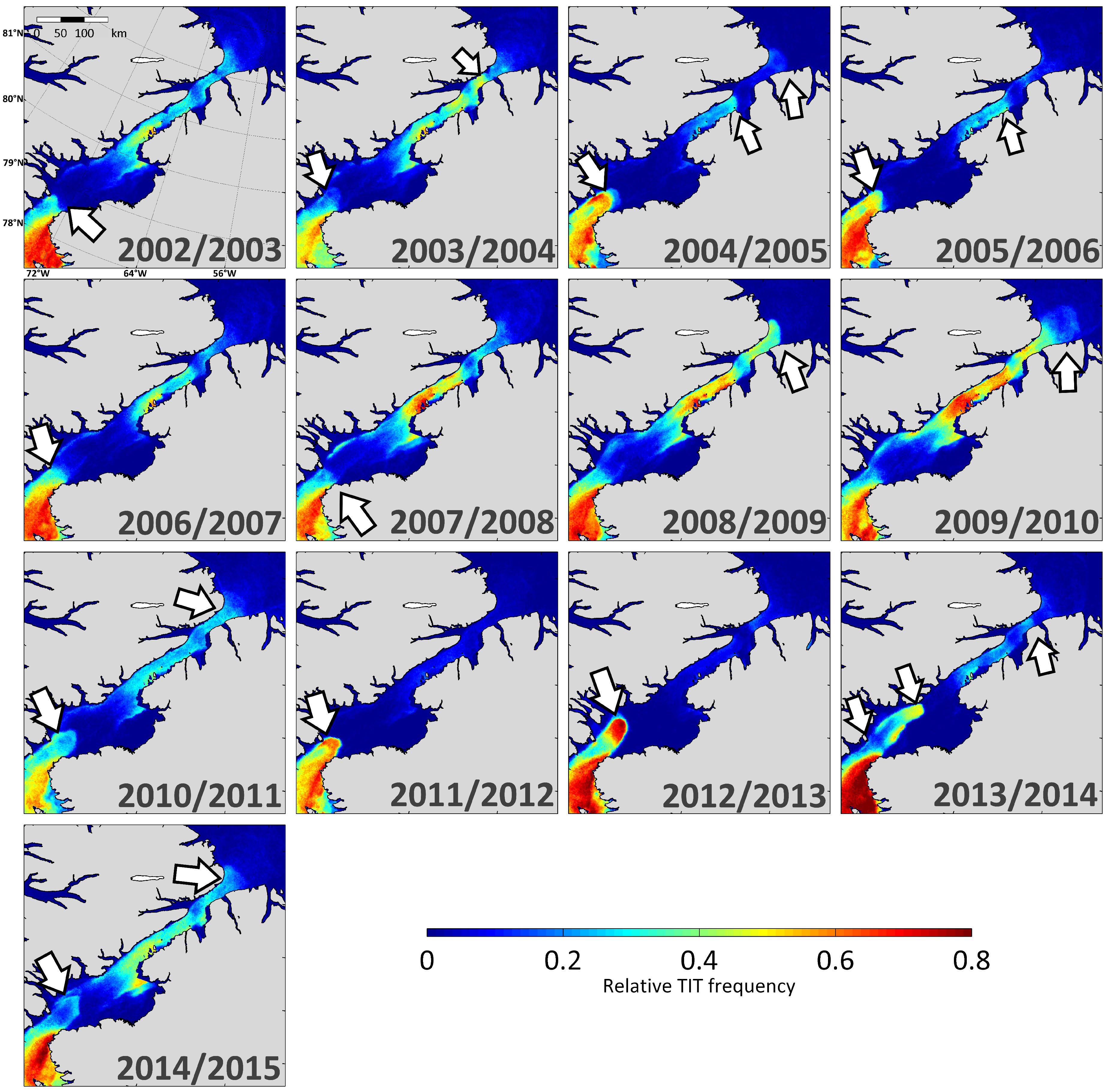
As an alternative approach we decided to take a closer look at the annual (November to March; 151/152 days in total) relative occurrences of MODIS TIT ≤ 0.2 m, in order to relate typical thin-ice locations to nearby ice bridge patterns. The spatial overviews for the winter seasons 2002/2003 to 2014/2015 are presented in Figure 11. The observed locations of an arch-type pattern during each winter season are marked with a white arrow. The southern ice bridge at Smith Sound is present in every winter season, except the period from 2008/2009 to 2009/2010. Contrary to Kwok et al. [51], who also had a closer look at the behavior of the ice bridges in Nares Strait, we cannot confirm the absence of the southern ice bridge in 2006/2007, which was stated as the main reason for a sea ice export anomaly through Nares Strait in 2007. It was assumed that the movement of sea ice was not suppressed by any kind of blocking features both at Smith Sound in the south and Robeson Channel roughly 450 km further north. While the latter is also observable in our study (high TIT frequencies in the northerly part of Nares Strait), an arch-type TIT pattern at the southern end of Nares Strait was present during the whole winter season from November to March, although its location is very variable. In addition, daily TIT maps reveal several events where large patches of ice broke off at Smith Sound and drifting further south, thereby still indicating a less stable ice bridge and enhanced sea ice export at the Canadian side of the channel.
Figure 11. Relative frequency distribution of thin-ice thickness ≤ 0.2 m in northern Baffin Bay/Smith Sound, Nares Strait and Lincoln Sea for the complete freezing seasons (November to March) 2002/2003 to 2014/2015, based on daily TIT composites. Observed sites of ice bridge appearances between November and March are indicated by white arrows.
Remotesensing 07 15807 g011
Barber et al. [8] stated that the formation of an ice bridge at Smith Sound seemed to be less regular in the 1990s compared to the 1980s, with a tendency to form later and break up earlier. As we only regard the case of ice bridge formation during winter, we cannot comment on the timing of ice bridge break-up for the 2000s and ongoing. Regarding the later appearing ice bridge formation, we noted a large monthly variability of TIT frequencies in Nares Strait over the last 13 winter seasons, but no sign of a temporal shift.
Using SAR (Synthetic Aperture Radar) satellite imagery from RADARSAT, Kwok et al. [51] estimated the average timing of ice bridge formation at Smith Sound to be around 2 February (±44 d), blocking the ice movement in Nares Strait on average for 184 ± 10 d until the summer melt period. Based on monthly TIT frequency distributions (2002/2003 to 2014/2015; not shown), we can confirm that the most regular ice bridge development starts from February onwards. In addition, more than half of the winters between 2002/2003 and 2014/2015 already feature an ice bridge in November and December.
Unfortunately, we are not able to directly relate the ice bridge formation in Nares Strait to the development of the NOW polynya during winter. Years with high wintertime POLA and IP do not necessarily coincide with long ice bridge periods and vice versa. Hence, we expect that the ice bridge at Smith Sound becomes more important around April to June, when the NOW-polynya starts to expand southward.

4. Summary and Conclusions

In this study, we present a long-term analysis of polynya dynamics and ice production in the NOW polynya for the winter seasons 1978/1979 to 2014/2015. For that purpose, we analyzed remote sensing data from both passive microwave (AMSR-E, AMSR2, SMMR/SSM/I-SSMIS) and thermal infrared (MODIS) sensors to infer characteristic polynya quantities, such as the total polynya area (POLA) and thermodynamic ice production (IP), on various spatial resolutions and temporal scales. In order to allow comparisons between MODIS and passive microwave estimates, two well-working approaches are applied to overcome difficulties with falsely-classified and/or undetected cloud-covered pixels. All sensors capture the overall seasonal development of the polynya very well, with differences occurring mainly in terms of polynya sizes due to the varying capability to resolve smaller thin-ice features. Thereby, daily POLA derived by MODIS exceeds the passive microwave estimates in most cases, as leads and areas in close proximity to the coasts of Greenland and Ellesmere Island contribute to the estimations. This results in about 30 to 40% higher average POLA estimates compared to the ones derived by AMSR-E. MODIS estimates can even exceed the POLA values derived by SSM/I, depending on the type of calculation (70PT/PSSM). In addition, land spillover effects are reduced compared to coarse-resolution passive microwave estimates of POLA, which is especially valuable for areas with a very rugged coastline, such as Greenland. While the difference in POLA between the 70PT and PSSM approach is fairly low (approximately 10%) for AMSR-E, it can be much larger for the coarse-resolution SSM/I-SSMIS data, especially in November and December, when large thin-ice areas dominate the NOW region. As a compromise between a long-term satellite record and a good agreement with the comparatively high-resolution MODIS estimates, the PSSM method should be used instead of the 70PT method with SSM/I-SSMIS data to calculate POLA over longer time scales.
Compared to earlier studies in the NOW polynya region, the results presented in this study extend the time series and use a multi-sensor approach. The derived location of predominant thin-ice occurrences (i.e., POLA) is in accordance with other studies and focuses on the Smith Sound area with ice bridge and gap flow mechanics as the responsible formation mechanisms. Our results confirm earlier observations by Steffen [47] regarding high polynya activity at the beginning of the freezing period and less polynya activity towards the end of the freezing season and give new insights on a steady increase in polynya area since the mid-1990s. We suggest a potential connection of this sudden shift to a predominately negative phase of the NAO since 1995/1996. However, a more detailed analysis on this topic is beyond the scope of this study and should be implemented in a future atmospheric study. Comparative numbers for the ice production in the NOW polynya are given in Tamura and Ohshima [20] and Iwamoto et al. [21]. Their estimations derived from coarse-resolution SSM/I and AMSR-E data are either by far higher [20] than the results presented here from MODIS IST data or clearly lower [21], which is (at least to some extent and also considering an apparent “thin-bias” in [20]) expected to originate from the shortened investigation period in this study (leaving out September, October, April and May) and different polynya masks [21].
Increased thin-ice frequencies in Nares Strait could be linked to nearby ice bridge formation by revealing distinct spatial patterns. Unfortunately, we could not deduce a clear relation to our calculated polynya metrics and instead assume an increased importance of the ice bridges in Nares Strait towards spring and summer.
Long-term time series of POLA (1978/1979 to 2014/2015) and IP (2002/2003 to 2014/2015), as well as thin-ice characteristics in Nares Strait complement atmospheric and oceanographic observations and model efforts in the NOW region over the last decades. A future synthesis of atmospheric and oceanographic modeling and remote sensing observations might help to explain the obvious changes that are taking place in the NOW region since the 1990s and ongoing. Although the atmospheric part is the essential formation mechanism for the NOW polynya, e.g., [5,8,20], a more detailed analysis of the ocean heat budget (influenced by the Arctic ocean and different water masses in Baffin Bay, like the relatively warm West Greenland Current [11]) and potential implications could certainly help to obtain a complete picture. Supplementary data are available at http://dx.doi.org/10.1594/PANGAEA.854921.

Acknowledgments

The authors want to thank the National Snow and Ice Data Center (NSIDC), as well as the European Center for Medium-Range Weather Forecasts (ECMWF) for providing the passive microwave brightness temperature data, the MODIS Sea Ice product (ftp://n5eil01u.ecs.nsidc.org/SAN/) and the ERA-Interim atmospheric reanalysis data. The University of Bremen and the University of Hamburg are also kindly acknowledged for providing the passive microwave sea ice concentration data. We would like to thank the referees for their valuable comments and suggestions during the review. This work was funded by the Federal Ministry of Education and Research (Bundesministerium für Bildung und Forschung - BMBF) under Grant 03G0833D.

Author Contributions

Andreas Preußer carried out the complete analysis and drafted the manuscript. Sascha Willmes and Stephan Paul assisted in the satellite data analysis and the SFR approach. All three co-authors, including Günther Heinemann, contributed to the writing of the manuscript. The final draft of the manuscript was revised and approved by all of the authors.

Conflicts of Interest

The authors declare no conflict of interest.

Abbreviations

70PT70% sea ice concentration thresholdMODISModerate Resolution Imaging Spectroradiometer
ADEOS-IIAdvanced Earth Observing Satellite; also known as Midori IINAONorth Atlantic Oscillation
AMSR-EAdvanced Microwave Scanning Radiometer-Earth Observing SystemNASANational Aeronautics and Space Administration
AMSR2Advanced Microwave Scanning Radiometer 2NCEP2National Center for Environmental Prediction-Reanalysis 2
AOArctic OscillationNOWNorth Water
ASIARTIST Sea IceNRTnear real time
AVHRRAdvanced Very High Resolution RadiometerNSIDCNational Snow and Ice Data Center
CCcoverage correctionPIXpersistence index
CCSconfident clear-skyPOLApolynya area
DMSPDefense Meteorological Satellite ProgramPRpolarization ratio
ECMWFEuropean Center for Medium Range Weather ForecastPSSMpolynya signature simulation method
GCOM-W1Global Change Observation Mission-WaterSARSynthetic Aperture Radar
GrISGreenland Ice SheetSFRspatial feature reconstruction
GSFCGoddard Space Flight CenterSICsea ice concentration
IPice productionSMMRScanning Multichannel Microwave Radiometer
ISTice surface temperatureSSM/ISpecial Sensor Microwave/Imager
JAXAJapan Aerospace Exploration AgencySSMISSpecial Sensor Microwave Imager/Sounder
MCCmedium cloud cover T B brightness temperature
MCPmixed cover pixelsTITthin-ice thickness

References

  1. Barber, D.G.; Massom, R.A. The role of sea ice in Arctic and Antarctic polynyas. In Polynyas—Windows to the World; Smith, W.O., Barber, D.G., Eds.; Elsevier Oceanography Series: Amsterdam, The Netherlands, 2007; pp. 1–54. [Google Scholar]
  2. Smith, S.D.; Muench, R.D.; Pease, C.H. Polynyas and leads: An overview of physical processes and environment. J. Geophys. Res. 1990, 95, 9461–9479. [Google Scholar] [CrossRef]
  3. Morales-Maqueda, M.; Willmott, A.; Biggs, N. Polynya dynamics: A review of observations and modeling. Rev. Geophys. 2004, 42, 1–37. [Google Scholar] [CrossRef]
  4. Jakobsson, M.; Mayer, L.; Coakley, B.; Dowdeswell, J.A.; Forbes, S.; Fridman, B.; Hodnesdal, H.; Noormets, R.; Pedersen, R.; Rebesco, M.; et al. The international bathymetric chart of the Arctic Ocean (IBCAO) version 3.0. Geophys. Res. Lett. 2012, 39. [Google Scholar] [CrossRef]
  5. Ingram, R.G.; Bâcle, J.; Barber, D.G.; Gratton, Y.; Melling, H. An overview of physical processes in the North Water. Deep-Sea Res. Pt II 2002, 49, 4893–4906. [Google Scholar] [CrossRef]
  6. Barber, D.; Marsden, R.; Minnett, P.; Ingram, G.; Fortier, L. Physical processes within the North Water (NOW) polynya. Atmos. Ocean 2001, 39, 163–166. [Google Scholar] [CrossRef]
  7. Deming, J.W.; Fortier, L.; Fukuchi, M. The International North Water Polynya Study (NOW): A brief overview. Deep-Sea Res. Pt II 2002, 49, 4887–4892. [Google Scholar] [CrossRef]
  8. Barber, D.; Hanesiak, J.; Chan, W.; Piwowar, J. Sea-ice and meteorological conditions in Northern Baffin Bay and the North Water polynya between 1979 and 1996. Atmos. Ocean 2001, 39, 343–359. [Google Scholar] [CrossRef]
  9. Mundy, C.; Barber, D. On the relationship between spatial patterns of sea-ice type and the mechanisms which create and maintain the North Water (NOW) polynya. Atmos. Ocean 2001, 39, 327–341. [Google Scholar] [CrossRef]
  10. Melling, H.; Gratton, Y.; Ingram, G. Ocean circulation within the North Water polynya of Baffin Bay. Atmos. Ocean 2001, 39, 301–325. [Google Scholar] [CrossRef]
  11. Yao, T.; Tang, C. The formation and maintenance of the North Water polynya. Atmos. Ocean 2003, 41, 187–201. [Google Scholar] [CrossRef]
  12. Riggs, G.; Hall, D.; Salomonson, V. MODIS Sea Ice Products User Guide to Collection 5; National Snow and Ice Data Center, University of Colorado: Boulder, CO, USA, 2006. [Google Scholar]
  13. Cavalieri, D.J.; Markus, T.; Comiso, J.C. AMSR-E/Aqua Daily L3 6.25 km 89 GHz Brightness Temperature Polar Grids. Version 3. 2002–2011; NASA National Snow and Ice Data Center Distributed Active Archive Center: Boulder, CO, USA, 2014. [Google Scholar]
  14. Cavalieri, D.J.; Markus, T.; Comiso, J.C. AMSR-E/Aqua Daily L3 12.5 km Brightness Temperature, Sea Ice Concentration, & Snow Depth Polar Grids. Version 3. 2002–2011; NASA National Snow and Ice Data Center Distributed Active Archive Center: Boulder, CO, USA, 2014. [Google Scholar]
  15. Spreen, G.; Kaleschke, L.; Heygster, G. Sea ice remote sensing using AMSR-E 89 GHz channels. J. Geophys. Res. 2008, 113. [Google Scholar] [CrossRef]
  16. Cavalieri, D.J.; Parkinson, C.L.; Gloersen, P.; Zwally, H. Sea Ice Concentrations from Nimbus-7 SMMR and DMSP SSM/I-SSMIS Passive Microwave Data. 1978–2014; NASA National Snow and Ice Data Center Distributed Active Archive Center: Boulder, CO, USA, 1996. [Google Scholar]
  17. Cavalieri, D.J.; Gloersen, P.; Zwally, H.; Maslanik, J.; Stroeve, J. Near-Real-Time DMSP SSMIS Daily Polar Gridded Brightness Temperatures. 2015; NASA National Snow and Ice Data Center Distributed Active Archive Center: Boulder, CO, USA, 1999. [Google Scholar]
  18. Maslanik, J.; Stroeve, J. Near-Real-Time DMSP SSMIS Daily Polar Gridded Sea Ice Concentrations. 2015; NASA National Snow and Ice Data Center Distributed Active Archive Center: Boulder, CO, USA, 1999. [Google Scholar]
  19. Maslanik, J.; Stroeve, J. DMSP SSM/I-SSMIS Daily Polar Gridded Brightness Temperatures. Version 4. 1992–2014; NASA National Snow and Ice Data Center Distributed Active Archive Center: Boulder, CO, USA, 2004. [Google Scholar]
  20. Tamura, T.; Ohshima, K.I. Mapping of sea ice production in the Arctic coastal polynyas. J. Geophys. Res. 2011, 116, C07030. [Google Scholar] [CrossRef]
  21. Iwamoto, K.; Ohshima, K.I.; Tamura, T. Improved mapping of sea ice production in the Arctic Ocean using AMSR-E thin ice thickness algorithm. J. Geophys. Res. Oceans 2014, 119, 3574–3594. [Google Scholar] [CrossRef]
  22. Cavalieri, D.J.; Parkinson, C.L.; Gloersen, P.; Comiso, J.C.; Zwally, H.J. Deriving long-term time series of sea ice cover from satellite passive-microwave multisensor data sets. J. Geophys. Res. Oceans 1999, 104, 15803–15814. [Google Scholar] [CrossRef]
  23. Hall, D.; Key, J.; Casey, K.; Riggs, G.; Cavalieri, D. Sea ice surface temperature product from MODIS. IEEE Trans. Geosci. Remote Sens. 2004, 42, 1076–1087. [Google Scholar] [CrossRef]
  24. Ackerman, S.; Frey, R.; Strabala, K.; Liu, Y.; Gumley, L.; Baum, B.; Menzel, P. Discriminating Clear-Sky from Cloud with MODIS Algorithm Theoretical Basis Document (MOD35); Version 6.1; Technical Report for MODIS Cloud Mask Team, Cooperative Institute for Meteorological Satellite Studies, University of Wisconsin: Wisconsin, WI, USA, 2010. [Google Scholar]
  25. Dee, D.P.; Uppala, S.M.; Simmons, A.J.; Berrisford, P.; Poli, P.; Kobayashi, S.; Andrae, U.; Balmaseda, M.A.; Balsamo, G.; Bauer, P.; et al. The ERA-Interim reanalysis: Configuration and performance of the data assimilation system. Q. J. R. Meteor. Soc. 2011, 137, 553–597. [Google Scholar] [CrossRef]
  26. Liu, Y.; Key, J.R. Less winter cloud aids summer 2013 Arctic sea ice return from 2012 minimum. Environ. Res. Lett. 2014, 9, 044002. [Google Scholar] [CrossRef]
  27. Yu, Y.; Rothrock, D.A. Thin ice thickness from satellite thermal imagery. J. Geophys. Res. 1996, 101, 25753–25766. [Google Scholar] [CrossRef]
  28. Yu, Y.; Lindsay, R. Comparison of thin ice thickness distributions derived from RADARSAT Geophysical Processor System and advanced very high resolution radiometer data sets. J. Geophys. Res. 2003, 108. [Google Scholar] [CrossRef]
  29. Drucker, R.; Martin, S.; Moritz, R. Observations of ice thickness and frazil ice in the St. Lawrence Island polynya from satellite imagery, upward looking sonar, and salinity/temperature moorings. J. Geophys. Res. 2003, 108. [Google Scholar] [CrossRef]
  30. Willmes, S.; Krumpen, T.; Adams, S.; Rabenstein, L.; Haas, C.; Hoelemann, J.; Hendricks, S.; Heinemann, G. Cross-validation of polynya monitoring methods from multisensor satellite and airborne data: a case study for the Laptev Sea. Can. J. Remote Sens. 2010, 36, S196–S210. [Google Scholar] [CrossRef]
  31. Adams, S.; Willmes, S.; Schroeder, D.; Heinemann, G.; Bauer, M.; Krumpen, T. Improvement and sensitivity analysis of thermal thin-ice retrievals. IEEE Trans. Geosci. Remote Sens. 2013, 51, 3306–3318. [Google Scholar] [CrossRef] [Green Version]
  32. Preußer, A.; Willmes, S.; Heinemann, G.; Paul, S. Thin-ice dynamics and ice production in the Storfjorden polynya for winter seasons 2002/2003-2013/2014 using MODIS thermal infrared imagery. Cryosphere 2015, 9, 1063–1073. [Google Scholar] [CrossRef]
  33. Paul, S.; Willmes, S.; Heinemann, G. Long-term coastal-polynya dynamics in the Southern Weddell Sea from MODIS thermal-infrared imagery. Cryosphere 2015, 9, 2027–2041. [Google Scholar] [CrossRef]
  34. Tamura, T.; Ohshima, K.I.; Markus, T.; Cavalieri, D.J.; Nihashi, S.; Hirasawa, N. Estimation of thin ice thickness and detection of fast ice from SSM/I Data in the Antarctic Ocean. J. Atmos. Oceanic Technol. 2007, 24, 1757–1772. [Google Scholar] [CrossRef]
  35. Tamura, T.; Ohshima, K.I.; Nihashi, S. Mapping of sea ice production for Antarctic coastal polynyas. Geophys. Res. Lett. 2008, 35, L07606. [Google Scholar] [CrossRef]
  36. Willmes, S.; Adams, S.; Schröder, D.; Heinemann, G. Spatio-temporal variability of polynya dynamics and ice production in the Laptev Sea between the winters of 1979/80 and 2007/08. Polar Res. 2011, 30. [Google Scholar] [CrossRef]
  37. Adams, S.; Willmes, S.; Heinemann, G.; Rozman, P.; Timmermann, R.; Schröder, D. Evaluation of simulated sea-ice concentrations from sea-ice/ocean models using satellite data and polynya classification methods. Polar Res. 2011, 30. [Google Scholar] [CrossRef]
  38. Markus, T.; Burns, B.A. A method to estimate subpixel-scale coastal polynyas with satellite passive microwave data. J. Geophys. Res. 1995, 100, 4473–4487. [Google Scholar] [CrossRef]
  39. Kern, S.; Spreen, G.; Kaleschke, L.; de La Rosa, S.; Heygster, G. Polynya Signature Simulation Method polynya area in comparison to AMSR-E 89 GHz sea-ice concentrations in the Ross Sea and off the Adélie Coast, Antarctica, for 2002–05: First results. Ann. Glaciol. 2007, 46, 409–418. [Google Scholar] [CrossRef]
  40. Paul, S.; Willmes, S.; Gutjahr, O.; Preußer, A.; Heinemann, G. Spatial feature reconstruction of cloud-covered areas in daily MODIS composites. Remote Sens. 2015, 7, 5042–5056. [Google Scholar] [CrossRef]
  41. Box, J.E.; Cohen, A.E. Upper-air temperatures around Greenland: 1964–2005. Geophys. Res. Lett. 2006, 33, L12706. [Google Scholar] [CrossRef]
  42. Overland, J.E.; Francis, J.A.; Hanna, E.; Wang, M. The recent shift in early summer Arctic atmospheric circulation. Geophys. Res. Lett. 2012, 39. [Google Scholar] [CrossRef]
  43. Osborn, T.J. Winter 2009/2010 temperatures and a record-breaking North Atlantic Oscillation index. Weather 2011, 66, 19–21. [Google Scholar] [CrossRef]
  44. Häkkinen, S.; Hall, D.K.; Shuman, C.A.; Worthen, D.L.; DiGirolamo, N.E. Greenland ice sheet melt from MODIS and associated atmospheric variability. Geophys. res. lett. 2014, 41, 1600–1607. [Google Scholar] [CrossRef] [PubMed]
  45. Hanna, E.; Cropper, T.E.; Jones, P.D.; Scaife, A.A.; Allan, R. Recent seasonal asymmetric changes in the NAO (a marked summer decline and increased winter variability) and associated changes in the AO and Greenland Blocking Index. Int. J. Climatol. 2014, 35. [Google Scholar] [CrossRef]
  46. Stroeve, J.C.; Maslanik, J.; Serreze, M.C.; Rigor, I.; Meier, W.; Fowler, C. Sea ice response to an extreme negative phase of the Arctic Oscillation during winter 2009/2010. Geophys. Res. Lett. 2011, 38, L02502. [Google Scholar]
  47. Steffen, K. Ice conditions of an Arctic polynya: North Water in winter. J. Glaciol. 1986, 32, 383–390. [Google Scholar]
  48. Samelson, R.; Barbour, P. Low-level jets, orographic effects, and extreme events in Nares Strait: A model-based mesoscale climatology. Mon. Wea. Rev. 2008, 136, 4746–4759. [Google Scholar]
  49. Kanamitsu, M.; Ebisuzaki, W.; Woollen, J.; Yang, S.K.; Hnilo, J.; Fiorino, M.; Potter, G. NCEP-DOE AMIP-II Reanalysis (R-2). Bull. Amer. Meteor. Soc. 2002, 83, 1631–1643. [Google Scholar] [CrossRef]
  50. Lindsay, R.; Wensnahan, M.; Schweiger, A.; Zhang, J. Evaluation of seven different atmospheric reanalysis products in the Arctic. J. Climate 2014, 27, 2588–2606. [Google Scholar]
  51. Kwok, R.; Toudal Pedersen, L.; Gudmandsen, P.; Pang, S.S. Large sea ice outflow into the Nares Strait in 2007. Geophys. Res. Lett. 2010, 37. [Google Scholar] [CrossRef]

