Simulation of Forest Evapotranspiration Using Time-Series Parameterization of the Surface Energy Balance System (SEBS) over the Qilian Mountains

Abstract

We propose a long-term parameterization scheme for two critical parameters, zero-plane displacement height (d) and aerodynamic roughness length (z_0m), that we further use in the Surface Energy Balance System (SEBS). A sensitivity analysis of SEBS indicated that these two parameters largely impact the estimated sensible heat and latent heat fluxes. First, we calibrated regression relationships between measured forest vertical parameters (Lorey’s height and the frontal area index (FAI)) and forest aboveground biomass (AGB). Next, we derived the interannual Lorey’s height and FAI values from our calibrated regression models and corresponding forest AGB dynamics that were converted from interannual carbon fluxes, as simulated from two incorporated ecological models and a 2009 forest basis map These dynamic forest vertical parameters, combined with refined eight-day Global LAnd Surface Satellite (GLASS) LAI products, were applied to estimate the eight-day d, z_0m, and, thus, the heat roughness length (z_0h). The obtained d, z_0m and z_0h were then used as forcing for the SEBS model in order to simulate long-term forest evapotranspiration (ET) from 2000 to 2012 within the Qilian Mountains (QMs). As compared with MODIS, MOD16 products at the eddy covariance (EC) site, ET estimates from the SEBS agreed much better with EC measurements (R² = 0.80 and RMSE = 0.21 mm·day⁻¹).

1. Introduction

In addition to the terrestrial carbon cycle, the hydrological cycle is also critical for the functionality and sustainability of terrestrial ecosystems [1]. As the principle component of terrestrial hydrology, evapotranspiration (ET), which is composed of evaporation and transpiration, is affected by both biophysical and environmental processes at the interface of soils, vegetation, and the atmosphere, thereby linking hydrological, energy, and carbon processes [2,3,4]. Globally, ET returns approximately 60% of land-based precipitation to the atmosphere [5,6] and consumes more than 50% of the solar radiation absorbed by the land’s surface [7]. Within the atmospheric surface layer, ET affects environmental conditions through the turbulent exchange of momentum, heat, and moisture [8,9,10]. In return, environmental variation controls diverse physical and physiological processes within terrestrial ecosystems and, finally, alters the mass and energy exchange of land-atmosphere interactions, leading to direct climate impacts [3,11,12,13]. Considering the importance of ET, the characterization of spatiotemporal variability is critical for better understanding interactions between the land and the atmosphere, the sustainable management of water resources, and the response of terrestrial ecosystems under climate change [14,15,16,17,18].

As one of the most important parts of the terrestrial ecosystem, global forests account for approximately 45% of total terrestrial ET [5]. Therefore, forest ET is considered to be an important indicator of water availability in natural ecosystems, as well as for human needs [19]. The routine monitoring of ET from forests in the headwaters of basins is particularly critical because these headwaters often provide water to ecosystems downstream. Knowledge of the dynamics of the headwaters is, therefore, often relevant for the sustainable development of an entire basin. The Heihe River Basin (HRB), located in the cold and arid environment of northwest China, is entirely dependent on headwaters. Water conflicts in this area are severe and information regarding forest processes is urgently needed.

In situ measurements using weighing lysimeters, Bowen ratios, sap flow meters, eddy covariance (EC), and scintillometers are considered reliable for quantifying ET at individual sites or for small footprints [4,20,21]. However, these types of measurements are unsuitable at large scales. An alternative approach is to use remote sensing information for characterizing spatiotemporal land surface information over large areas. With the incorporation of meteorological and other auxiliary data, remote sensing-based methods can be used to map various large-scale patterns of ET in a globally consistent and economically feasible manner by linking surface parameters and energy balance with ET [22,23,24,25]. In general, land surface parameters retrieved using remote sensing data such as the Normalized Difference Vegetation Index (NDVI), the Leaf Area Index (LAI), Albedo, temperature, and emissivity have been used to drive ET models [16,26].

The following four types of remote sensing-based ET models having been developed in recent decades: (1) surface energy balance models [23,27,28,29]; (2) empirical statistical models [30]; (3) physical models [31,32]; and (4) water balance models [33,34]. Although they have been applied over a number of study areas, uncertainties related to the disadvantage of these models and their inputs, and parameterization and scaling schemes still exist [4,35,36,37,38]. As far as remote sensing techniques are concerned, the availability of measurements and estimations of land surface and atmospheric parameters have increased over time, and the improvement of model performance through the integration of various techniques and data sources has received renewed global interest.

As one of the most widely used and validated ET models, the Surface Energy Balance System (SEBS) developed by Su [23] estimates turbulent heat fluxes by means of Moni-Obukhov Similarity (MOS) theory [39,40]. Several important parameters are a part of the MOS and SEBS, including zero-plane displacement (d), roughness height (z_0m), and heat roughness height (z_0h). The scalar z_0h can be calculated from z_0m using the kB⁻¹ model that provides excess resistance for heat transportation. For d and z_0m, experimental methods based on measurements of turbulent fluxes can provide estimates but are only locally valid and cannot be scaled to larger areas. Alternatively, remotely sensed methods have been developed for these parameters using the functions of vegetation structural parameters (i.e., LAI, [41], frontal area index (FAI) [42], both LAI and FAI [43], stand density (SD) (trees·ha⁻¹), and stem-branch-leaf distributions [44]). For the kB⁻¹ model, some studies have improved parameterization [38,45,46]. However, few have focused on forests.

Our previous study [47] demonstrated the advantages and disadvantages of four notable models for retrieving d and z_0m values in forests located within the Qilian Mountains (QMs), the headwater area of the HRB. A key parameter needed for d and z_0m estimates is forest height. Other vegetation structure parameters further affect the ratios of d or z_0m over forest height (d/h or z_0m/h). In combination with forest measurements, remote sensing is capable of providing reliable instantaneous retrievals of forest height that can be used to parameterize d and z_0m models for those time intervals when forest structural parameters (height, LAI, FAI, etc.) and, thus, d/h or z_0m/h are assumed to be unchanged. For long-term parameterization, LAI can easily be obtained from moderate resolution remote sensing data (i.e., MODIS) over a fine time resolution. However, time-series retrieval for other parameters is a problem, especially for young and immature forests. Normally, the structure (including the height and FAI) of young and immature forests changes markedly over a few years. If constant structural information is used to parameterize d, z_0m, and z_0h, uncertainties will be propagated into ET due to the sensitivity of ET to parameters such as these in models such as the SEBS.

Despite having the ability to estimate surface turbulent heat fluxes within various ecosystems, uncertainties in the SEBS arise that result from parameterizations of land surface input data (vegetation height, z_0m, LAI, land surface temperature (LST), etc.) and from inherent errors in meteorological parameters. A few studies [38,48,49,50] have conducted sensitivity analyses for the SEBS. However, more investigations over heterogeneous forests (for example, forests located in cold and arid areas, as in our study area) are necessary.

The objectives of the present study are therefore (1) to investigate the effects of major input variables (including d and z_0m) and their changes over a 13 year long period on sensible heat flux as estimated with SEBS, and (2) to obtain a 13 year time series of forest ET in the headwater of the HRB. Below, after discussing our sensitivity data, we propose a time-series parameterization scheme for d, z_0m, and z_0h using a combination of forest AGB dynamics and remote sensing data. Specifically, the use of regression relationships for forest vertical parameters (the Lorey’s height [51] and FAI) versus forest AGB was established based on measurements. Thus, interannual vertical parameters from 2000 to 2012 were connected using the corresponding interannual forest AGB dynamics. AGB dynamics were obtained by incorporating simulations derived from two ecological models (the MODIS MOD17 (MOD_17) GPP and the Biome-BioGeochemical Cycles (Biome-BGC) models) using the 2009 forest basis map generated using Landsat Thematic Mapper 5 (TM) data [52]. Using Global LAnd Surface Satellite (GLASS) LAI products, vertical parameters were applied in order to parameterize d, z_0m, and, then, z_0h using the outperformed roughness model determined from our previous study [47] and the kB⁻¹ model. Afterward, original MODIS products (NDVI and land LST), refined GLASS Albedo products, and downscaled weather research and forecasting (WRF) estimates were applied for driving the SEBS over the mountainous forests using the forest dynamics parameterization scheme. Based on this procedure, estimates were obtained for forest ET over the QMs from 2000 to 2012. Finally, two-year (2010–2011) comparisons were performed amongst MODIS MOD16 ET products, SEBS ET outputs, and EC measurements to investigate the applicability and feasibility of the SEBS over heterogeneous forests.

2. Study Area and Observations

The headwater QMs of the HRB (97°24′E–102°10′E and 37°41′N–42°42′N) were selected as the study area because it is ecologically and hydrologically important for agricultural irrigation within the middle reaches (Hexi Corridor) and maintains ecological viability within the lower reaches (northern Alxa Highland). Geographically, the landscapes are diverse and include glaciers, frozen soils, alpine meadows, and the forests of the QMs; irrigated crops within the Hexi Corridor; and riparian ecosystems, deserts, and Gobi within the Alax Highlands (Figure 1). The land use map in Figure 1 was first generated using TM data acquired in 2009 [53]. The map was upscaled to 1 km in order to maintain the same resolution as the driving data (i.e., the MODIS products and the downscaled WRF estimates) for the ET model.

Spanning an area of 10,400 km² and with altitudes from 1500 to 6000 m above sea level, the vegetation types of the QMs vary from high to low altitudes in the following sequence: alpine meadows, subalpine meadows and shrubbery, forests, and drying shrubbery and desert steppes. Forests in the area are largely composed of Picea crassifolia mixed with a fairly small fraction of Sabina przewalsk that only survives on shady slopes (from altitudes of 2500–3300 m) and that occupies 2.97% of the total area.

Lying along the northeastern margin of the Tibetan Plateau, the QMs have a temperate continental mountainous climate with a warm and humid summer and a cold and dry winter. Mean annual precipitation and mean annual temperature display a decreasing trend from the southeast to the northwest. Mean annual precipitation (with approximately 90% occurring during May and October) decreases from approximately 600 mm to less than 200 mm. The mean annual air temperature is ~6 degrees (Celsius) at low altitudes and ~−10 degrees (Celsius) at high altitudes.

To improve the observability, understanding, and predictability of eco-hydrological processes on the catchmental scale, the Water Allied Telemetry Experimental Research (WATER) campaign that spanned from 2007 to 2011 conducted multi-scale and simultaneous airborne, space-borne, and ground-based remotely sensed experiments within the HRB [54,55]. A network of automatic weather stations (AWS), surface meteorological towers, and EC stations were established by WATER. Only observations from the mountainous forest site (Guantan, 100°15′E, 38°32′N, 2835 m) were used in this study. The forest EC system contained a three-dimensional sonic anemometer (CSAT-3, Campbell, Inc., Logan, UT, USA), a CO₂ and H₂O gas analyzer (LI-7500, LI-COR, Inc., Lincoln, NE, USA), a heat flux plate (HFP01, Campbell, Inc., USA), a four-component radiometer (CM3 and CG3, Campbell, Inc., USA), a temperature and relative humidity probe (HMP45C, Vaisala, Inc., Helsinki, Finland), a wind speed sensor (014A and 034B, Met One Instruments, Inc., Grants Pass, OR, USA), and a data logger (CR5000, Campbell, Inc., USA).

Data quality control processes were applied to the raw 10 Hz EC data in order to obtain half-hourly flux data [56]. Processing steps included despiking, coordinate rotation, a time lag correction, a frequency response correction, a WPL correction, and gap filling [56,57,58]. The gap-filling process was based on two methods: (1) a Look Up Table (LUT) when only EC data were missing, and (2) Mean Diumal Variations (MDV) when both EC and AWS data were missing. Due to low data quality and data gaps, measurements obtained from 2008–2009 were used for this study. Measurements obtained from 2010–2011 at the mountainous forest site were used to compare ETs obtained from the SEBS.

Two forest inventory surveys were conducted from June to August during 2007 and 2008. The first survey was conducted in 16 permanent forest plots (25 m × 25 m) and in 69 rectangular forest plots that had two sizes (20 m × 20 m and 25 m × 25 m). The second survey was conducted in 58 circular forest plots (with diameters ranging from 10 to 28 m). Obtained measurements included LAI, tree height (m), first branch height (FBH), the diameter at breast height (DBH) (cm), etc. A total of 133 forest plots measurements were used for this study. The 133 plots included a variety of different terrains (slope, aspect, altitude) and stand (age, crown coverage, AGB level) situations that represented local ecological gradients. According to inventory records, Picea crassifolia comprised 99.39% of the total measured trees (8667 trees). Therefore, the Picea crassifolia allometric equations of Wang et al. [59] were used for our analyses.

The major input variables for SEBS include meteorological data (air temperature, wind speed, air and vapor pressures, and downwelling shortwave and long-wave radiation) and land surface parameters (LAI, LST, emissivity, Albedo, and NDVI). Meteorological forcing data for the HRB downscaled from estimates of the WRF model, based on the meteorological model (MicroMet) [60], were used in this study. WRF estimates were validated at 15 surface meteorological stations maintained by the China Meteorological Administration (CMA) and seven intensive observation stations setup by the WATER project. Based on past experiments, the data have been proven to be reliable [61,62]. Land surface parameters were derived from MODIS data. Innovative MODIS products including LAI and Albedo were obtained from GLASS [63,64]. Other parameters including NDVI and LST were downloaded from the National Aeronautics and Space Administration (NASA) [65]. The Advanced Spaceborne Thermal Emission and Reflection Radiometer (ASTER) Global Digital Elevation Map (GDEM) version-2 was downloaded from the Japan Aerospace Exploration Agency (JAXA) [66]. To perform multiple comparisons amongst the SEBS, EC, and MODIS ET estimates, 1 km, eight-day MODIS MOD16 ET (MOD16-ET) products obtained from 2000 to 2012 were downloaded from the Numerical Terradynamic Simulation Group (NTSG) [67] of the University of Montana.

Figure 1. The location and sub-reaches of the Heihe River Basin (HRB).

Figure 1. The location and sub-reaches of the Heihe River Basin (HRB).

3. Methodology

3.1. The Surface Energy Balance System (SEBS)

The SEBS is an advanced single source model developed by Su [23] for estimating turbulent heat fluxes based on energy balance (EB) and employs an evaporative fraction (ETF) for estimating actual ET (AET) by accounting for water limiting (wet-limit and dry-limit) cases (wetness and dryness). Briefly, the SEBS consists of the functions of land surface parameters derived from remote sensing data, a model of dynamic roughness lengths with a reference to heat transfer, and the determination of ETF. Abiding by the theories of EB, bulk atmospheric similarity (BAS) [68] and MOS [39], based on a combination of physical land surface parameters obtained from remote sensing data and meteorological forcing data, the SEBS has been proven to be a reliable remote sensing-based ET model in numerous studies conducted over multiple ecosystems and under various climate and landscape conditions [69,70,71,72,73,74]. However, few studies have focused on forests [75,76,77], especially those located in cold and arid regions.

A concise description of the SEBS algorithm is provided below. Details can be found in Su [23]. Basically, the surface energy balance is expressed as follows:

$$R_n=G_0+H+\lambda E$$

(1)

where G₀ is the soil heat flux, R_n is the net radiation, H is the sensible heat flux, and λE is the latent heat flux (λ is the latent heat of vaporization (J·g⁻¹) and E is the AET). Surface available energy (H + λE) is generally used to partition the energy exchange for heat and water vapor. The unit for Equation (1) is watts per square meter (W·m⁻²).

To derive sensible and latent heat fluxes, the theory of BAS (for the mixed layer of the atmosphere) or MOS (for the atmospheric surface layer (ASL)) was employed. In most cases, MOS relationships for profiles of mean wind speed, u (m·s⁻¹), and mean temperature, θ₀ − θ_a, were applied within the SEBS and the integral form was written as follows [39]:

$$u=\frac{u_{*}}{k}\left[\ln (\frac{z-d}{z_{0m}})-{\Psi }_m(\frac{z-d}{L})+{\Psi }_m(\frac{z_{0m}}{L})\right]$$

(2)

$${\theta }_0-{\theta }_a=\frac{H}{k{u}_{*}\rho c_p}\left[\ln (\frac{z-d}{z_{0h}})-{\Psi }_h(\frac{z-d}{L})+{\Psi }_h(\frac{z_{0h}}{L})\right]$$

(3)

where u_* is the friction velocity (m·s⁻¹) calculated as (τ₀/ρ)^1/2; τ₀ is the surface shear stress (kg·m·s⁻²); ρ is the air density (kg·m⁻³); k = 0.41 is von Karman’s constant; z is the height of the measurement; d is the zero displacement height (m); z_0m is the aerodynamic roughness length for momentum transfer; θ₀ is the potential temperature (K) at the surface; θ_a is the potential air temperature (K) at z; c_p is the specific heat capacity of air at constant pressure (J·kg⁻¹·K⁻¹); z_0h is the roughness height for heat transfer (m); and Ψ_m and Ψ_h are the stability correction functions for momentum and heat transfer. L is the Obukhov length (m).

Obviously, both the zero-plane displacement height (d) and the roughness lengths (z_0m and z_0h) are critical parameters for determinations of momentum and heat transfer between the land surface and the atmosphere. The SEBS parameterizes roughness height based on a semi-empirical model using the following equations:

$$\beta =C_1-C_2\exp \left(-{\text{C}}_3{\text{C}}_{\text{d}}\times \text{LAI}\right)$$

(4)

$$n_{ec}=\frac{\left(C_d\times LAI\right)}{2{\beta }^2}$$

(5)

$$\frac{d}{h}=1-\frac{1}{2n_{ec}}[1-\exp (-2n_{ec})]$$

(6)

$$\frac{z_{0m}}{h}=[1-\frac{d}{h}][\exp (\frac{-k}{\beta })]$$

(7)

where β is the ratio of friction velocity to wind speed at canopy height; C₁, C₂, and C₃ are constants related to the bulk surface drag coefficient; C_d is the foliage drag coefficient; and n_ec is the wind speed profile extinction coefficient within the canopy.

The roughness model utilizes a proportional relationship between canopy height and roughness height [78]. Obviously, canopy height is also a critical parameter by which z_0m and d₀ are directly prescribed. In the SEBS, if canopy height information is not available, it can be also derived using an empirical equation, as follows:

$$h=h_{\min }+\frac{NDV{I}_{veg}-NDV{I}_{soil}}{NDV{I}_{veg}+NDV{I}_{soil}}\times (h_{\max }-h_{\min })$$

(8)

where h_min and h_max are the minimal and maximal canopy heights, respectively; NDVI_max and NDVI_min are the NDVI values of fully vegetated and bare soil.

The kB⁻¹ model proposed by Su [23] was used in this study and it links z_0m and z_0h, as follows:

$$z_{0h}=\frac{z_{0m}}{\exp (k{B}^{-1})}$$

(9)

where kB⁻¹ is a scalar heat transfer coefficient called the inverse Stanton number.

The energy balance of a limiting case at dryness and wetness are then used to estimate the relative evaporative fraction (${\mathrm{\Lambda }}_r$), as follows:

$${\mathrm{\Lambda }}_r=1-\frac{H-H_{wet}}{H_{dry}-H_{wet}}$$

(10)

where H_wet is H at wetness and H_dry is dryness. Both were estimated as described in Su [23].

The evaporative fraction ($\mathrm{\Lambda }$) is calculated, as follows:

$$\mathrm{\Lambda }=\frac{\lambda E}{R_n-G_0}=\frac{{\mathrm{\Lambda }}_r\times \lambda E_{wet}}{R_n-G_0}$$

(11)

where λE_wet is λE at wetness.

Finally, λE is determined by the following equation:

$$\lambda E=\mathrm{\Lambda }\times (R_n-G_0)$$

(12)

In practice, the remote sensing data used in the SEBS represents instantaneous information for the land surface. The evaporative coefficient is assumed to be constant throughout the day, and, finally, daily evapotranspiration is expressed, as follows:

$$E_{daily}={\displaystyle \sum _{h=0}^{24}\left[\mathrm{\Lambda }\times \frac{(R_n-G_0)}{\lambda \rho }\right]}=8.64\times {10}^7\times \mathrm{\Lambda }\times \frac{\overline{R_n}-\overline{G_0}}{\lambda \rho }$$

(13)

where E_daily is the daily ET (mm·d⁻¹), and $\overline{R_n}$ and $\overline{G_0}$ are the mean daily net radiation (Wm⁻²) and mean daily soil heat fluxes that can be assumed to be negligible for the entire day.

In brief, the SEBS generally requires two sets of driven data, remotely sensed land surface parameters (for example, the surface Albedo, Emissivity, temperature, LAI, NDVI, and roughness lengths) and meteorological data (for example, air temperature, wind speed, air and vapor pressures, and downwelling shortwave and long-wave radiations).

3.2. Roughness Length Models

Based on the aforementioned importance of d, z_0m, and z_0h, the parameterization scheme should first optimize d and z_0m through the use of the roughness model and z_0h through use of the kB⁻¹ model. In a previous study, the process was validated using EC measurements in which the model of Schaudt and Dickinson [43] (SD00) indicated superiority for estimating z_0m but was compromised for d [47]. Since ET estimates from SEBS are more sensitive to z_0m and since z_0m directly impacts the z_0h value, the SD00 model was employed for parameterizing d and z_0m. Three parameters, including forest height, LAI, and FAI are required for the SD00 model. The SD00 model is expressed as follows:

$$f_z=0.3299{L_p}^{1.5}+2.1713\begin{array}{ccc}& for& L_p<0.8775\end{array}$$

(14)

$$f_z=1.6771\exp (-0.1717L_p)+1.0\begin{array}{ccc}& for& L_p\ge 0.8775\end{array}$$

(15)

$$L_p=\frac{f_v}{f_c}LAI-\frac{f_b}{f_c}{L}_b$$

(16)

$$f_d=1.0-0.3991\exp (-0.1779L_p)$$

(17)

where L_p is the mean plant LAI, L_b is background LAI, f_b is the fraction of the canopy coverage, and f_b is the fraction of understory vegetation (f_v = f_c + f_b). Multiplying f_z on the right hand side of Equation (19) or Equation (20) yields roughness length as a function of both LAI and FAI. The d/h is quantified by multiplying Equation (17) by Equation (18).

Here, it is worth mentioning that only understory mosses live on the forest floor and that the LAI derived from MODIS was used as a surrogate for L_p in Equations (14)–(17).

The estimation for the normalized displacement height, d/h, and the roughness length, z_0m/h, related to FAI (λ_f) is, as follows:

$$\frac{d}{h}=1.0-\frac{1.0-\exp (-\sqrt{a_1{\lambda }_f})}{\sqrt{a_1{\lambda }_f}}$$

(18)

$$\frac{z_{0m}}{h}=a_2\exp (-b_2{\lambda }_f^{c_2}){\lambda }_f^{d_2}+\frac{z_{00}}{h}\begin{array}{cc}& (\lambda \le 0.152)\end{array}$$

(19)

$$\frac{z_{0m}}{h}=\frac{a_3}{{\lambda }_f^{d_3}}\left[1.0-\exp (-b_3{\lambda }_f^{c_3})\right]+f_2\begin{array}{cc}& (\lambda >0.152)\end{array}$$

(20)

where a₁ = 15.0, a₂ = 5.86, b₂ = 10.9, c₂ = 1.12, d₂ = 1.33, a₃ = 0.0537, b₃ = 10.9, c₃ = 0.874, d₃ = 0.510, f₂ = 0.00368, and z₀₀/h = 0.00086. λ_f is the FAI, calculated from the frontal area, A_f. By assuming that the frontal area of the stem is much smaller than the frontal area of the crown [43] for each individual needle tree, A_f is simplified, as follows:

$$A_f=\frac{1}{2}{h}_c*w_c$$

(21)

where h_c is the height of the crown (i.e., tree height-FBH) and w_c is the crown width. The λ_f is then calculated from the total A_f divided by the total area of the plot.

3.3. The SEBS Model Sensitivity

To compare model sensitivities and their dependencies on inputs, a sensitivity analysis was performed for all input maps (land surface temperature, NDVI, LAI, and Albedo) and meteorological inputs (air temperature, air pressure, wind speed, humidity, and incoming shortwave radiation).

The sensitivity (S_j) of the model to an input parameter (j) can be expressed as:

$$S_{\text{j}}\left(H_{\pm }\right)=\frac{H_{\pm }-H_{\text{r}}}{H_{\text{r}}}$$

(22)

S_j is calculated for a positive or for a negative deviation of an input (j) within the SEBS model. H₊ and H₋ correspond to the sensible heat fluxes simulated by the SEBS model when driven by the positive and negative deviation of the j, respectively. H_r is the result predicted by the reference variable, r.

The major input maps (z_0m, NDVI, LAI, Albedo, and LST) and the meteorological inputs (air temperature (T_a), air pressure (P), wind speed (u), humidity (H_h), and incoming shortwave radiation (R_s)) were considered in this analysis.

With the exception of LST and air temperature, the averages of additional inputs during the growing seasons of 2010 and 2011 at the EC site were used as reference data for r while r_±25 (±25% × r) were used as the testing variables, respectively. For LST and air temperature, we used ±5 K as the deviation because the 25% deviation exceeded the physical limits. The ranges of the above values can represent the majority of the local land surface and meteorological conditions at the site.

3.4. Long-Term Parameterization for the SEBS

For dynamic parameterizations of d, z_0m, and, thus, z_0h, the long-term (from 2000 to 2012) eight-day GLASS LAI was directly inputted into the SD00 model. No remote sensing products for forest height and FAI are currently available, although these products can be retrieved from a combination of multi-temporal remote sensing data and corresponding forest measurements over short time intervals (at least several year intervals, i.e., 3–5 years). However, due to the limited accessibility of forest areas, comprehensive forest measurements over the QMs at such short time intervals are impractical.

To derive long-term forest vertical parameters (the forest Lorey’s height and the FAI), an incorporation of interannual forest AGB dynamics, based on the synergistic simulations of two ecological models (the MOD_17 and Biome-BGC models) using multi-parameter remote sensing data, was employed. Regression relationships were first established between forest AGB and these parameters that were derived based on field survey measurements. As a result of these two regression models (Lorey’s height versus AGB and FAI versus AGB), the interannual forest Lorey’s height and the FAI were then regressed using simulated interannual forest AGB dynamics. Interannual forest AGB dynamics were derived from a combination of interannual forest AGB increments originally converted from forest net primary productivity (NPP) and simulated using the Biome-BGC calibrated by the MOD_17 model, using the forest AGB baseline retrieved from TM data from 2009 [52].

4. Results

4.1. The SEBS Model Sensitivity

Table 1 provides the sensitivities of H in regards to the SEBS’s inputs. Low sensitivities (|S_j(H_±)| < 10%) were found for changes in d, NDVI, LAI, Albedo, H_h, and R_s. High sensitivities (|S_j(H_±)| > 10%) were found for z_0m, LST, T_a, P, and u. In general, the results indicate that the variation of H largely depends on meteorological parameters at the reference height and z_0m. Exceptions to this finding include both H calculations outside of the limiting cases and the wet-limit and dry-limit sensible heat flux, and both are determined from net radiation and soil heat flux. Here, it is worth mentioning that in the SD00 model the prescribed forest height (in this case: the Lorey’s height) is as sensitive as the d and z_0m.

Table 1. The sensitivities of sensible heat flux (H) using different SEBS input parameters as a fraction of their reference values.

Inputs	Sj(H+25%) (%)	Sj(H−25%) (%)	Sj(H+5K) (%)	Sj(H−5K) (%)
d	0.01	0.01	-	-
z0m	21.32	−19.93	-	-
NDVI	0.62	−0.74	-	-
LAI	1.86	−0.48	-	-
Albedo	−0.74	0.12	-	-
LST	-	-	78.67	−65.78
Ta	-	-	−23.53	19.39
P	16.82	−18.93	-	-
u	12.25	−10.25	-	-
Hh	0.53	0.48	-	-
Rs	6.67	−7.35	-	-

Table 1. The sensitivities of sensible heat flux (H) using different SEBS input parameters as a fraction of their reference values.

Inputs	Sj(H+25%) (%)	Sj(H−25%) (%)	Sj(H+5K) (%)	Sj(H−5K) (%)
d	0.01	0.01	-	-
z0m	21.32	−19.93	-	-
NDVI	0.62	−0.74	-	-
LAI	1.86	−0.48	-	-
Albedo	−0.74	0.12	-	-
LST	-	-	78.67	−65.78
Ta	-	-	−23.53	19.39
P	16.82	−18.93	-	-
u	12.25	−10.25	-	-
Hh	0.53	0.48	-	-
Rs	6.67	−7.35	-	-

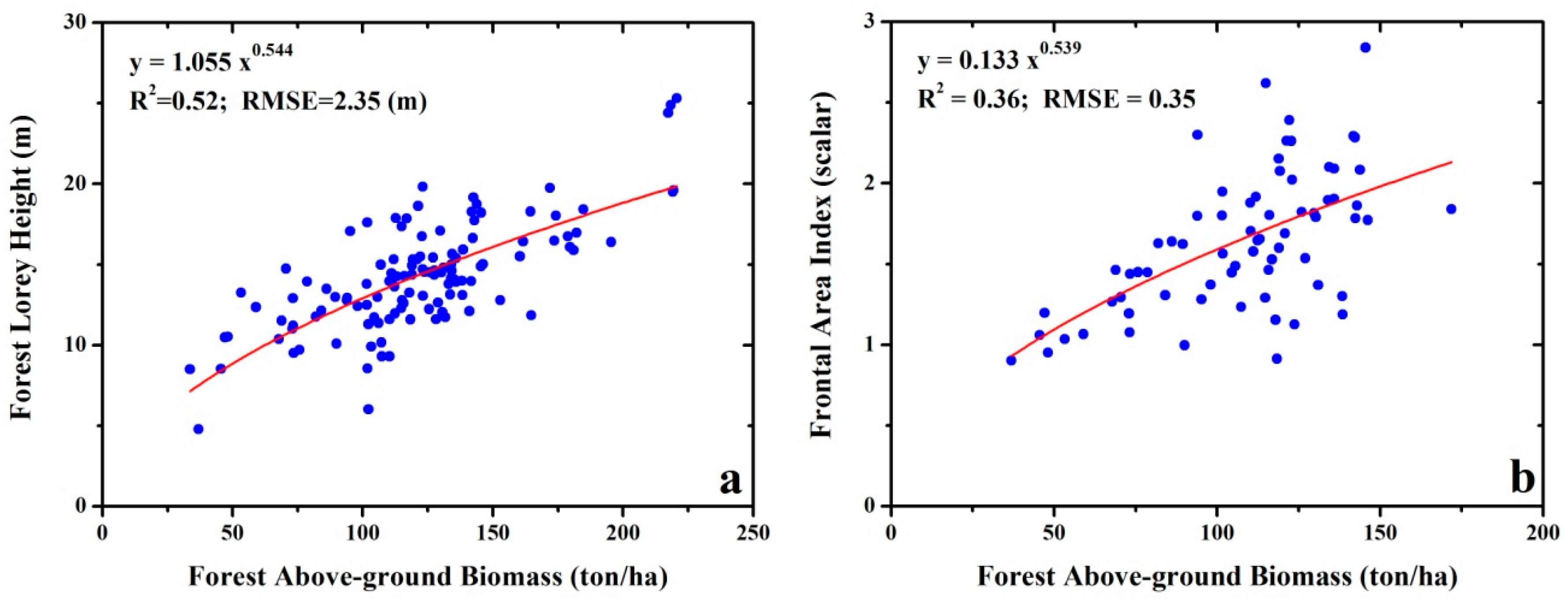
4.2. Parameterization of the SEBS

A polynomial was fitted for forest Lorey’s height (Y_L) versus forest AGB (X) based on both DBH and tree height measurements from 119 plots (out of the total 133 plots). The FAI (Y_FAI) versus forest AGB was based on tree height, and the FBH and crown width measurements from 70 plots (Figure 2).

For the Lorey’s height (Y_L), the fitting regression was, as follows:

$$Y_L=1.055\times X^{0.544}$$

(23)

where R² = 0.52 and RMSE = 2.35 meters (m).

For the FAI (Y_FAI), the fitting regression was, as follows:

$$Y_{FAI}=0.133\times X^{0.539}$$

(24)

with R² = 0.36 and RMSE = 0.35 (scalar).

The interannual forest Lorey’s height and the FAI parameters were derived from Equations (23)–(24), and the corresponding forest AGB dynamics were estimated using the Biome-BGC model calibrated using the MOD_17 model. Through the use of Equations (14)–(21) and the eight-day GLASS LAI products, the corresponding eight-day d and z_0m were derived using the SD00 model (the statistics for the interannual forest Lorey’s height, d and z_0m are shown in Table 2). The retrievals were further applied in order to estimate eight-day z_0h values using the kB⁻¹ model.

Figure 2. The fitting regression of forest Lorey’s height (a) and the frontal area index (FAI) (b) against the forest aboveground biomass (AGB) based on measurements.

Figure 2. The fitting regression of forest Lorey’s height (a) and the frontal area index (FAI) (b) against the forest aboveground biomass (AGB) based on measurements.

Table 2. Statistics for the interannual forest Lorey’s heights (h_L) (unit: meter), d (d_R: value range; d_M: mean value) (unit: meter), and z_0m (z_0m/R: value range; z_0m/M: mean value) (unit: meter) from 2000 to 2012 at the EC site.

Year	hL	dR	dM	z0m/R	z0m/M
2000	13.39	6.52–7.62	6.84	1.32–1.46	1.36
2001	13.62	7.28–10.51	8.50	0.72–1.48	1.19
2002	13.96	7.48–11.10	9.07	0.65–1.49	1.13
2003	14.30	7.69–11.39	9.25	0.67–1.51	1.16
2004	14.58	7.86–11.41	9.36	0.73–1.53	1.20
2005	14.87	8.04–11.09	9.92	0.66–1.55	1.13
2006	15.02	8.12–12.05	10.06	0.68–1.55	1.12
2007	15.24	8.25–12.35	10.22	0.66–1.57	1.14
2008	15.44	8.38–12.49	10.32	0.68–1.58	1.16
2009	15.55	8.44–12.55	10.19	0.69–1.58	1.21
2010	15.72	7.79–9.18	8.22	0.71–1.61	1.48
2011	15.90	8.65–12.81	10.44	0.71–1.60	1.22
2012	16.14	8.80–13.14	10.90	0.69–1.62	1.17

Table 2. Statistics for the interannual forest Lorey’s heights (h_L) (unit: meter), d (d_R: value range; d_M: mean value) (unit: meter), and z_0m (z_0m/R: value range; z_0m/M: mean value) (unit: meter) from 2000 to 2012 at the EC site.

Year	hL	dR	dM	z0m/R	z0m/M
2000	13.39	6.52–7.62	6.84	1.32–1.46	1.36
2001	13.62	7.28–10.51	8.50	0.72–1.48	1.19
2002	13.96	7.48–11.10	9.07	0.65–1.49	1.13
2003	14.30	7.69–11.39	9.25	0.67–1.51	1.16
2004	14.58	7.86–11.41	9.36	0.73–1.53	1.20
2005	14.87	8.04–11.09	9.92	0.66–1.55	1.13
2006	15.02	8.12–12.05	10.06	0.68–1.55	1.12
2007	15.24	8.25–12.35	10.22	0.66–1.57	1.14
2008	15.44	8.38–12.49	10.32	0.68–1.58	1.16
2009	15.55	8.44–12.55	10.19	0.69–1.58	1.21
2010	15.72	7.79–9.18	8.22	0.71–1.61	1.48
2011	15.90	8.65–12.81	10.44	0.71–1.60	1.22
2012	16.14	8.80–13.14	10.90	0.69–1.62	1.17

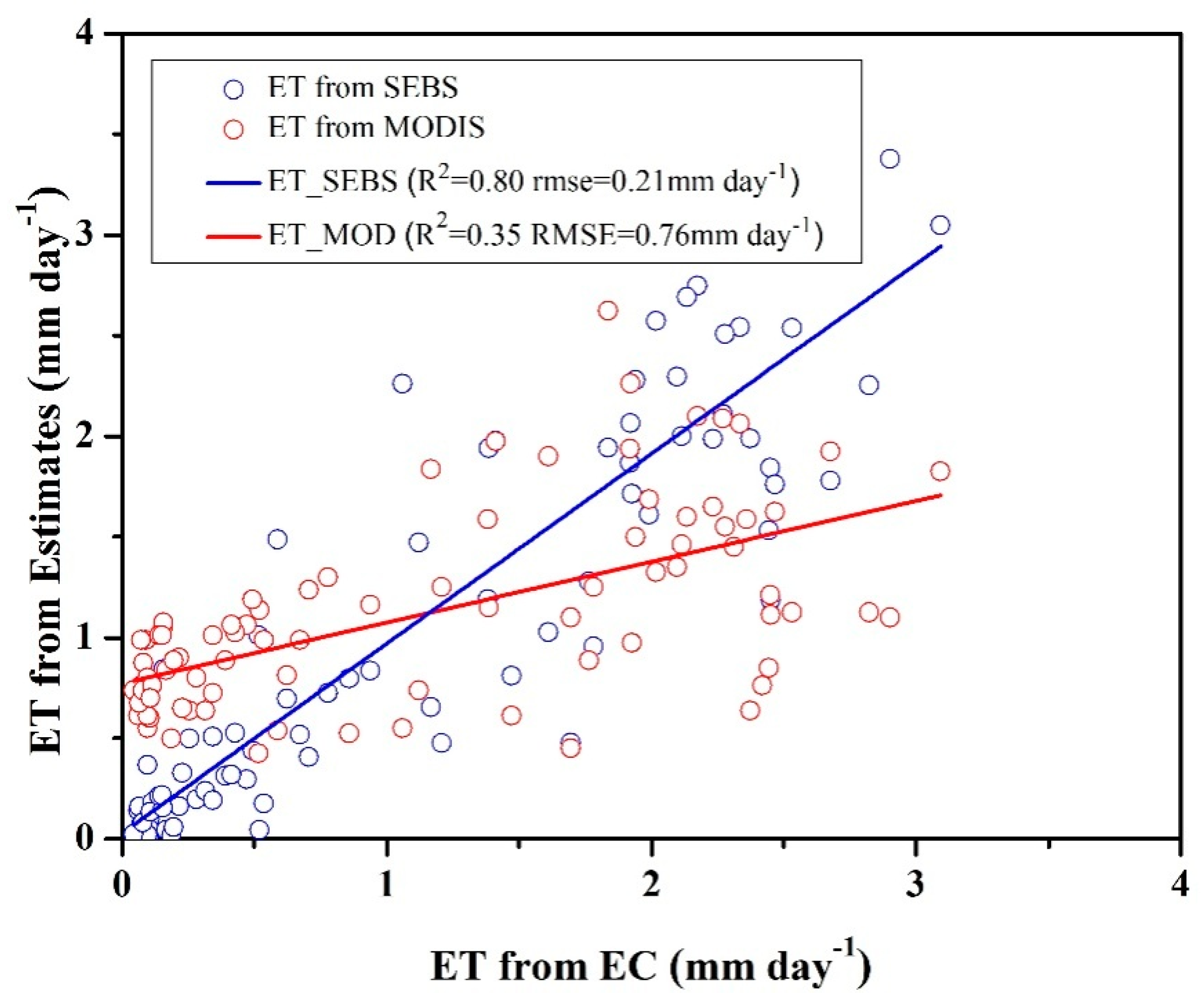
4.3. A comparison of ET Estimates between EC Measurements, the SEBS Simulations, and MODIS MOD16 Products

By incorporating original eight-day MODIS products (NDVI, LST), eight-day GLASS Albedo products, and downscaled WRF estimates (air temperature, wind speed, air and vapor pressure, and downwelling shortwave and long-wave radiations), the parameterized SEBS was employed for simulating eight-day ET from 2000 to 2012. Comparisons amongst the eight-day average ET estimates (a total of 86 samples) during 2010 and 2011 from EC, SEBS, and MODIS products are provided in Figure 3 and Figure 4.

Figure 3. A comparison of two-year, eight-day average evapotranspiration (ETs) betweenthe Surface Energy Balance System (SEBS) simulations and eddy covariance (EC) measurements.

Figure 3. A comparison of two-year, eight-day average evapotranspiration (ETs) betweenthe Surface Energy Balance System (SEBS) simulations and eddy covariance (EC) measurements.

As compared to the two-year EC measurements, the parameterized SEBS generated a reliable eight-day average ET with R² = 0.80 and RMSE = 0.21 mm·day⁻¹. The MOD16-ET biased the simulations, with R² = 0.35 and RMSE = 0.76 mm·day⁻¹. The SEBS slightly underestimated ET during the forest growing seasons (summer and autumn) during 2010 but overestimated ET for the growing seasons during 2011. As is clear from the results, the MOD16-ET significantly underestimated ET for the growing seasons but significantly overestimated ET during the spring seasons when the SEBS matched EC measurements.

Figure 4. A plot of the eight-day average SEBS simulated ET versus EC measurements.

Figure 4. A plot of the eight-day average SEBS simulated ET versus EC measurements.

4.4. Interannual ET Simulations Using the SEBS

Interannual ET dynamics (unit: mm·year⁻¹) estimated by the SEBS model over the QM forest from 2000 to 2012 are provided in Figure 5. Due to diverse environmental conditions (various meteorological and forest stand conditions) during the simulation period, the figure shows the regional distribution of interannual forest ET over a wide range. In all of the maps, due to the cold and arid conditions of the QM forest, the estimated forest ET is generally lower than 400 mm·year⁻¹. In general, forest ETs located in the northern portion are lower than those in the southern portion.

Figure 5. The interannual dynamics of forest ET simulated by the SEBS over the QMs from 2000 to 2012.

Figure 5. The interannual dynamics of forest ET simulated by the SEBS over the QMs from 2000 to 2012.

Table 3. The statistics for interannual simulated forest ETs and precipitation (unit: mm·year⁻¹) downscaled from WRF estimates over the QMs from 2000 to 2012.

Year	ETMean	ETMin	ETMax	ETsd	ETSum	P	ETMean/P(%)
2000	244	136	1016	80	190,426	454	53.74
2001	281	165	1008	76	219,356	344	81.77
2002	299	166	1025	79	233,380	453	66.02
2003	317	194	985	77	247,049	279	113.59
2004	271	158	1075	82	211,567	386	70.21
2005	290	165	949	62	225,890	454	63.77
2006	248	143	1242	97	193,126	509	48.65
2007	277	165	1150	80	216,346	671	41.34
2008	255	136	1051	82	198,537	481	52.97
2009	201	124	882	69	156,904	512	39.33
2010	222	131	969	75	173,053	482	46.05
2011	236	137	1024	79	184,386	550	42.99
2012	290	175	1015	75	225,943	499	58.11

Table 3. The statistics for interannual simulated forest ETs and precipitation (unit: mm·year⁻¹) downscaled from WRF estimates over the QMs from 2000 to 2012.

Year	ETMean	ETMin	ETMax	ETsd	ETSum	P	ETMean/P(%)
2000	244	136	1016	80	190,426	454	53.74
2001	281	165	1008	76	219,356	344	81.77
2002	299	166	1025	79	233,380	453	66.02
2003	317	194	985	77	247,049	279	113.59
2004	271	158	1075	82	211,567	386	70.21
2005	290	165	949	62	225,890	454	63.77
2006	248	143	1242	97	193,126	509	48.65
2007	277	165	1150	80	216,346	671	41.34
2008	255	136	1051	82	198,537	481	52.97
2009	201	124	882	69	156,904	512	39.33
2010	222	131	969	75	173,053	482	46.05
2011	236	137	1024	79	184,386	550	42.99
2012	290	175	1015	75	225,943	499	58.11

Correspondingly, the interannual statistics of ET (including average, minimum, maximum, stand deviation, and total amount), precipitation (downscaled from the WRF result), and ET/precipitation in the forested areas are provided in Table 3. In total, the statistics calculated from the 780 forest pixels (1 km resolution) also represented the diversity of the estimates. The table indicates that the highest annual average of forest ET (317 mm·year⁻¹) occurred during 2003 and the lowest (201 mm·year⁻¹) occurred during 2009. Interestingly, the highest ratio of annual ET/precipitation was also determined during 2003 while the lowest was found for 2009. The ratio in 2003 was higher than one, implying that forest growth during 2003 was largely supported by soil moisture.

5. Discussion

The parameters d and z_0m have been used in ET models that include MOS theory, such as the SEBS model. Although our sensitivity analysis indicated that errors within the SEBS led to estimated H values with deviations (± 25%) of z_0m that were smaller than those for LST and air temperature, a 50% deviation in the parameterization of z_0m, as well as forest height, can generate errors of more than 40% for the H estimation. The result is consistent with those presented by van der Kwast et al. [50], Zhou et al. [75], and Ma et al. [79]. In particular, according to the study of Zhou et al. [71], the annual maximum effect of the roughness length dynamic on sensible heat flux was 33.80% and 18.11% for the Qianyanzhou (with a 11–12 meter high artificial needle forest) and Changbai Mountains (with a 26 meter high natural mixed forest) experimental stations, respectively.

If canopy height information is not available for z_0m parameterization within the SEBS, it can be retrieved using the empirical equation that involves NDVI values (NDVIs of fully vegetated and bare soil), as well as maximum and minimum canopy heights. Some sensitivity analyses [38,49] for maximum height have indicated the importance of this parameter through replacement with measured values. This type of empirical method may be suitable for low canopies with short height ranges. However, due to the saturation of spectral signals, the NDVI in forests cannot represent canopy height variations, so canopy heights, especially for long-term heterogeneous forest parameterization, will generally be underestimated.

Additional studies [43,44,47] have indicated that vegetation vertical parameters (i.e., the height and FAI) are critical for estimates of d and z_0m obtained via remote sensing-based roughness models [42,43,44]. However, few studies have focused on the long term parameterization scheme of d and z_0m while considering the variation of vertical vegetation information over time. Vegetation height is commonly derived from vegetation indexes (i.e., NDVI and LAI) using optical remote sensing data that may be suitable for low vegetation (for example, pastures, crops, shrubs, etc.) [80,81] or that can be derived from active remote sensing (i.e., Synthetic Aperture Radar (SAR) and Light Detection and Ranging (LiDAR)) data sensitive to forest vertical structure [82,83]. Nevertheless, these methods are not possible for growing forests. On the one hand, vegetation indexes in the QMs represent a mixture of the top canopy and the understory in forest gaps. On the other hand, the local extremely complicated terrain condition hinders SAR data applicability, and expensive single-pass airborne LiDAR data obtained by WATER can only derive vegetation height over a certain period and for a certain area. Therefore, at present, remote sensing data cannot provide reliable forest vertical dynamic information for this study area.

In an earlier study [47], we reported that the SD00 model outperformed other aerodynamic roughness models. Here, dynamic forest vertical information for height and the FAI were obtained from field calibrated regression models and interannual forest AGB variations in order to drive the SD model. Instead of the arithmetical mean height, the Lorey’s height was derived due to the fact that it is a better expression for forest stand status, as well as for d and z_0m [44,47]. Although the R² values (0.52 and 0.36) of both fittings were not high, the RMSEs (2.35 m and 0.35 were relatively low. Based on the high heterogeneity of local forests under various stand conditions (topography, tree density, height, FBH, age, AGB level, overlapping canopies, etc.), regression relationships (forest Lorey’s height versus forest AGB and FAI versus forest AGB) established on the basis of forest measurements were reasonable. However, due to natural disturbance, as well as the self-adaption, in forests, Lorey’s height and the FAI are apt to defy the regressions. For example, as a result of self-thinning adaption, matured or over-matured forests would definitely change SD (trees·ha⁻¹) so that ecosystem balance is maintained, causing an increase in forest height and a decrease in forest AGB. As understood, forest AGB levels should obey a parabolic relationship between forest AGB and forest age. In this study, regression models based on measurements without forest age information would be biased, because, in practice, different forest heights exist in stands that have a similar forest AGB level but various stand densities. Additional studies should take forest stand age and forest SD into account in their analyses. Alternatively, continuous national forest inventories using a five-year interval and upcoming active spaceborne remote sensing (i.e., the Chinese high-resolution satellite constellation with SAR and LiDAR sensors on board) with the ability to derive multi-temporal forest vertical parameters could also be helpful for calibrating bias for local forest vertical information.

According to the statistics of the dynamics of interannual forest ET and meteorological data obtained from the downscaled WRF, local forest ET is the most sensitive to a vapor pressure deficit (VPD), then temperature, precipitation, and downwelling short wave radiation (DSR). VPD, temperature, and precipitation yielded negative correlation to forest ET while DSR yielded a positive correlation. For example, for the 13 years analyzed, the highest forest ET occurred during 2003, the year with the second lowest VPD, the low temperature, the least amount of precipitation, and a sufficient DSR; while the lowest forest ET was determined for 2009 that had the second highest VPD and temperature, moderate precipitation, and a low DSR. As shown in Table 3, the ratio of ET to precipitation during 2003 was higher than one, implying that during this driest year soil moisture contributes the most positive “green water” (the water mainly used by the ecosystem itself [84]) to the forest ecosystem.

In forested areas with altitudes from 2600 to 3300 m, surface soil with a field water capacity of more than 50% [85] is largely covered by moss and litter with a very high porosity and a low bulk density, resulting in a high evapotranspiration rate and hydraulic conductivity. Thus, the Picea crassifolia forest has the greatest potential water retention capacity [86]. The water storage capacity of the soil in this area was determined to be 39.14%, and 37.38% higher within the Picea crassifolia forest than in Sabina przewalsk forest and shrubs, respectively, at a similar soil depth [87]. The higher soil water content may result in a higher plant transpiration rate, as indicated in the study of Chang et al., [85] who stated that the relationship between sap flow and soil moisture content was a logistic function.

Overall, the performance of the SEBS in this study is promising and the results are comparable to those of other studies [49,88,89,90]. For example, based on the input data retrieved from multiple sensors onboard NASA Earth Observing Satellites (EOS) and the AVHRR sensor, as well as model-derived surface pressure and winds from NASA’s Global Modeling and Assimilation Office, daily global ETs were estimated by Vinukollu et al. [88] using the SEBS, the Penman-Monteith (P-M), and the Priestley-Taylor (P-T) models for the years 2003–2006. Evaluations using an inferred ET estimate based on a long-term water balance residual of precipitation minus runoff for large river basins and on a global scale yielded a good correlation (the mean correlation—the Kendall’s τ from 0.72 to 0.79). The study of Vinukollu et al. [89], that reported long-term global ET estimations for 1984–2007 using the SEBS, P-M, and P-T models, indicated a downward trend for global ET after 1998. In our study, we also found a similar downward trend within the study area since 2000 due to a warmer and wetter climate. Based on MODIS products, the results presented here are similar to those reported by Byun et al. [49] who applied the SEBS within a forest site located in the middle of the Korean peninsula, with R² = 0.80 (for this case) versus 0.88 and with RMSE = 0.21 mm·day⁻¹ (for this case) versus 0.22 mm·day⁻¹. Ma et al. [91] incorporated the TM using diverse compositions of forcing and in situ meteorological data in order to estimate daily ETs using the SEBS over the Coleambally Irrigation Area, located in the southwestern portion of New South Wales, Australia. Their results yielded a higher R² (up to 0.95) than we report here that can be ascribed to high-resolution remotely sensed data and other high-resolution and accurate inputs for homogenous irrigated croplands. However, the RMSE of their results was up to 0.74 mm·day⁻¹, larger than those we report here. The result can be explained by understanding that due to abundant irrigation daily ETs over croplands are much larger than daily forest ETs for the QMs. In a similar manner, when applying Chinese satellite HJ-1images (with a 30 m visible, 150m near-infrared, and 300 m thermal infrared bands), the same WRF estimates as those used in this study, the SEBS generated comparable results for irrigated cropland sites located within the middle reaches of the HRB [92] (with R² = 0.79 and RMSE = 0.58 mm·day⁻¹ at the vegetable site; R² = 0.81 and RMSE = 1.29 mm·day⁻¹ at the maize site; and R² = 0.86 and RMSE = 1.25 mm·day⁻¹ at the orchard site). However, due to the heterogeneity of the vegetation, the performance of the SEBS was reduced (with R² = 0.53 and RMSE = 0.67 mm·day⁻¹) at the wetland site.

In general, the SEBS model could perform well in areas with low vegetation or bare soil [38]. Nevertheless, the SEBS also showed inferiority in forested areas, especially for heterogeneous forests [93,94]. As Weligepolage et al. [95] indicated, correction terms that adjust the effects of the roughness sub-layer could contribute to improve the SEBS’s performance in areas containing complex vegetation structural scenarios [72]. Further improvement of ET can be obtained using more accurate meteorological inputs, although in our study meteorological inputs have been verified to be reliable. Some improvements of wind speed and downwelling long-wave radiation estimates are still possible [62]. As indicated by the HiWATER team, other improvements for long-term MODIS LST inputs can also be expected [96]. Using unreliable meteorological inputs and MODIS LST products for the SEBS would result in deterioration for the agreement of both H and λE, and, thus, ET and EC measurements [97,98].

The SEBS model has been proven to be reliable for multi-scale ET estimations. However, only a few studies have focused on short-term simulations within forests [65,70]. Due to complicated heat transfer mechanisms within forests and their surroundings, the SEBS cannot consistently capture the ET process. For cold and arid forests with high heterogeneity, such as the ones analyzed in this study, climate and environmental factors were found to enhance the complexity of the ET process. For example, melting snow within the canopy and underground possibly has a large impact on the ET process. Some sharply increasing daily ET values were determined for EC measurements during the late spring and early summer, indicating that this is the case (Figure 3). Further improvements should be expected if soil moisture simulations and snow melt monitoring modules are embedded into the SEBS algorithm [99]. Moreover, the appropriate parameterization of z_0h is also critical for improving the behavior of the SEBS [38,89]. Such additions could make the SEBS more applicable for multiple biomes and various climate and environmental conditions.

6. Conclusions

For this study, we conducted a sensitivity analysis. The z_0m, as well as forest height, turned out to be one of the most important factors for parameterizing the SEBS, whose 50% deviations could generate errors of more than 40% for the SEBS derived sensible heat fluxes. As the forest structural dynamic information (height, FBH, crown width, and LAI) largely affect the temporal changes in z_0m, it is necessary to apply the multi-disciplinary techniques to develop the effective parameterization of z_0m.

Here, we propose a time-series parameterization scheme (for the years 2000 to 2012) for two critical parameters (d and z_0m) using MOS theory, which is the basic mechanism for the SEBS. We calibrated two parameters (the forest height and FAI) of the SD00 model against forest measurements using regression models. The two regression equations were linked to interannual forest AGB dynamics derived from 2009 forest AGB basis maps and interannual forest AGB increments obtained from the synergistic simulations of two ecological models. By combining GLASS LAI products, forest height, and FAI dynamics, d and z_0m were derived using the SD00 model. Afterward, d and z_0m were further employed in order to derive z_0h using the kB⁻¹ model. These three parameters were used to parameterize the SEBS from 2000 to 2012. With the incorporation of original MODIS products (NDVI and LST), GLASS LAI, Albedo products, and downscaled WRF estimates, the parameterized SEBS was used to simulate eight-day forest ET over the QMs. As compared to MODIS MOD16 ET products (eight-day average) at the site (the nearest pixel), the SEBS estimates (eight-day average) were much better and agreed well with EC measurements, with the exception of the growing seasons for which the SEBS underestimated forest ET during 2010 and overestimated ET during 2011.

The dynamic parameterization scheme employed in this study is more realistic than that obtained by assuming “static” conditions based on constant values for d, z_0m, and z_0h. The spatial distribution of forest ET estimates provides valuable information for the sustainable management of forest and water resources, which are extremely important to the QMs and the entire HRB river basin. Runoff generated from mountainous regions is recognized as the main water source for the HRB. The local forests are important for flood control, runoff regulation, and soil erosion control, and, thus, contribute to hydrological service at the basin scale. The interannual forest ETs, as estimated here, showed a downward trend that was largely caused by a local climate trend of warm dryness to warm wetness [100]. Moreover, the current forest belt may shift upward in response to warm wetness, and the grassland (or shrubland) above an elevation of 3300 m may convert to a forest on shady slopes [86]. Rigorous local forest protection measures, including the expansion of grazing prohibition areas and the conversion of grasslands to secondary Picea crassifolia forests, that have been implemented within the Qilian Mountains since the 1980s could have caused decreased runoff but may also have expanded the water retention capacity of this mountain ecosystem.

References

1. Bouwer, L.M.; Biggs, T.W.; Aerts, J. Estimates of spatial variation in evaporation using satellite-derived surface temperature and a water balance model. Hydrol. Process. 2008, 22, 670–682. [Google Scholar] [CrossRef]
2. Fisher, J.B.; Tu, K.P.; Baldocchi, D.D. Global estimates of the land-atmosphere water flux based on monthly AVHRR and ISLSCP-II data, validated at 16 FLUXNET sites. Remote Sens. Environ. 2008, 112, 901–919. [Google Scholar] [CrossRef]
3. Jung, M.; Reichstein, M.; Ciais, P.; Seneviratne, S.I.; Sheffield, J.; Goulden, M.L.; Bonan, G.; Cescatti, A.; Chen, J.; Jeu, R.D.; et al. Recent decline in the global land evapotranspiration trend due to limited moisture supply. Nature 2010, 467, 951–954. [Google Scholar] [CrossRef] [PubMed]
4. Liu, Y.; Zhou, Y.; Ju, W.; Chen, J.; Wang, S.; He, H.; Wang, H.; Guan, D.; Zhao, F.; Li, Y.; et al. Evapotranspiration and water yield over China’s landmass from 2000 to 2010. Hydrol. Earth Syst. Sci. 2013, 17, 4957–4980. [Google Scholar] [CrossRef]
5. Oki, T.; Kanae, S. Global hydrological cycles and world water resources. Science 2006, 313, 1068–1072. [Google Scholar] [CrossRef] [PubMed]
6. Trenberth, K.E.; Smith, L.; Qian, T.; Dai, A.; Fasullo, J. Estimates of the global water budget and its annual cycle using observational and model data. J. Hydrometeorol. 2007, 8, 758–769. [Google Scholar] [CrossRef]
7. Trenberth, K.E.; Fasullo, J.T.; Kiehl, J. Earth’s global energy budget. Am. Meteorol. Soc. 2009, 90, 311–323. [Google Scholar] [CrossRef]
8. Molders, N.; Rabe, A. Numerical investigations on the influence of subgrid-scale surface heterogeneity on evapotranspiration and cloud processes. J. Appl. Meteorol. 1996, 35, 782–795. [Google Scholar] [CrossRef]
9. Koster, R.D.; Dirmeyer, P.A.; Guo, Z.C.; Bonan, G.; Chan, E.; Cox, P.; Gordon, C.T.; Kanae, S.; Kowalczyk, E.; Lawrence, D.; et al. Regions of strong coupling between soil moisture and precipitation. Science 2004, 305, 1138–1140. [Google Scholar] [CrossRef] [PubMed]
10. Spracklen, D.V.; Arnold, S.R.; Taylor, C.M. Observations of increased tropical rainfall preceded by air passage over forests. Nature 2012, 489, 282–285. [Google Scholar] [CrossRef] [PubMed]
11. Githui, F.; Selle, B.; Thayalakumaran, T. Recharge estimation using remotely sensed evapotranspiration in an irrigated catchment in southeast Australia. Hydrol. Process. 2012, 26, 1379–1389. [Google Scholar] [CrossRef]
12. Campos, G.E.P.; Moran, M.S.; Huete, A.; Zhang, Y.G.; Bresloff, C.; Huxman, T.E.; Eamus, D.; Bosch, D.D.; Buda, A.R.; Gunter, S.A.; et al. Ecosystem resilience despite large-scale altered hydroclimatic conditions. Nature 2013, 494, 349–352. [Google Scholar] [CrossRef] [PubMed]
13. Keenan, T.F.; Hollinger, D.Y.; Bohrer, G.; Dragoni, D.; Munger, J.W.; Schmid, H.P.; Richardson, A.D. Increase in forest water-use efficiency as atmospheric carbon dioxide concentrations rise. Nature 2013, 499, 324–327. [Google Scholar] [CrossRef] [PubMed]
14. Wang, S.S.; Yang, Y.; Trishchenko, A.P.; Barr, A.G.; Black, T.A.; McCaughey, H. Modelling the response of canopy stomatal conductance to humidity. J. Hydrometeorol. 2009, 10, 521–532. [Google Scholar] [CrossRef]
15. Wang, S.; Yang, Y.; Luo, Y.; Rivera, A. Spatial and seasonal variations in evapotranspiration over Canada’s landmass. Hydrol. Earth Syst. Sci. 2013, 17, 3561–3575. [Google Scholar] [CrossRef]
16. Yuan, W.P.; Liu, S.G.; Yu, G.R.; Bonnefond, J.M.; Chen, J.Q.; Davis, K.; Desai, A.R.; Goldstein, A.H.; Gianelle, D.; Rossi, F.; et al. Global estimates of evapotranspiration and gross primary production based on MODIS and global meteorology data. Remote Sens. Environ. 2010, 114, 1416–1431. [Google Scholar] [CrossRef]
17. Fisher, J.B.; Whittaker, R.J.; Malhi, Y. ET come home: Potential evapotranspiration in geographical ecology. Glob. Ecol. Biogeogr. 2011, 20, 1–18. [Google Scholar] [CrossRef]
18. Zeng, Z.Z.; Piao, S.L.; Lin, X.; Yin, G.D.; Peng, S.S.; Ciais, P.; Myneni, R.B. Global evapotranspiration over the past three decades: Estimation based on the water balance equation combined with empirical models. Environ. Res. Lett. 2012. [Google Scholar] [CrossRef]
19. Jackson, R.B.; Carpenter, S.R.; Dahm, C.N.; McKnight, D.M.; Naiman, R.J.; Postel, S.L.; Running, S.W. Water in a changing world. Ecol. Appl. 2001, 11, 1027–1045. [Google Scholar] [CrossRef]
20. Li, Z.L.; Tang, R.L.; Wan, Z.M.; Bi, Y.Y.; Zhou, C.H.; Tang, B.H.; Yan, G.J.; Zhang, C.Y. A review of current methodologies for regional evapotranspiration estimation from remotely sensed data. Sensors 2009, 9, 3801–3853. [Google Scholar] [CrossRef] [PubMed]
21. Wang, K.C.; Dickinson, R.E. A review of global terrestrial evapotranspiration: Observation, modeling, climatology, and climatic variability. Rev. Geohys. 2012. [Google Scholar] [CrossRef]
22. Kustas, W.P.; Norman, J.M. Use of remote sensing for evapotranspiration monitoring over land surfaces. Hydrol. Sci. J. 1996, 41, 495–516. [Google Scholar] [CrossRef]
23. Su, Z. The surface energy balance system (SEBS) for estimation of turbulent heat fluxes. Hydrol. Earth Syst. Sci. 2002, 6, 85–99. [Google Scholar] [CrossRef]
24. Ju, W.M.; Gao, P.; Wang, J.; Zhou, Y.L.; Zhang, X.H. Combining an ecological model with remote sensing and GIS techniques to monitor soil water content of croplands with a monsoon climate. Agric. Water Manag. 2010, 97, 1221–1231. [Google Scholar] [CrossRef]
25. Yang, Y.T.; Shang, S.H.; Jiang, L. Remote sensing temporal and spatial patterns of evapotranspiration and the responses to water management in a large irrigation district of North China. Agric. For. Meteorol. 2012, 164, 112–122. [Google Scholar] [CrossRef]
26. Ryu, Y.; Baldocchi, D.D.; Kobayashi, H.; van Ingen, C.; Li, J.; Black, T.A.; Beringer, J.; van Gorsel, E.; Knohl, A.; Law, B.E.; et al. Integration of MODIS land and atmosphere products with a coupled-process model to estimate gross primary productivity and evapotranspiration from 1 km to global scales. Glob. Biogeochem. Cycles 2011. [Google Scholar] [CrossRef]
27. Bastiaanssen, W.G.M.; Menenti, M.; Feddes, R.A.; Holtslag, A.A.M. A remote sensing surface energy balance algorithm for land (SEBAL). 1. Formulation. J. Hydrol. 1998, 212–213, 198–212. [Google Scholar] [CrossRef]
28. Miralles, D.G.; Holmes, T.R.H.; de Jeu, R.A.M.; Gash, J.H.; Meesters, A.G.C.A.; Dolman, A.J. Global land-surface evaporation estimated from satellite-based observations. Hydrol. Earth Syst. Sci. 2011, 15, 453–469. [Google Scholar] [CrossRef]
29. Anderson, R.G.; Jin, Y.F.; Goulden, M.L. Assessing regional evapotranspiration and water balance across a Mediterranean montane climate gradient. Agric. For. Meteorol. 2012, 166, 10–22. [Google Scholar] [CrossRef]
30. Wang, K.C.; Liang, S.L. An improved method for estimating global evapotranspiration based on satellite determination of surface net radiation, vegetation index, temperature, and soil moisture. J. Hydrometeorol. 2008, 9, 712–727. [Google Scholar] [CrossRef]
31. Mu, Q.; Heinsch, F.A.; Zhao, M.; Running, S.W. Development of a global evapotranspiration algorithm based on MODIS and global meteorology data. Remote Sens. Environ. 2007, 111, 519–536. [Google Scholar] [CrossRef]
32. Zhang, K.; Kimball, J.S.; Nemani, R.R.; Running, S.W. A continuous satellite-derived global record of land surface evapotranspiration from 1983 to 2006. Water Resour. Res. 2010. [Google Scholar] [CrossRef]
33. Rodell, M.; McWilliams, E.B.; Famiglietti, J.S.; Beaudoing, H.K.; Nigro, J. Estimating evapotranspiration using an observation based terrestrial water budget. Hydrol. Process. 2011, 25, 4082–4092. [Google Scholar] [CrossRef]
34. Sahoo, A.K.; Pan, M.; Troy, T.J.; Vinukollu, R.K.; Sheffield, J.; Wood, E.F. Reconciling the global terrestrial water budget using satellite remote sensing. Remote Sens. Environ. 2011, 115, 1850–1865. [Google Scholar] [CrossRef]
35. Su, Z.B.; Zhang, T.; Ma, Y.M.; Jia, L.; Wen, J. Energy and water cycle over the Tibetan Plateau: Surface energy balance and turbulent heat fluxes. Adv. Earth Sci. 2006, 21, 1224–1236. [Google Scholar]
36. Fernández-Prieto, D.; van Oevelen, P.; Su, Z.; Wagner, W. Advances in Earth observation for water cycle science. Hydrol. Earth Syst. Sci. 2012, 16, 543–549. [Google Scholar] [CrossRef]
37. Jia, Z.Z.; Liu, S.M.; Xu, Z.W.; Chen, Y.Y.; Zhu, M.J. Validation of remotely sensed evapotranspiration over the Hai River Basin, China. J. Geophys. Res. 2012. [Google Scholar] [CrossRef]
38. Chen, X.L.; Su, Z.B.; Ma, Y.M.; Yang, K.; Wen, J.; Zhang, Y. An improvement of roughness height parameterization of the Surface Energy Balance System (SEBS) over the Tibetan Plateau. J. Appl. Meteorol. Climatol. 2013, 52, 607–622. [Google Scholar] [CrossRef]
39. Monin, A.S.; Obukhov, A.M. Basic laws of turbulent mixing in the ground layer of the atmosphere. Trudy Geofiz. Instit. Akad. Nauk SSSR 1954, 24, 163–187. [Google Scholar]
40. Foken, T. 50 years of the Monin-Obukhov similarity theory. Bound. Layer Meteorol. 2006, 119, 431–447. [Google Scholar] [CrossRef]
41. Choudhury, B.J.; Monteith, J.L. A four-layer model for the heat budget of homogeneous land surfaces. Q. J. R. Meteorol. Soc. 1988, 114, 373–398. [Google Scholar] [CrossRef]
42. Raupach, M.R. Simplified expressions for vegetation roughness length and zero-plane displacement as a function of canopy height and area index. Bound.-Layer Meteorol. 1994, 71, 211–216. [Google Scholar] [CrossRef]
43. Schaudt, K.J.; Dickinson, R.E. An approach to deriving roughness length and zero-plane displacement height from satellite data, prototyped with BOREAS data. Agric. For. Meteorol. 2000, 104, 143–155. [Google Scholar] [CrossRef]
44. Nakai, T.; Sumida, A.; Daikoku, K.; Matsumoto, K.; van der Molen, M.K.; Kodama, Y.; Kononov, A.V.; Maximov, T.C.; Dolman, A.J.; Yabuki, H.; et al. Parameterisation of aerodynamic roughness over boreal, cool- and warm-temperate forests. Agric. For. Meteorol. 2008, 148, 1916–1925. [Google Scholar] [CrossRef]
45. Su, Z.; Schmugge, T.; Kustas, W.P.; Massman, W.J. An evaluation of two models for estimation of the roughness height for heat transfer between the land surface and the atmosphere. J. Appl. Meteorol. 2001, 40, 1933–1951. [Google Scholar] [CrossRef]
46. Yang, K.; Koike, T.; Fujii, H.; Tamagawa, K.; Hirose, N. Improvement of surface flux parametrizations with a turbulence related length. Q. J. R. Meteorol. Soc. 2002, 128, 2073–2087. [Google Scholar] [CrossRef]
47. Tian, X.; Li, Z.Y.; van der Tol, C.; Su, Z.; Li, X.; He, Q.S.; Bao, Y.F.; Chen, E.X.; Li, L.H. Estimating zero-plane displacement height and aerodynamic roughness length using synthesis of LiDAR and SPOT-5 data. Remote Sens. Environ. 2011, 115, 2330–2341. [Google Scholar] [CrossRef]
48. Gibson, L.; Münch, Z.; Engelbrecht, J. Particular uncertainties encountered inusing a pre-packaged SEBS model to derive evapotranspiration in a heteroge-neous study area in South Africa. Hydrol. Earth Syst. Sci. 2011, 15, 295–310. [Google Scholar] [CrossRef] [Green Version]
49. Byun, K.; Liaqat, U.W.; Choi, M. Dual-model approaches for evapotranspiration analyses over homo- and heterogeneous land surface conditions. Agric. For. Meteorol. 2014, 197, 169–187. [Google Scholar] [CrossRef]
50. Van der Kwast, J.; Timmermans, W.; Gieske, A.; Su, Z.B.; Oliso, A.; Jia, L.; Elbers, J.; Karssenberg, D.; de Jong, S. Evaluation of the Surface Energy Balance System (SEBS) applied to ASTER imagery with flux-measurements at the SPARC 2004 site (Barrax, Spain). Hydrol. Earth Syst. Sci. 2009, 13, 1337–1347. [Google Scholar] [CrossRef]
51. Lorey, T. Die mittlereBestandeshohe. Allg. Forst J. Ztg. 1878, 54, 149–155. [Google Scholar]
52. Tian, X.; Yan, M.; van der Tol, C.; Li, Z.Y.; Su., Z.B.; Chen, E.X.; Li, X.; Li, L.H.; Wang, X.F.; Pan, X.D.; et al. Modeling of forest above-ground biomass dynamics using multi-sourced remote sensing data and incorporated models. Remote Sens. Environ. 2015. in resubmission. [Google Scholar]
53. Tian, X.; Li, Z.Y.; Su, Z.B.; Chen, E.X.; van der Tol, C.; Li, X.; Guo, Y.; Li, L.H.; Ling, F.L. Estimating montane forest above-ground biomass in the upper reaches of the Heihe River Basin using Landsat-TM data. Int. J. Remote Sens. 2014, 35, 7339–7362. [Google Scholar] [CrossRef]
54. Li, X.; Li, X.W.; Li, Z.Y.; Ma, M.G.; Wang, J.; Xiao, Q.; Liu, Q.; Che, T.; Chen, E.X.; Yan, G.J.; et al. Watershed allied telemetry experimental research. J. Geophys. Res. 2009. [Google Scholar] [CrossRef]
55. Li, X.; Li, X.W.; Roth, K.; Menenti, M.; Wagner, W. Preface “Observing and modeling the catchment scale water cycle”. Hydrol. Earth Syst. Sci. 2011, 15, 597–601. [Google Scholar] [CrossRef]
56. Wang, W.Z.; Xu, Z.W.; Liu, S.M.; Li, X.; Ma, M.G.; Wang, J.M. The Characteristics of Heat and Water Vapor Fluxes over Different Surfaces in the Heihe River Basin. Adv. Earth Sci. 2009, 7, 714–723. (In Chinese) [Google Scholar]
57. Zhang, Z.H.; Wang, W.Z.; Ma, M.G.; Wu, Y.R.; Xu, Z.W. The processing methods of eddy covariance flux data and products in “WATER” Test. Remote Sens. Technol. Appl. 2010, 25, 788–796. (In Chinese) [Google Scholar]
58. Wang, X.F.; Ma, M.G.; Song, Y.; Tan, J.L.; Wang, H.B. Coupling of a biogeochemical model with a simultaneous heat and water model and its evaluation at an alpine meadow site. Environ. Earth Sci. 2014. [Google Scholar] [CrossRef]
59. Wang, J.Y.; Ju, K.J.; Fu, H.E.; Chang, X.X.; He, H.Y. Study on biomass of water conservation forest on north slope of Qilian mountains. J. Fujian Coll. For. 1998, 18, 319–323. (In Chinese) [Google Scholar]
60. Liston, G.E.; Elder, K. A meteorological distribution system for high-resolution terrestrial modeling (MicroMet). J. Hydrometeorol. 2006, 7, 217–234. [Google Scholar] [CrossRef]
61. Pan, X.D.; Li, X. Validation of WRF model on simulating forcing data for Heihe River Basin. Sci. Cold Arid Reg. 2011, 3, 344–357. [Google Scholar]
62. Pan, X.D.; Li, X.; Shi, X.K.; Han, X.J.; Luo, L.H.; Wang, L.X. Dynamic downscaling of near-surface air temperature at the basin scale using WRF—A case study in the Heihe River Basin, China. Front. Earth Sci. 2012, 6, 314–323. [Google Scholar] [CrossRef]
63. Liang, S.L.; Zhao, X.; Liu, S.H.; Yuan, W.P.; Cheng, X.; Xiao, Z.Q.; Zhang, X.T.; Liu, Q.; Cheng, J.; Tang, H.R.; et al. A long-term global Land surface satellite (GLASS) data-set for environmental studies. Int. J. Digit. Earth 2013, 6, 5–33. [Google Scholar] [CrossRef]
64. Generation & Application of Global Products of Essential Land Variables. Available online: http://glass-product.bnu.edu.cn (accessed on 26 July 2015).
65. Level 1 and Atomosphere Archive and Distribution System. Available online: http://ladsweb.nascom.nasa.gov (accessed on 26 July 2015).
66. ASTER Global Digital Elevation Model (GDEM). Available online: http://www.gdem.aster.ersdac.or.jp (accessed on 26 July 2015).
67. Numerical Terrdynamic Simulation Group. Available online: http://www.ntsg.umt.edu/project/mod16 (accessed on 26 July 2015).
68. Brutsaert, W. Aspect of bulk atmospheric boundary layer similarity under free-convective conditions. Rev. Geohys. 1999, 37, 439–451. [Google Scholar] [CrossRef]
69. Su, H.B.; McCabe, M.F.; Wood, E.F.; Su, Z.; Prueger, J.H. Modeling evapotranspiration during SMACEX: Comparing two approaches for local- and regional-scale prediction. J. Hydrometeorol. 2005, 6, 910–922. [Google Scholar] [CrossRef]
70. Pan, M.; Wood, E.F.; Wojcik, R.; McCabe, M.F. Estimation of regional terrestrial water cycle using multi-sensor remote sensing observations and data assimilation. Remote Sens. Environ. 2008, 112, 1282–1294. [Google Scholar] [CrossRef]
71. Sobrino, J.A.; Gomez, M.; Jimenez-Munoz, C.; Olioso, A. Application of a simple algorithm to estimate daily evapotranspiration from NOAA-AVHRR images for the Iberian Peninsula. Remote Sens. Environ. 2007, 110, 139–148. [Google Scholar] [CrossRef]
72. Chirouze, J.; Boulet, G.; Jarlan, L.; Fieuzal, R.; Rodriguez, J.C.; Ezzahar, J.; Raki, S.E.; Bigeard, G.; Merlin, O.; Garatuza-Payan, J.; et al. Intercomparison of four remote-sensing-based energy balance methods to retrieve surface evapotranspiration and water stress of irrigated fields in semi-arid climate. Hydrol. Earth Syst. Sci. 2014, 18, 1165–1188. [Google Scholar] [CrossRef] [Green Version]
73. Ma, W.Q.; Ma, Y.M.; Shikawa, H. Evaluation of the SEBS for upscaling the evapotranspiration based on in-situ observations over the Tibetan Plateau. Atmos. Res. 2014, 138, 91–97. [Google Scholar] [CrossRef]
74. Pardo, N.; Sanchez, M.L.; Timmermans, J.; Su, Z.B.; Perez, I.A.; Garcia, M.A. SEBS validation in a Spanish rotating crop. Agric. For. Meteorol. 2014, 195, 132–142. [Google Scholar] [CrossRef]
75. Zhou, Y.L.; Sun, X.M.; Zhu, Z.L.; Zhang, R.H.; Tian, J.; Liu, Y.F.; Guan, D.X.; Yuan, G.F. Surface roughness length dynamic over several different surfaces and its effects on modeling fluxes. Sci. China Ser. D-Earth Sci. 2006, 49, 262–272. [Google Scholar] [CrossRef]
76. Ershadi, A.; McCabe, M.F.; Evans, J.P.; Chaney, N.W.; Wood, E.F. Multi-site evaluation of terrestrial evaporation models using FLUXNET data. Agric. For. Meteorol. 2014, 187, 46–61. [Google Scholar] [CrossRef]
77. Zhuo, G.; La, B.; Pubu, C.; Luo, B. Study on daily surface evapotranspiration with SEBS in Tibet Autonomous Region. J. Geogr. Sci. 2014, 24, 113–128. [Google Scholar] [CrossRef]
78. Massman, W. An analytical one-dimensional model of momentum transferby vegetation of arbitrary structure. Bound.-Layer Meteorol. 1997, 83, 407–421. [Google Scholar] [CrossRef]
79. Ma, W.Q.; Ma, Y.M.; Hu, Z.Y.; Su, Z.B.; Wang, J.M.; Ishikawa, H. Estimating surface fluxes over middle and upper streams of the Heihe River Basin with ASTER imagery. Hydrol. Earth Syst. Sci. 2011, 15, 1403–1413. [Google Scholar] [CrossRef]
80. Ramsey, E.W.; Jensen, J.R. Remote sensing of mangrove wetlands: Relating canopy spectra to site-specific data. Photogramm. Eng. Remote Sens. 1996, 62, 939–948. [Google Scholar]
81. Papadavid, G.; Fasoula, D.; Hadjimitsis, M.; Perdikou, P.S.; Hadjimitsis, D.G. Image based remote sensing method for modeling black-eyed beans (Vignaunguiculata) Leaf Area Index (LAI) and Crop Height (CH) over Cyprus. Cent. Eur. J. Geosci. 2013, 5, 1–11. [Google Scholar]
82. Kovacs, J.M.; Lu, X.X.; Flores-Verdugo, F.; Zhang, C.; de Santiago, F.F.; Jiao, X. Applications of ALOS PALSAR for monitoring biophysical parameters of a degraded black mangrove (Avicenniagerminans) forest. ISPRS J. Photogramm. Remote Sens. 2013, 82, 102–111. [Google Scholar] [CrossRef]
83. Lefsky, M.A.; Cohen, W.B.; Acker, S.A.; Parker, G.G.; Spies, T.A.; Harding, D. Lidar remote sensing of the canopy structure and biophysical properties of Douglas-fir western hemlock forests. Remote Sens. Environ. 1999, 70, 339–361. [Google Scholar] [CrossRef]
84. Falkenmark, M.; Rockström, J. The new blue and green water paradigm: Breaking new ground for water resources planning and management. J. Water Resour. Plan. Manag. 2006, 132, 129–132. [Google Scholar] [CrossRef]
85. Change, X.X.; Zhao, W.Z.; He, Z.B. Radial pattern of sap flow and response to microclimate and soil moisture in Qinghai spruce (Piceacrassifolia) in the upper Heihe River Basin of arid northwestern China. Agric. For. Meteorol. 2014, 187, 14–21. [Google Scholar] [CrossRef]
86. Sun, F.X.; Lu, Y.H.; Wang, J.L.; Hu, J.; Fu, B.J. Soil moisture dynamics of typical ecosystems in response to precipitation: A monitoring-based analysis of hydrological service in the Qilian Mountains. Cetena 2015, 129, 63–75. [Google Scholar] [CrossRef]
87. Wang, C.; Zhao, C.Y.; Xu, Z.L.; Wang, Y.; Peng, H.H. Effect of vegetation on soil water retention and storage in a semi-arid alpine forest catchment. J. Arid Land 2013, 5, 207–219. [Google Scholar] [CrossRef]
88. Vinukollu, R.K.; Wood, E.F.; Ferguson, C.R.; Fisher, J.B. Global estimates of evapotranspiration for climate studies using multi-sensor remote sensing data: Evaluation of three process-based approaches. Remote Sens. Environ. 2011, 115, 801–823. [Google Scholar] [CrossRef]
89. Vinukollu, R.K.; Meynadier, R.; Sheffield, J.; Wood, E.F. Multi-model, multi-sensor estimates of global evapotranspiration: Climatology, uncertainties and trends. Hydrol. Process. 2011, 25, 3993–4010. [Google Scholar] [CrossRef]
90. Luo, X.P.; Wang, K.L.; Jiang, H.; Sun, J.; Zhu, Q.L. Estimation of land surface evapotranspiration over the Heihe River basin based on the revised three-temperature model. Hydrol. Process. 2011, 26, 1263–1269. [Google Scholar] [CrossRef]
91. Ma, W.Q.; Hafeez, M.; Rabbani, U.; Ishikawa, H.; Ma, Y.M. Retrieved actual ET using SEBS model from Landsat-5 TM data for irrigation area of Australia. Atmos. Environ. 2012, 59, 408–414. [Google Scholar] [CrossRef]
92. Li, Z.S.; Jia, L.; Hu, G.C.; Lu, J.; Zhang, J.X.; Chen, Q.T.; Wang, K. Estimation of growing season daily ET in the middle stream and downstream areas of the Heihe River Basin Using HJ-1 data. IEEE Geosci. Remote Sens. Lett. 2015, 12, 948–952. [Google Scholar] [CrossRef]
93. Timmermans, J.; Su, Z.B.; van der Tol, C.; Verhoef, A.; Verhoef, W. Quantifying the uncertainty in estimates of surface-atmosphere fluxes through jointevaluation of the SEBS and SCOPE models. Hydrol. Earth Syst. Sci. 2013, 17, 1561–1573. [Google Scholar] [CrossRef]
94. Timmermans, J.; van der Tol, C.; Verhoef, A.; Verhoef, W.; Su, Z.B.; van Helvoirt, M.; Wang, L. Quantifying the uncertainty in estimates of surface-atmosphere fluxes through joint evaluation of the SEBS and SCOPE models. Hydrol. Earth Syst. Sci. 2011, 8, 2861–2893. [Google Scholar] [CrossRef]
95. Weligepolage, K.; Gieske, A.S.M.; van der Tol, C.; Timmermans, J.; Su, Z. Effect of sub-layer corrections on the roughness parameterization of a Douglas fir forest. Agric. For. Meteorol. 2012, 162, 115–126. [Google Scholar] [CrossRef]
96. Zhou, J.; Zhang, X.; Zhan, W.F.; Zhang, H.L. Land surface temperature retrieval from MODIS data by integrating regression models and the genetic algorithm in an arid region. Remote Sens. 2014, 6, 5344–5367. [Google Scholar] [CrossRef]
97. Su, H.; Wood, E.F.; Mccabe, M.F.; Su, Z. Evaluation of remotely sensed evapotranspiration over the CEOP EOP-1 reference sites. J. Meteorol. Soc. Jpn. 2007, 85, 439–459. [Google Scholar] [CrossRef]
98. Tang, R.L.; Li, Z.L.; Jia, Y.Y.; Li, C.R.; Sun, X.M.; Kustas, W.P.; Anderson, M.C. An intercomparison of three remote sensing-based energy balance models using Large Aperture Scintillometer measurements over a wheat-corn production region. Remote Sens. Environ. 2011, 115, 3187–3202. [Google Scholar] [CrossRef]
99. Gökmen, M.; Vekerdy, Z.; Verhoef, A.; Verhoef, W.; Batelaan, O.; van der Tol, C. Integration of soil moisture in SEBS for improving evapotranspiration estimation under water stress conditions. Remote Sens. Environ. 2012, 121, 261–274. [Google Scholar] [CrossRef]
100. Shi, Y.F.; Shen, Y.P.; Li, D.L.; Zhang, G.W.; Ding, Y.J.; Hu, R.J.; Kang, E.S. Discussion on the present climate change from warm-dry to warm-wet in Northwest China. Quat. Sci. 2003, 23, 152–164. [Google Scholar]