Article

Accurate Annotation of Remote Sensing Images via Active Spectral Clustering with Little Expert Knowledge

1
State Key Laboratory for Information Engineering in Surveying, Mapping and Remote Sensing, Wuhan 430079, China
2
Collaborative Innovation Center of Geospatial Technology, Wuhan University, Wuhan 430079, China
3
Department of Statistics, University of California, Los Angeles, CA 90095, USA
*
Author to whom correspondence should be addressed.
Remote Sens. 2015, 7(11), 15014-15045; https://doi.org/10.3390/rs71115014
Submission received: 18 August 2015 / Revised: 12 October 2015 / Accepted: 3 November 2015 / Published: 10 November 2015

Abstract

:
It is a challenging problem to efficiently interpret the large volumes of remotely sensed image data being collected in the current age of remote sensing “big data”. Although human visual interpretation can yield accurate annotation of remote sensing images, it demands considerable expert knowledge and is always time-consuming, which strongly hinders its efficiency. Alternatively, intelligent approaches (e.g., supervised classification and unsupervised clustering) can speed up the annotation process through the application of advanced image analysis and data mining technologies. However, high-quality expert-annotated samples are still a prerequisite for intelligent approaches to achieve accurate results. Thus, how to efficiently annotate remote sensing images with little expert knowledge is an important and inevitable problem. To address this issue, this paper introduces a novel active clustering method for the annotation of high-resolution remote sensing images. More precisely, given a set of remote sensing images, we first build a graph based on these images and then gradually optimize the structure of the graph using a cut-collect process, which relies on a graph-based spectral clustering algorithm and pairwise constraints that are incrementally added via active learning. The pairwise constraints are simply similarity/dissimilarity relationships between the most uncertain pairwise nodes on the graph, which can be easily determined by non-expert human oracles. Furthermore, we also propose a strategy to adaptively update the number of classes in the clustering algorithm. In contrast with existing methods, our approach can achieve high accuracy in the task of remote sensing image annotation with relatively little expert knowledge, thereby greatly lightening the workload burden and reducing the requirements regarding expert knowledge. Experiments on several datasets of remote sensing images show that our algorithm achieves state-of-the-art performance in the annotation of remote sensing images and demonstrates high potential in many practical remote sensing applications.

Graphical Abstract

1. Introduction

Currently, remote sensing images can capture broad surfaces in detail and yield extremely large volumes of data with high spatial resolution. However, at present, these large amounts of remote sensing images are not exploited to their full potential because of their large sizes and time-consuming visual analysis [1]. Efficient methods for mining information from these large-volume remote sensing images are in high demand.
Human visual interpretation is a classical means of mining useful information (e.g., land-use and land-cover information) from remote sensing images [2]. One can annotate a remote sensing image by assigning semantic labels that represent certain land-cover classes to pixels or image regions. However, the reliability of this annotation strongly depends on expert knowledge, and the task often imposes a high workload, which can become an extremely heavy burden or even infeasible for mass data processing in the case of remote sensing “big data” [3].
To avoid the expensive costs incurred for human annotation of massive remote sensing images, intelligent approaches based on advanced image analysis and data mining technologies are preferred and have been intensively investigated [4,5,6,7,8,9]. Among them, clustering-based (or unsupervised classification) approaches can proceed without any labeled data, in which case human annotation is avoided [4,5]. One major difficulty of these methods, however, lies in the fact that their performances strongly depend on the measures of similarity between images that are used, which are usually far from ideal in real problems. Alternatively, supervised classification methods have drawn considerable attention in the attempt to achieve remote sensing interpretation with higher accuracy [6,7,8,9,10], but most of these methods require a number of well-labeled data to train a robust classifier, and as mentioned above, effective data annotation still strongly depends on human expert knowledge and is expensive or even unavailable in many real applications. Thus, the problem returns once again to one of human visual interpretation, becoming stuck in a vicious cycle.
Therefore, the accurate annotation of remote sensing images is a crucial problem for the interpretation of remote sensing imagery. Only when we find a means of efficiently annotating remote sensing images with little expert knowledge can we make thorough use of the massive amount of available remote sensing image data. To achieve that goal, two key aspects must be addressed: (1) We need to reduce the requirement for expertise in remote sensing image interpretation. If the expertise requirement is sufficiently low, then not only skilled experts but also untrained users can perform the task, allowing a wider pool of lower cost human resources to be utilized; (2) We need to reveal the intrinsic structures of the data to obtain accurate annotation results for remote sensing images.
To reduce the requirement regarding expert knowledge, one possible solution is to integrate weak prior knowledge that is easy to apply with less expertise into the clustering processing and to build a semi-supervised clustering algorithm [11,12,13]. Semi-supervised clustering can be regarded as a compromise between supervised and unsupervised methods, which requires fewer labeled data than the former and performs much better than the latter. It can take not only class labels but also pairwise constraints as supervised information to boost clustering. Here, a pairwise constraint refers to the relationship of similarity or dissimilarity between two remote sensing images, which can be easily determined by non-expert users. Referring to the illustration presented in Figure 1, one can see that the use of pairwise constraints demands less expert knowledge and is much more flexible and simpler than the use of class labels, especially in the case that the specific class labels are difficult to obtain or the categories are unknown.
Figure 1. Comparison of the expert knowledge required for the use of class labels (a) and pairwise constraints (b) as prior information for annotating remote sensing images. (a) Strong expert knowledge is a prerequisite for the selection of accurate class labels, especially in the case that the specific class labels are difficulties to obtain or the categories are unknown. (b) Pairwise constraints demand only the determination of whether two remote sensing images are similar, which is a simple task that can be performed by users with less expertise.
Remotesensing 07 15014 g001
Although the use of pairwise constraints as prior information can reduce the demand for expert knowledge during annotation, unsuitable pairwise constraints may cause even worse performance than that achieved in the absence of any constraints [14]. Thus, active selections rather than a fixed selection of these pairwise constraints are expected to obtain more informative constraints. Active learning [15] provides the possibility of choosing most suitable high-quality training data for each particular task. The more high-quality pairwise constraints are selected, the better the data structure of the remote sensing images can be understood, and thus, the better are the annotation performances that are expected to be achieved. Therefore, it is of great interest to investigate how the task of remote sensing image annotation can be completed with less expertise but higher accuracy by combining pairwise-constraint-based semi-supervised clustering with active learning.
In this paper, we propose a novel active clustering algorithm for high-resolution remote sensing (HRRS) images with weak human queries and little expert knowledge through a two-step purification of a k-nearest neighbor (k-NN) graph. More specifically, given a set of remote sensing images, we first construct a k-NN graph and then apply an active spectral clustering method for the annotation of remote sensing images that actively queries oracles (such as human annotators) and purifies the k-NN graph. The purpose of each of these simple human–computer interactions is to determine whether two remote sensing images are similar. The feedback received is used to purify the graph. This purification yields a new graph, which is used to cluster the remote sensing images. We evaluate our algorithm on several datasets of HRRS images and compare it with both recently proposed active learning algorithms and supervised/unsupervised classification methods. This evaluation demonstrates that our method achieves state-of-the-art annotation results. A preliminary version of this work can be found in [16].
The major contributions of this paper are threefold:
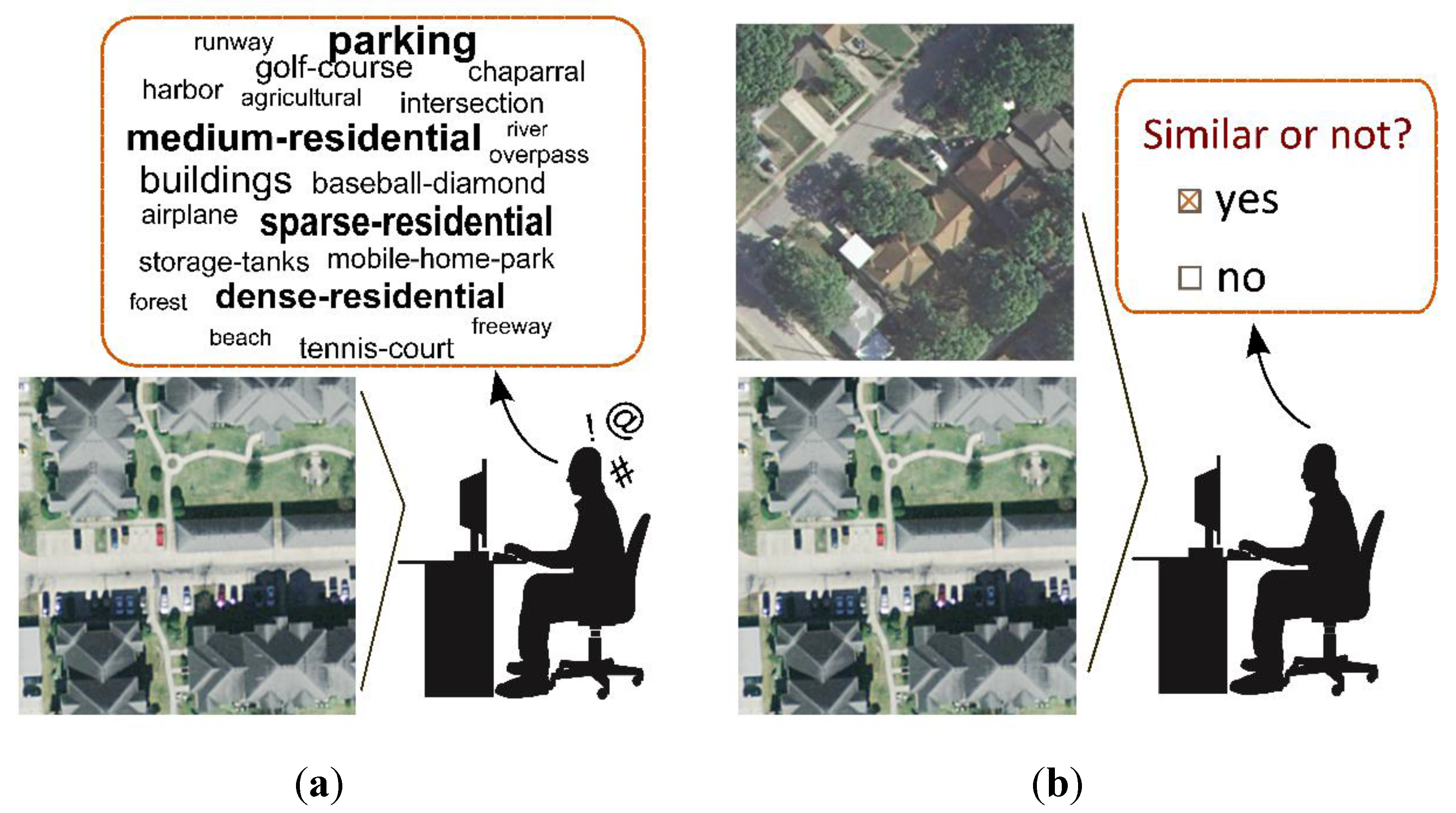
We develop an active clustering method for the annotation of HRRS images with little expert knowledge. When pairwise constraints are used as prior information, the human annotator is required only to compare pairs of remote sensing images and determine whether they are similar. This approach can alleviate the human workload requirements in terms of both quality and quantity as well as the requirement for human expert knowledge.
We define a novel weighted node uncertainty measure for selecting the informative nodes from a graph, which offers stable performance and sufficiently low algorithm complexity for the implementation of real-time human–computer interactions.
We propose an adaptive strategy that can automatically update the number of clusters in the active spectral clustering algorithm. This makes it possible to annotate remote sensing images when the number of categories, or their specific labels, is still unknown.
The remainder of this paper is organized as follows: Section 2 briefly describes several previously proposed approaches. Section 3 recalls some theoretical background. Section 4 introduces the proposed active spectral clustering framework for remote sensing images. Section 5 presents the experimental results. Section 6 and Section 7 offer some discussion and concluding remarks, respectively.

2. Related Work

The annotation of a remote sensing image refers to the process of assigning a certain semantic label to each element of the image. In accordance with the different types of image elements, there are two types of annotation: (1) Pixel-level annotation is the labeling of each pixel in the image, which is the classical approach for remote sensing images [12,13]. In fact, this approach is best suited for low- to mid-resolution remote sensing images, in which each pixel often corresponds to a large surface area; (2) Tile-level annotation is the assignment of a class label to each tiled image region, which is a more reasonable approach for HRRS images [17,18,19] because each semantic class label typically contains several sets of pixels, i.e., tiled image regions or super-pixels. In this paper, we are interested in the annotation of HRRS images and therefore focus on the tile-level annotation of images.
Traditional intelligent solutions to the annotation task for remote sensing images can be classified into two types depending on whether labeled data are provided: unsupervised methods [20,21] and supervised methods [7,9,22]. Methods of the former type attempt to discover the relationships among the original unlabeled data, and those of the latter type use the presented labeled data to learn a classifier to infer the labels of the unlabeled data. The two types of methods suffer from different problems, such as low accuracy and a high dependence on high-quality labeled data. This is because they use only part of the information available in the data (either the unlabeled data or the labeled data). In particular, although supervised classification methods perform well and are commonly used, they ignore the contributions from the unlabeled data, which typically constitute the majority of the available data.
In the case of remote sensing “big data”, labeled data are usually available; however, in contrast to the large volumes of unlabeled remote sensing images, the amount of available labeled data is still very limited, and their annotation demands considerable expert knowledge. Thus, the information of both the labeled and unlabeled data should be considered simultaneously. Furthermore, the quality of the supervised information provided by the labeled data is crucial. Highly redundant information and noise in labeled training data may lead to poor performance [23]. In other words, the appropriate selection of the labeled data is also necessary. To address these issues, semi-supervised learning and active learning algorithms have recently drawn considerable attention for remote sensing processing, not only in the annotation task [12,24,25,26,27] but also for change detection [28], image segmentation [29] and image retrieval [30,31].
Among these approaches, most of the methods that are focused on the annotation task use the framework of semi-supervised classification. These methods attempt to build an efficient training set, which contains as few labeled data as possible, to learn a reliable classifier. To achieve this purpose, there are three common types of strategies for intelligent sampling to select new labeled samples from a candidate pool of unlabeled samples [24]: (1) large-margin-based methods [32], which select candidates lying within the margin of the current support vector machine (SVM); (2) posterior-probability-based methods [33], which are based on the estimation of the posterior probability distribution function of the classes; and (3) committee-based methods [34], which train a set of classifiers using different hypotheses to label the candidates and select the most uncertain one. However, two difficulties are encountered with these algorithms when performing remote sensing image annotation: (1) These strategies rely on supervised models and require an initial training set, the construction of which is still based on negative selection (i.e., random sampling), and (2) the prior knowledge is typically provided in the form of class labels, for which the list of categories needs to be pre-defined.
Considering these two problems, active clustering [35,36,37,38,39], which melds active learning with semi-supervised clustering, is a better choice. In this approach, the clustering process can be initiated without any labeled data, and the method also offers high flexibility, with various species and means of using supervised information. For instance, using either class labels [27] (indicating exact categories) or pairwise constraints (indicating whether two samples belong to the same class) [40] as prior information is acceptable. In this sense, semi-supervised clustering is highly suitable for the analysis of remote sensing images, which is a task in which abundant unlabeled data and scant labeled data are typically available. Although various cluster-based active learning heuristics have recently been proposed [27] that rely on unsupervised models and can run without an initial training set, these methods still can only operate using class labels.
Most studies on active clustering have built upon traditional clustering methods, such as k-means [36,41,42] and hierarchical clustering [27,37,43]. A few active clustering algorithms based on spectral clustering, which can converge to global optimums [35,38,39], have also been developed. Different active selection strategies have also been adopted for these techniques. In one simple class of such strategies, active samples are directly selected according to their similarity values, as in the case of the farthest-first strategy [42] and the min-max criterion [36].
Moreover, several active strategies focus on deeper relationships between data, for instance, the boundary points and sparse points identified by examining the eigenvectors [38]. The authors of several studies have proposed pairwise active selection measures, such as the entropy of an example pair, to identify informative pairs [39]. Recently, Biswas et al. [37] chose the sample pair that maximized the change in the current clustering result to guide the clustering process to converge to a more suitable state. This pairwise criterion is reasonable, but it requires the evaluation of n2 pairs in each iteration and is therefore slow. Xiong et al. [35] proposed to gradually purify a k-NN graph of data during spectral clustering using a cutting process, in which an entropy-based node uncertainty measure is applied to select the most informative samples. This algorithm is fast and performs well, but when the neighborhood size (i.e., the k of the k-NN graph) is small, one can observe that (1) the node uncertainty measure may lose efficiency and (2) the algorithm may not converge to a robust state with only a single cutting process. It is also worth noting that none of these algorithms can handle the case in which the number of clusters is unknown, which is very common in real applications.
This paper proposes an active spectral clustering (ASC) method with pairwise constraints for the annotation of remote sensing images. With a weighted sample-based active selection criterion and a two-step graph purification process, ASC exhibits improved robustness to k-NN graphs with different structures. Moreover, an adaptive version (AASC) is also proposed, which can adaptively determine the number of clusters during iteration and performs equally as well as ASC.

3. Background on the Annotation of Remote Sensing Images

This section provides some theoretical support for our work. We first briefly recall the basis of spectral clustering and then introduce how to compute the similarity matrix in the clustering procedure for HRRS images.
Given a set of HRRS image data = { I i } i = 1 N , the annotation of Ii is the assignment of a semantic label l m = { l 1 , , l M } to it in accordance with its content (land use or land cover). This paper concentrates on the tile-level annotation of remote sensing images. However, note that our method takes a general setting and can also be used for the pixel-level annotation of remote sensing images if one defines each pixel as a tile.

3.1. Spectral Clustering

Spectral clustering [44] is based on spectral graph theory. It uses a graph structure to exploit the intrinsic characteristics of a set of data and transforms a clustering problem into a graph partitioning problem. In contrast to many traditional clustering algorithms (e.g., k-means or single linkage), spectral clustering demonstrates great superiority because of its efficiency and its simplicity of implementation [45].
Constructing a k-NN graph: Given a set of image data (pixels or regions) = { I i } i = 1 N , the similarity matrix W = { w i j } i , j = 1 N of is calculated as follows: wij = sim (Ii,Ij),
where each element wij indicates the similarity between Ii and Ij. The similarity function sim (,) will be described later in this section.
The similarity graph of the dataset is thus defined as G = (V, E), where the vertex v i V represents a data point Ii and where any two vertices Ii and Ij are linked by an edge eij with a weight of wij. As we know, a fully connected n-vertex graph contains n (n − 1)/2 edges, most of which are not actually necessary for later work but merely degrade the efficiency. One effective method of constructing such a graph G is to use a k-NN graph, which retains, for each vertex, only the edge linked to the k most similar other vertices in the fully connected similarity graph.
Spectral clustering algorithm: Different spectral clustering algorithms can be distinguished by their use of the graph cut strategy and the objective function [44], such as
min N C u t ( G 1 , G 2 ) = c u t ( G 1 , G 2 ) v o l ( G 1 ) + c u t ( G 1 , G 2 ) v o l ( G 2 ) ,
where G1 = {V1, E1} and G2 = {V2, E2} are two disjoint subgraphs of G that satisfy V 1 V 2 = V and V 1 V 2 = and where
c u t ( G 1 , G 2 ) = i V 1 , j V 2 w i j
v o l ( G 1 ) = i V 1 , j V w i j ,        v o l ( G 2 ) = i V 2 , j V w i j
This minimization problem is NP-hard, whereas its relaxation is tractable. In [45], a normalized Laplacian matrix Lsym of the undirected graph G is constructed as follows:
L s y m = I D 1 / 2 W D 1 / 2
where I is the identity matrix and D is the diagonal matrix defined by D i i = j = 1 N w i j . Spectral clustering is then applied to the first several (e.g., a number of classes m) eigenvectors of the normalized Laplacian matrix Lsym, relying on the k-means algorithm.
To address large-scale remote sensing image data, certain large-scale spectral clustering algorithms will take less time to perform the clustering. The underlying spectral clustering forms the basic structure of our method. Here, we use the Ng-Jordan-Weiss (NJW) algorithm [45].

3.2. Characterization and Similarity of Remote Sensing Images

A key step in the implementation of spectral image clustering is to construct the graph G. Let = { I i } i = 1 N be a set of remote sensing image data, each of which is described by a visual feature vector fi, e.g., spatial location, intensity, color, texture or other more comprehensive features. In our case, to characterize a remote sensing image Ii, we concatenate the bag-of-dense-SIFT descriptors [46] and bag-of-color descriptors [47] to form the feature vector, following the scheme of the bag-of-words model [48]. Note that the representative power of our scheme can be further improved by employing other comprehensive features, e.g., mid-level structures [49,50] and structural texture descriptors [51,52].
Because the vector fi is a histogram-like feature, we use the histogram intersection kernel (HIK) [53] as the similarity function,
s i m ( I i , I j ) = z min ( f i [ z ] , f j [ z ] )
where fi [z] indicates the z-th bin of the histogram vector fi. The similarity measure defined in Equation (5) takes values between 0 and 1. The k-NN graph is then constructed based on this similarity matrix W.

4. Methodology

4.1. Active Spectral Clustering of Remote Sensing Images

Spectral clustering is performed based on the graph constructed from the data of interest. It has been reported, based on a theoretical convergence analysis of spectral clustering, that the structure of the graph may have a considerable impact on the clustering result [45]. In [54], the authors introduced a general framework to analyze graph constructions by shrinking the neighborhoods of a k-NN graph. In short, a k-NN graph whose neighbors are more certain could generate a better clustering result.
Definition 1. (Perfect k-NN graph): A k-NN graph G = (V, E) is said to be perfect if e i j , if eij = 1, then li = lj, i.e., the connected nodes vi and vj have the same label.
It is worth noting that for a perfect k-NN graph, each vertex and all of its k neighbors belong to the same class. Obviously, a typical graph of data is far from perfect, and there are many “abnormal neighbors” and “abnormal edges”, which are defined as follows.
Definition 2. (Abnormal neighbor): For a node v i V vi in the graph G = (V, E), an “abnormal neighbor” of the node vi is a node vj that does not have the same label as vi but for which the similarity wij between them is sufficiently abnormally large for vj to be included in the neighborhood of vi.
Definition 3. (Abnormal edge): An “abnormal edge” is an edge linking to an abnormal neighbor vj.
Note that the purpose of graph-based spectral clustering is to pursue such a perfect or near-perfect k-NN graph from a given set of data. In what follows, we introduce an online algorithm that iteratively revises a k-NN graph by removing “abnormal edges”, i.e., edges that link two vertices of different classes that would not appear in a perfect k-NN graph. To achieve this goal, we iteratively obtain new constraints by actively selecting the most informative image pair and querying an oracle (such as a human annotator).
The flowchart of the algorithm is depicted in Figure 2. Given a set of images (or image regions) as inputs, we first construct the k-NN graph and then apply a spectral clustering algorithm, as described in Section 3. Active learning helps us to identify the most informative image, which is also the most uncertain one, based on the current clustering result and the k-NN graph. Using the new constraints, the k-NN graph is purified, and spectral clustering is then performed again on the new k-NN graph. The algorithm iterates this process until the oracle is satisfied or until the k-NN graph is fully purified. We will describe each part of our algorithm in detail below.
Figure 2. Flowchart for the active spectral clustering of remote sensing images. Given a set of images (or image regions) as inputs, we first construct the k-nearest neighbor (k-NN) graph and then apply a spectral clustering algorithm, as described in Section 3. Active learning helps us to identify the most informative image, which is also the most uncertain one, based on the current clustering result and the k-NN graph. Using the new constraints, the k-NN graph is purified, and spectral clustering is then performed again on the new k-NN graph. The algorithm iterates this process until the oracle is satisfied or until the k-NN graph is fully purified. Refer to the text for more details.
Remotesensing 07 15014 g002

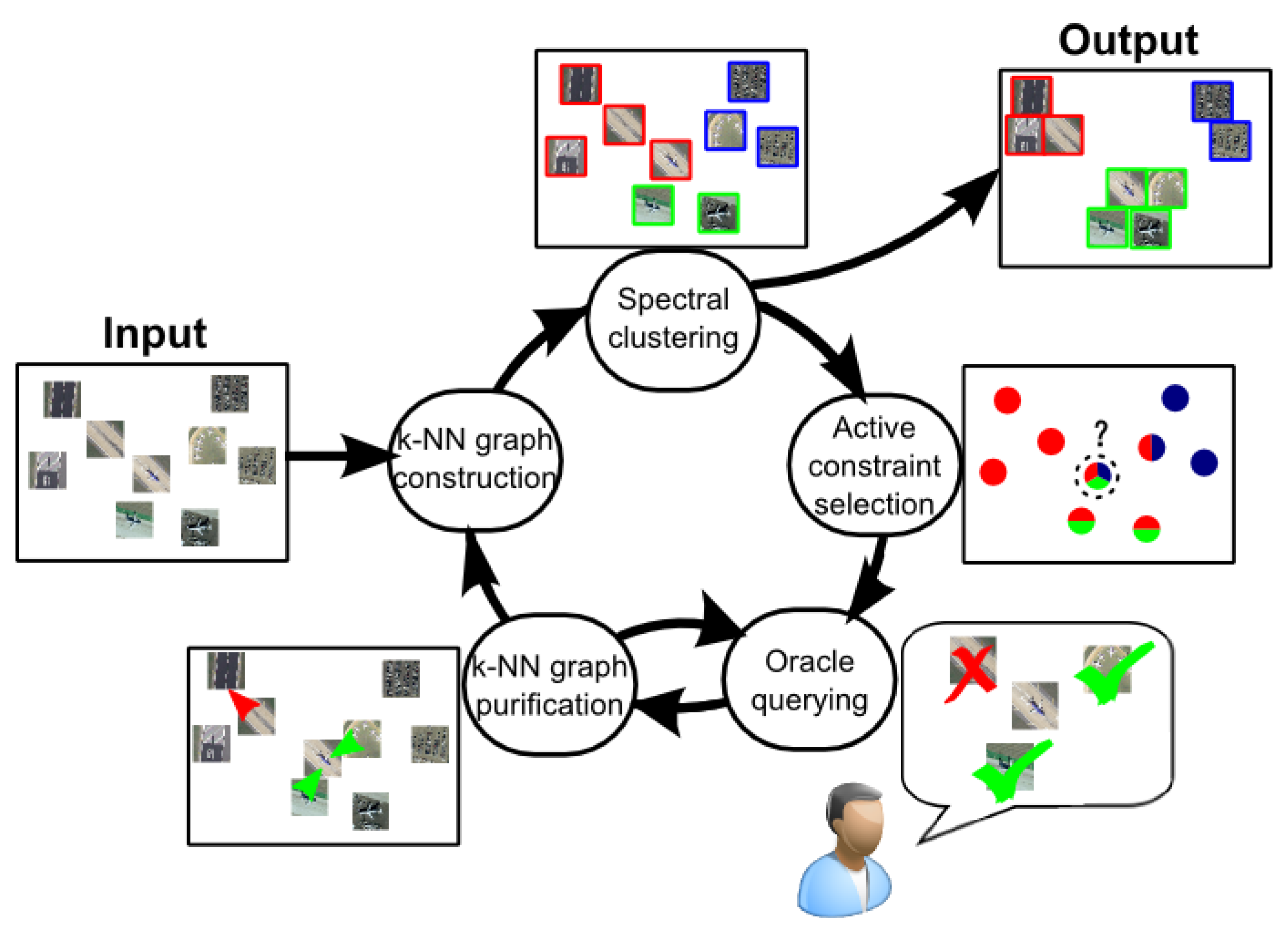
4.1.1. k-NN Graph Construction and Basic Spectral Clustering

The first step is to construct a k-NN graph from the data as described in Section 3. Again, we choose the NJW algorithm [45] as our basic spectral clustering algorithm.

4.1.2. Active Constraint Selection

In this step, we use active learning to select useful constraints. Recalling the construction of the k-NN graph, for each node, only the edges linked to its k nearest neighbors are retained, meaning that the relationships of the remote sensing image samples are actually approximately represented by each sample and its k nearest samples. In the ideal case, each image sample should have a high similarity with and the same class label as its neighbors. Consequently, nodes that are connected in the k-NN graph will be assigned to the same cluster. Based on this analysis, the proposed active selection strategy is to identify the abnormal neighbors and eliminate them from the neighborhoods, implying the removal of “abnormal edges” from the k-NN graph.
However, because the real class labels of the nodes are still unavailable, we cannot directly search for these abnormal neighbors. Therefore, instead of using the real class labels, we use the current cluster labels and perform active learning using the current k-NN graph.
Figure 3. Active constraint selection process: selection of the most uncertain node based on the current k-NN graph and the clustering result. (a) The current k-NN graph, in which different clustering labels are represented by differently colored frames. (b) The selection of the most uncertain node.
Remotesensing 07 15014 g003
In the spectral clustering scheme, the label of a given node depends on the labels of its k neighbors. When the neighbors of Ii have many different labels and are disordered, it is difficult to assign Ii a particular label. For example, consider the center node in Figure 3a, where the neighbors of the node are assigned to three different clusters. Its label is quite uncertain, although it is assigned to the red cluster. The neighborhood of this node is more likely to contain abnormal neighbors and abnormal edges.
According to the analysis above, it is important to actively identify the most uncertain node in the k-NN graph. First, we compute the probability of Ii being assigned to cluster as follows:
P ( I i | ) = I j N i w i j δ ( l j , ) I j N i w i j
where N i is the neighborhood (neighbor set) of Ii, lj is the cluster label of Ii, wij is the edge weight (similarity) between Ii and Ij, and δ ( l j , ) is a binary function that takes a value of 1 when l j = and is equal to 0 otherwise. Here, the probability P ( I i | ) is computed as the ratio of the edge weights that are assigned to the cluster . Note that this definition is different from that given in [35], where equal weights were used to compute the probability. As we shall see in our experiments, our definition is more robust with respect to the neighborhood size.
Similar to [35], we use an entropy criterion to measure the level of uncertainty of node Ii:
H ( I i ) = P ( I i | ) log P ( I i | )
where P (Ii/ ) is the probability computed above. The image I i * with the highest entropy is chosen, indicating that the cluster labels inside its neighborhood are the most disordered:
I i * = arg max H ( I i ) .
Note that our algorithm is performed online. To avoid selecting nodes that have been used in previous iterations, Equation (8) is modified as follows:
I i * = arg max I i I h H ( I i ) ,
where Ih is the set of nodes that have already been selected.

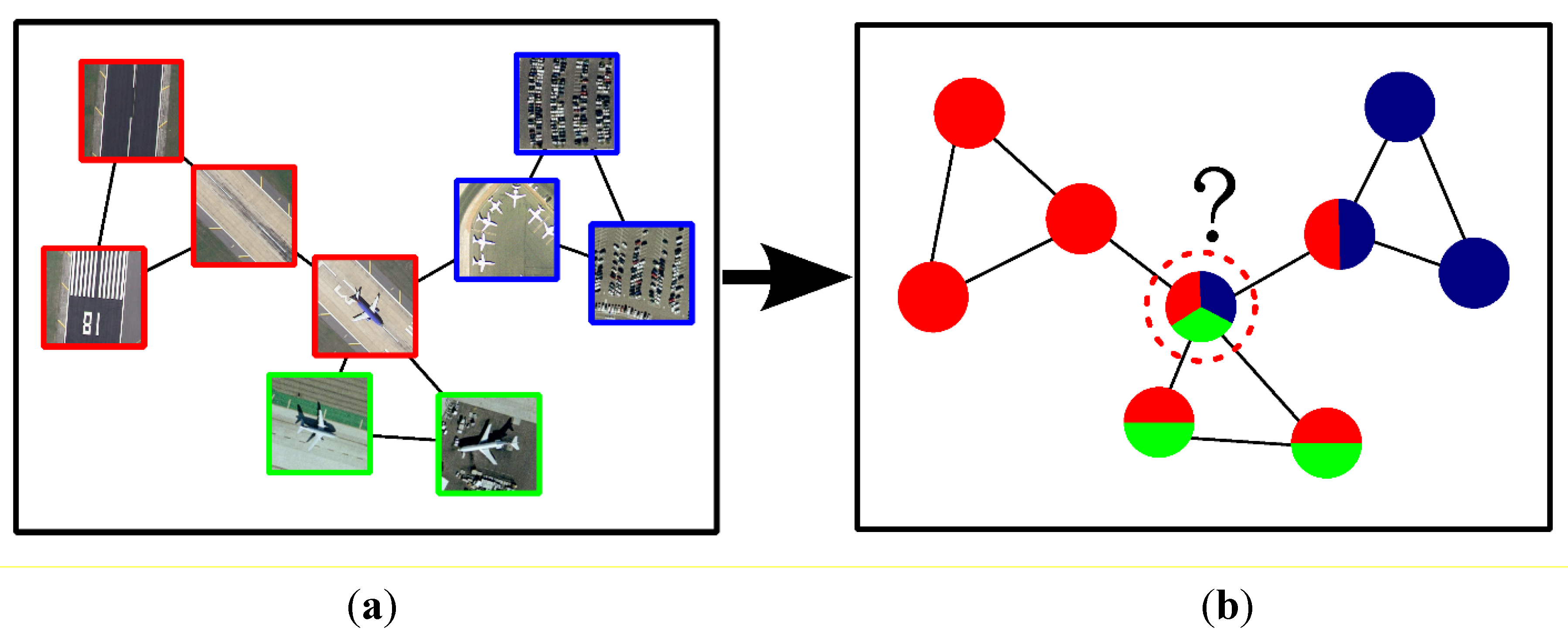
4.1.3. Oracle Querying
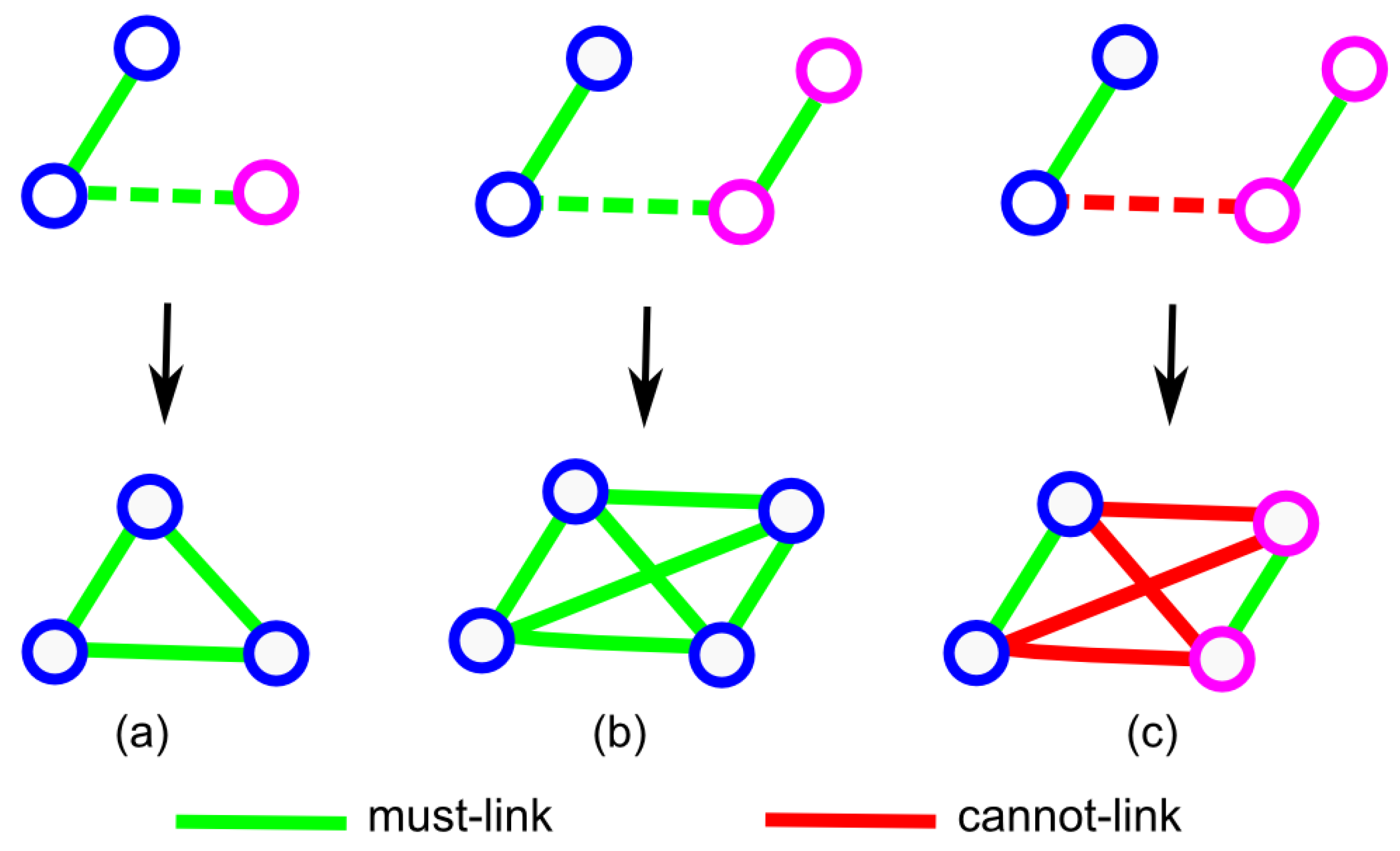
Based on the identification of the most uncertain node Ii, several candidate edges are selected (as described in the k-NN graph purification step) to query an oracle. The algorithm presents the images that are linked by these candidate edges and queries the oracle (such as a human annotator) regarding whether they are similar. The oracle can compare the two images and easily provide the answer. Based on the simple feedback of “yes” or “no”, the algorithm can obtain a set of pairwise constraints: must-links (the linked images must belong to same class) and cannot-links (the linked images must belong to different classes).
Note that pairwise constraints are transitive. A simple constraint augmentation process is described in Figure 4 to obtain additional constraints from the known constraints:
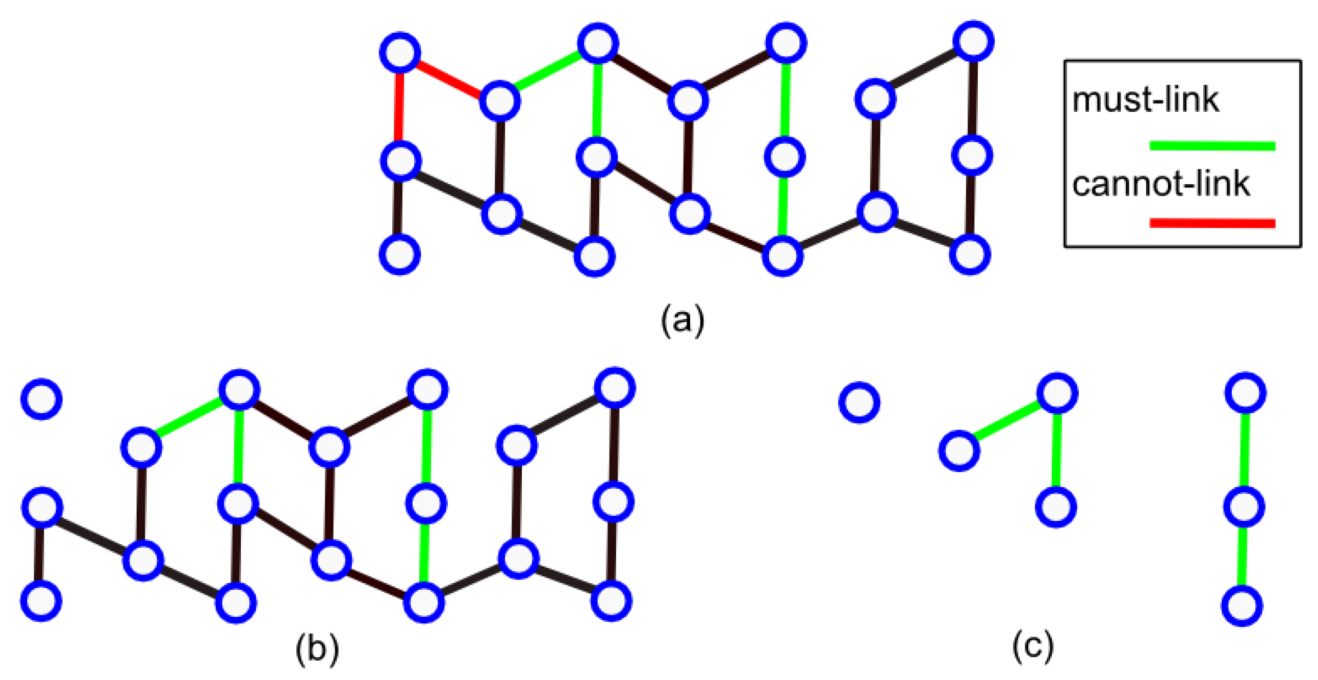
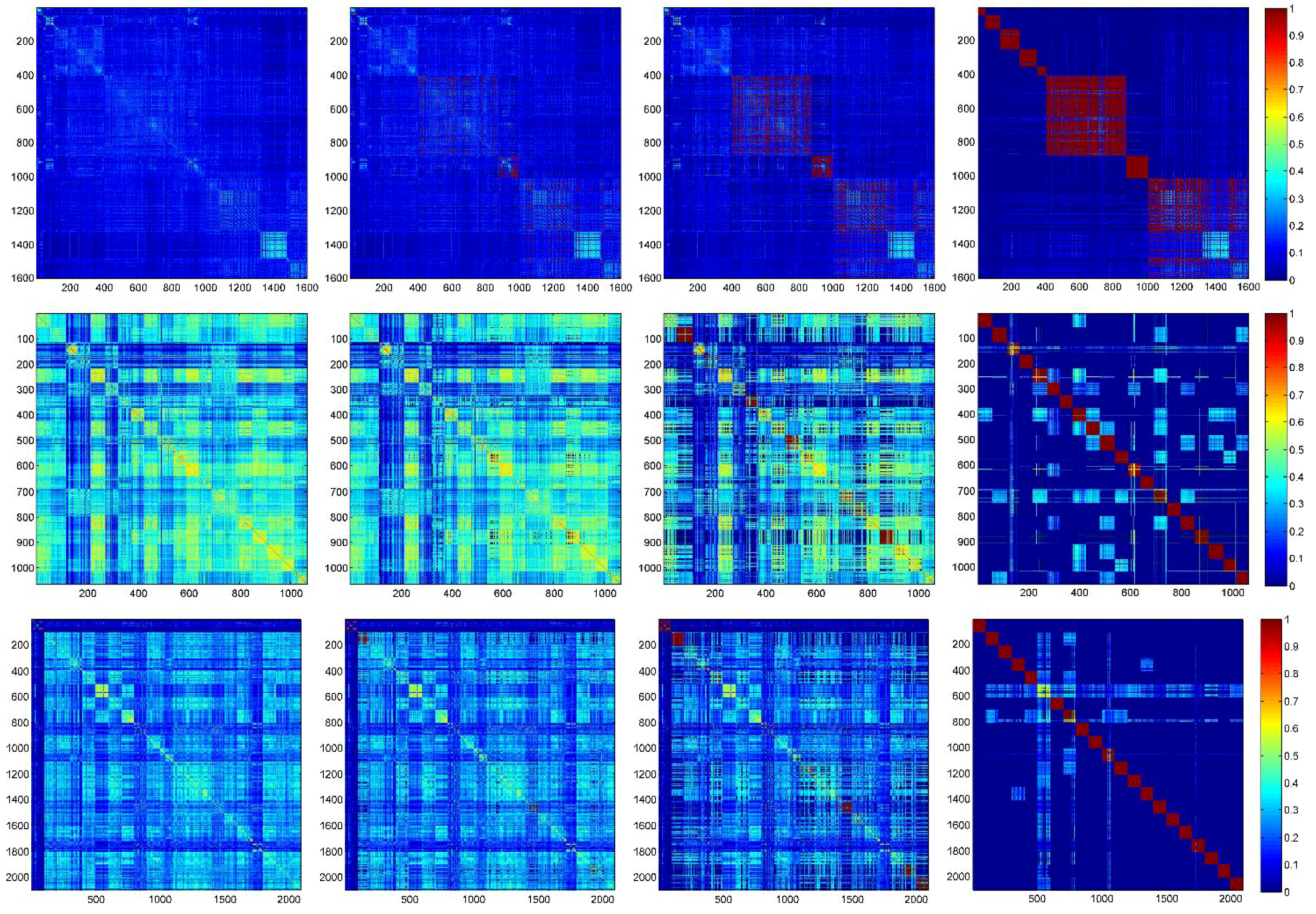
All nodes in a single connected component formed by must-links should belong to the same class and be linked to each other by must-links. These fully connected components are called cliques in graph theory (see Figure 4a).
If a must-link exists between two cliques, then they should be merged and must-links should be added between their component nodes (see Figure 4b).
If a cannot-link exists between two cliques, then they should belong to different classes and cannot-links should be added between their component nodes (see Figure 4c).
Figure 4. Constraint augmentation process. A solid line represents a previously known constraint, and a dotted line represents a newly added constraint.
Remotesensing 07 15014 g004

4.1.4. Two-Step k-NN Graph Purification Process

In fact, the steps of k-NN graph purification and oracle querying proceed concurrently. Based on the most uncertain node Ii, several candidate edges are selected to query the oracle. Using the oracle’s feedback, the candidate edges can be transformed into pairwise constraints and used to purify the current k-NN graph.
The k-NN graph purification procedure consists of two steps: Cut and Collect.
The purpose of the Cut process, as shown in Figure 5, is to remove abnormal edges from a k-NN graph. The edges in the neighborhood N I * of I i * are chosen as candidate edges that are likely to be abnormal ones, denoted by
E ( I i * ) = { ( I i * , I j ) | I j N i }
Using the oracle’s feedback, these candidate edges may be transformed into either must-links or cannot-links. In our case, we directly purify the k-NN graph: all cannot-link edges in the graph will be removed, whereas the must-links will be strengthened (the similarity value of each associated edge will be re-weighted to 1).
However, as seen from Figure 5b, in this process, certain nodes or cliques may become disjointed from the graph. Because spectral clustering considers only the graph cut problem, the relationships between these discrete components and the remainder of the graph are lost, and they may be regarded as clusters themselves. To overcome this problem, another process, termed the Collect process, is needed.
Figure 5. Cut process: (a) k-NN graph before Cut; (b) k-NN graph after Cut; and (c) discrete components.
Remotesensing 07 15014 g005
The purpose of the Collect process, as shown in Figure 6, is to identify the discrete components created in the Cut process and relink them to the k-NN graph. In addition to these discrete nodes and cliques, we construct a set S = {S1,S2,…,Sr}to collect all cliques obtained from must-links. Here, r is the number of subsets, and each subset Sl of S corresponds to a certain set of nodes belonging to the same cluster. This set is initialized with r = 0 and S = Ø.
After each Cut process, several discrete components may be produced. We wish to incorporate these discrete components into S one by one. More precisely, the first discrete component set Dc1 is simply added as S1, and r is updated to r = 1. Subsequently, when a new discrete component Dc is generated, it is successively compared to the subsets that are most similar to it. The similarity of v and Sp is described in terms of the mean weight of the edges between them, as follows:
s i m ( D c , S p ) = I i D c , I j S p w i j I i D c , I j S p 1
The sample pair ( I i , I j ) | I i D c , I j S i with the largest wij is then selected as the candidate pair. Through oracle querying, the relationship between Dc and Sp is determined. If they belong to the same class, then Dc is added into Sp; otherwise, Dc is compared to another subset. If Dc cannot be incorporated into any existing subset, then we construct a new subset Sr+1 and update r as r r + 1 .
In more evocative terms, we collect and package discrete components into bags of certain categories. When a new type of discrete component is encountered, we pack it into a new bag. Through the Collect process, each discrete component will find a subset to which it belongs. Because different subsets Sp correspond to different classes, must-links will be added between vertices of the same subset, whereas cannot-links will be added between different subsets. Through this process, discrete components will ultimately become linked to the graph once again.
Figure 6. Collect process: Add a new discrete component to a subset of S or construct a new subset if necessary.
Remotesensing 07 15014 g006

4.1.5. Stopping Criterion

The question of when to terminate the active learning algorithm is actually quite a practical problem. One purpose of active learning is to reduce the cost of labeling. Thus, it is not necessary to continue once the result has converged or has achieved a sufficient quality that the attempt to obtain a better result is no longer worth the cost. In practical applications, the stopping criterion is often related to economic or other factors, such as the maximum number of iterations tmax [15]. Because the quality of the result cannot be measured without a ground truth, here we define the steady iteration τ to describe the contributions of the current newly added constraints.
Definition 4. (Steady iteration τ): The number of subsequent iterations in which the cluster labels remain the same with no constraints being broken.
Obviously, a larger value of τ indicates less useful constraints. Thus, we can define a threshold ϵ and terminate the algorithm when τ > ϵ . We set ϵ = 10 in the experiments presented in Section 5.

4.1.6. Pseudocode

After the purification of G(t), a new k-NN graph G(t+1), is constructed and used to perform spectral clustering in the next iteration. The algorithm iterates this process until the result is satisfactory or τ > ϵ . The detailed algorithm is summarized in Algorithm 1.
Algorithm 1. ASC: 
Active Spectral Clustering of Remote Sensing Images
Input: 
Image dataset = { I 1 , I 2 , , I n } ; Number of clusters m; Maximum number of iterations tmax; Threshold of steady iteration ϵ
Output: 
Labels Y = { l 1 , l 2 , , l n }
  • Initialization: extract features from images , measure the similarities between images, and construct the k-NN graph G(0); set t = 0;
  • repeat 
  • perform spectral clustering on the current graph G(t) to obtain the set of clustering labels Y ( t ) = { l 1 ( t ) , l 2 ( t ) , , l n ( t ) } ;
  • Active selection: compute I i * = arg max I i I h H ( I i ) and incorporate Ii into Ih;
  • Querying and construction of G(t+1):
    Cut process: remove the cannot-links from G(t) and set the weights of the must-links to 1;
    Collect process: collect the newly disconnected graph components into the set S = {S1,S2,…,Sr} and construct G(t+1).
  • update t t + 1
  • update τ
  • until τ > ϵ or t t m a x
  • Y = Y ( t )

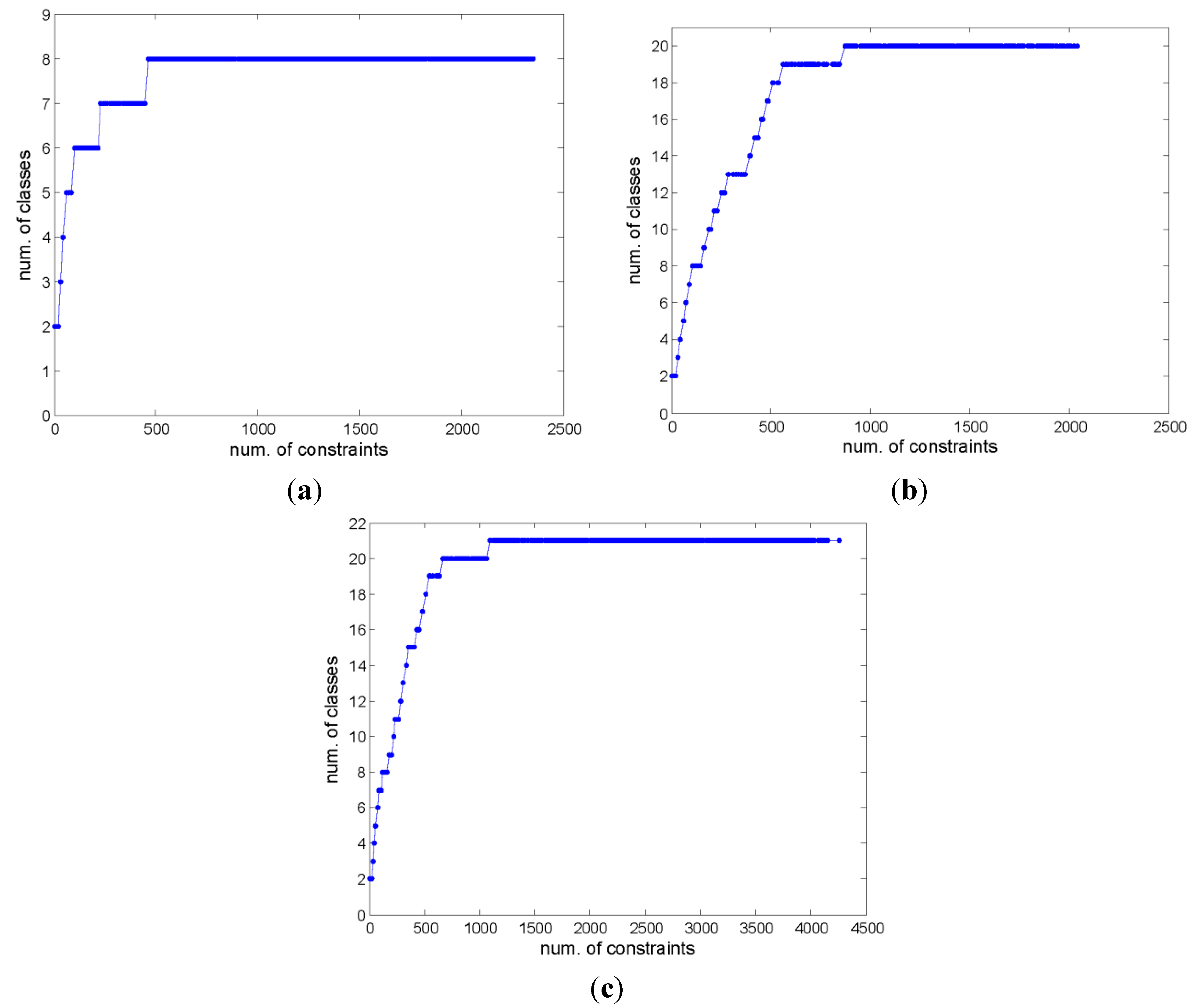
4.2. Adaptive Active Spectral Clustering of Remote Sensing Images

In our ASC algorithm proposed above, the number of clusters m is required as an input parameter. This scenario is common for the annotation of remote sensing images when all categories are predefined. However, realistically, it is often difficult to determine the number of scene classes contained in remote sensing images when there is no prior information. For example, in the annotation of large-volume remote sensing images, it is generally difficult to obtain an overview of the entire dataset that is sufficient to pre-define all categories. To address this scenario, this section presents an improved algorithm called adaptive active spectral clustering (AASC), in which the number of clusters can be adaptively determined.
Note that in the “Collect” step of ASC, we construct S as a number of bags in which to aggregate discrete components. In the AASC algorithm, to adaptively set the number of clusters m, we use the number of subsets r to update m. More precisely, we initialize r = 2 and set m= max (r, 2). The remainder of AASC is identical to ASC. During the operation of the AASC algorithm, m will be updated when additional mutually exclusive clusters are found. The experiments presented in Section 5 demonstrate that the AASC algorithm can adaptively determine the real number of clusters. The improved algorithm is summarized in Algorithm 2.
Algorithm 2. AASC: 
Adaptive Active Spectral Clustering of Remote Sensing Images. 
Input: 
Image dataset = { I 1 , I 2 , , I n } ; Maximum number of iterations tmax; Threshold of steady iteration ϵ
Output: 
Labels Y = { l 1 , l 2 , , l n }
  • Initialization: extract features from images , measure the similarities between images, and construct the K-NN graph G(0); set t = 0 and set the number of clusters m = 2;
  • repeat 
    perform spectral clustering on the current graph G(t) to obtain the set of clustering labels Y ( t ) = { l 1 ( t ) , l 2 ( t ) , , l n ( t ) } ;
  • Active selection: compute I i * = arg max I i I h H ( I i ) and incorporate I i * into I h ;
  • Querying and construction of G(t+1):
    Cut process: remove the cannot-links from G(t) and set the weights of the must-links to 1; 
    Collect process: collect the newly disconnected graph components into the set S = {S1,S2,…,Sr} and construct G(t+1).
  • update m max ( r , 2 )
  • update t t + 1
  • update τ
  • until τ > ϵ or t t m a x
  • Y = Y ( t )

5. Experiments

5.1. Description of the Datasets

To evaluate the performance of the proposed algorithm introduced in Section 4.1 and Section 4.2, this section presents several experiments on three real HRRS datasets:
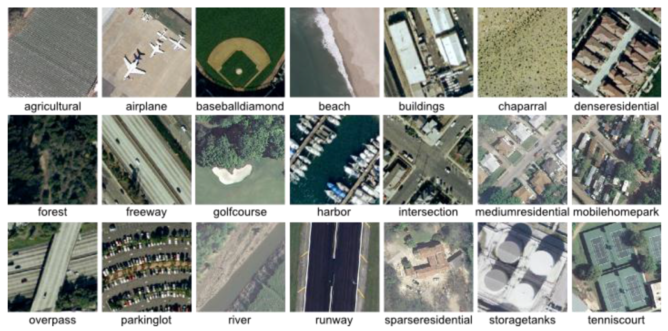
UC Merced (UCM) Dataset [47]: This dataset consists of 21 scene categories (including land-cover classes, e.g., forest and agricultural, and object classes, e.g., airplanes and tennis courts) with a pixel resolution of one foot. Each class contains 100 images with dimensions of 256 × 256 pixels. Examples from each class in the dataset are shown in Figure 7.
WHU-RS Dataset [55]: This dataset contains 1063 HRRS images in a total of 20 classes, e.g., airports, mountains, and residential areas; see Figure 8. The size of each sample is 600 × 600 pixels.
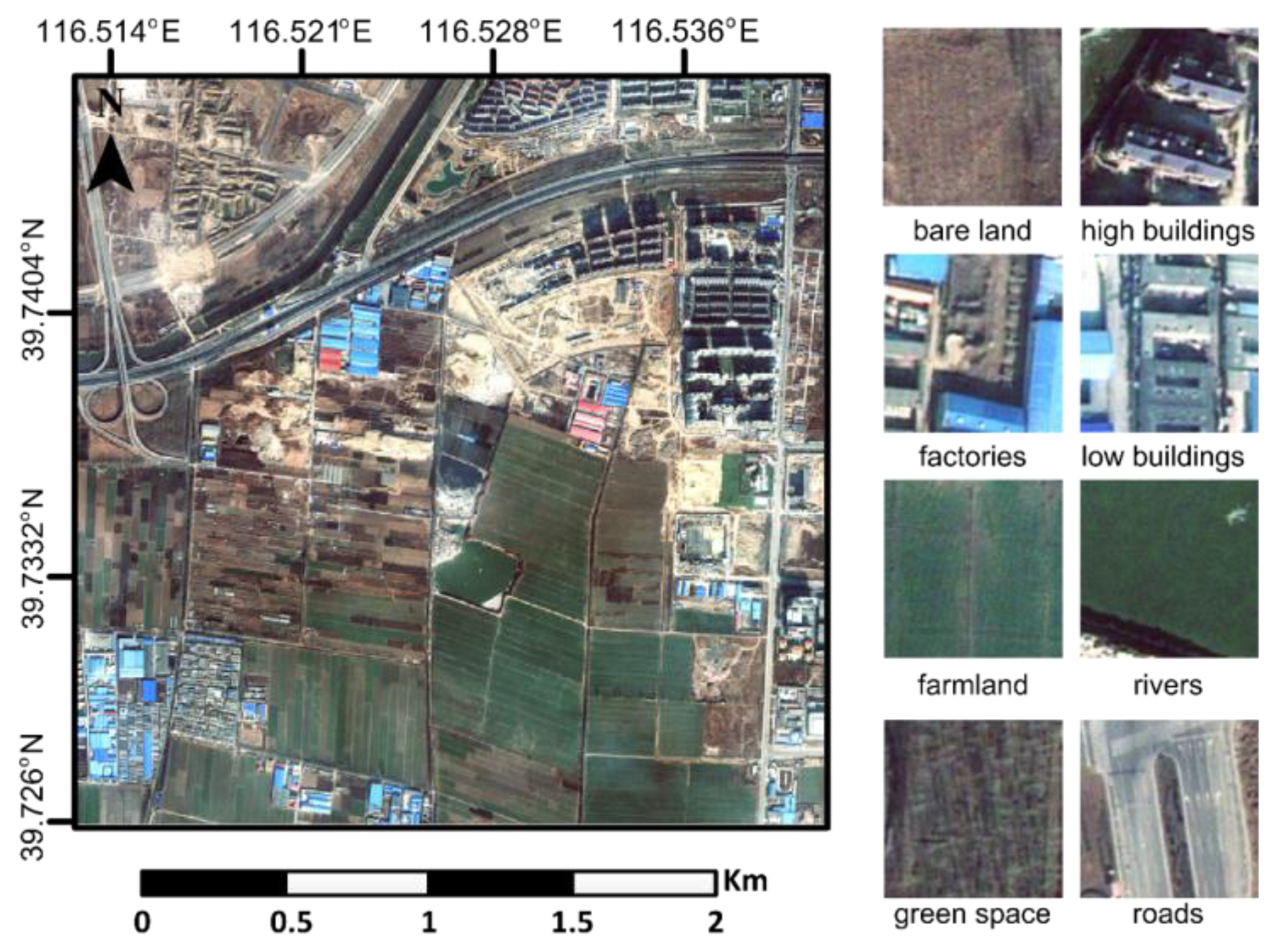
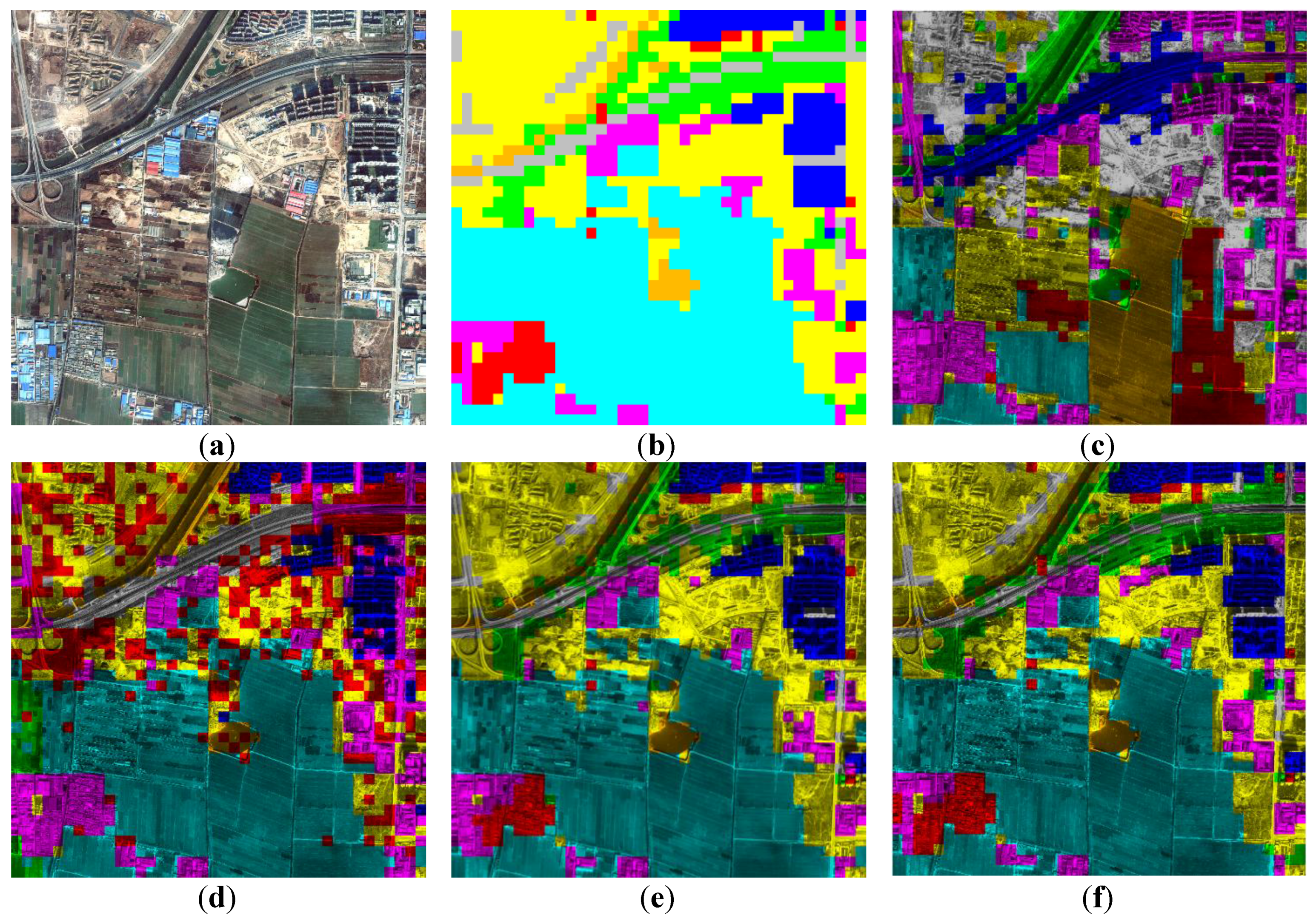
Beijing Dataset [17]: This dataset consists of a large high-resolution satellite image captured by GeoEye-1 of Majuqiao Town, located in the southwest Tongzhou District in Beijing. The original image, with dimensions of 4000 × 4000 pixels, is cut by a uniform grid into regions with dimensions of 100 × 100 pixels. These 1600 image regions are annotated with 8 classes (such as bare land, factories, and rivers). The original image and a sample from each class are shown in Figure 9.
Figure 7. Examples of each category from the UCM dataset.
Remotesensing 07 15014 g007
Figure 8. Examples of each category from the WHU-RS dataset [55].
Remotesensing 07 15014 g008
Figure 9. Original image of the Beijing dataset. The size of the raw GeoEye-1 image is 4000 × 4000 pixels. Examples from each category are shown on the right.
Remotesensing 07 15014 g009

5.2. Experimental Setting

Note that the proposed ASC and AASC algorithms rely on K-means and are stochastic. Thus, to verify the stability of our method, we report multiple experiments below (50 runs each) and report the mean accuracy and standard deviations achieved using the investigated algorithms.

5.2.1. Evaluation Measures

Clustering algorithms ultimately output a set of clustering labels, which often do not correspond to real semantic labels. Therefore, it is difficult to directly judge which result is superior. Many methods of evaluation have been proposed to measure the performance of such algorithms. Here, we adopt two well-known measures: the Jaccard coefficient [56] and the V-measure [57].
The Jaccard coefficient measures clustering performance by computing the ratio of correctly assigned sample pairs:
J C C = S S S S + S D + D S
where SS indicates the total number of same-class pairs that are assigned to the same cluster, DS indicates the total number of different-class pairs that are assigned to the same cluster, and SD is the total number of same-class pairs that are assigned to different clusters.
The V-measure is an entropy-based cluster evaluation measure. It calculates the harmonic mean of satisfaction of the homogeneity h and completeness c, which are two desirable aspects of correspondence between a set of classes C (ground truth) and a set of clusters K. Let apq be the number of data samples that are members of class q and assigned to cluster p. The homogeneity h is defined as
h = { 1 if  H ( C , K ) = 0 1 H ( C | K ) H ( C ) else
where H ( C | K ) = p = 1 | K | q = 1 | C | a q p N log a q p q = 1 | C | a q p , H ( C ) = q = 1 | C | p = 1 | K | a q p N log p = 1 | K | a q p N .
The completeness c is defined as
c = { 1 if  H ( K , C ) = 0 1 H ( K | C ) H ( K ) else
where H ( K | C ) = q = 1 | C | p = 1 | K | a q p N log a q p p = 1 | K | a q p , H ( K ) = k = 1 | K | q = 1 | C | a q p N log q = 1 | C | a q p N .
Finally, the V-measure computes the harmonic mean of h and c:
V β = 2 h c h + c
The values of both the Jaccard coefficient and the V-measure lie in the range (0,1). A larger value indicates a more accurate result. A perfect clustering result is achieved when the value is equal to 1. It is also worth noting that Jaccard coefficient is a pair-matching measure, which may suffer from distributional problems, and the V-measure has been reported to be more robust in this sense [51].

5.2.2. Comparison Baseline and State-of-the-Art Methods

To test our active spectral clustering algorithms for the annotation of remote sensing images, we will compare our methods with several related approaches, including a baseline and several state-of-the-art multi-class active clustering algorithms:
Random: A baseline algorithm that is similar to the proposed ASC algorithm but randomly samples pairwise constraints rather than using active learning.
RandomA: A baseline algorithm that is similar to the proposed AASC algorithm but randomly samples pairwise constraints rather than using active learning.
CCSKL [58]: A constrained spectral clustering algorithm that uses spectral learning and randomly sampled pairwise constraints.
PKNN [35]: An active spectral clustering algorithm that also iteratively refines a k-NN graph.
HACC [37]: An active and hierarchical clustering method that selects the pairwise constraints that lead to the maximal expected change in the clustering results.
ASC: Our proposed active spectral clustering algorithm for remote sensing images, described in Section 4.1.
AASC: Our proposed adaptive active spectral clustering algorithm for remote sensing images, described in Section 4.2.

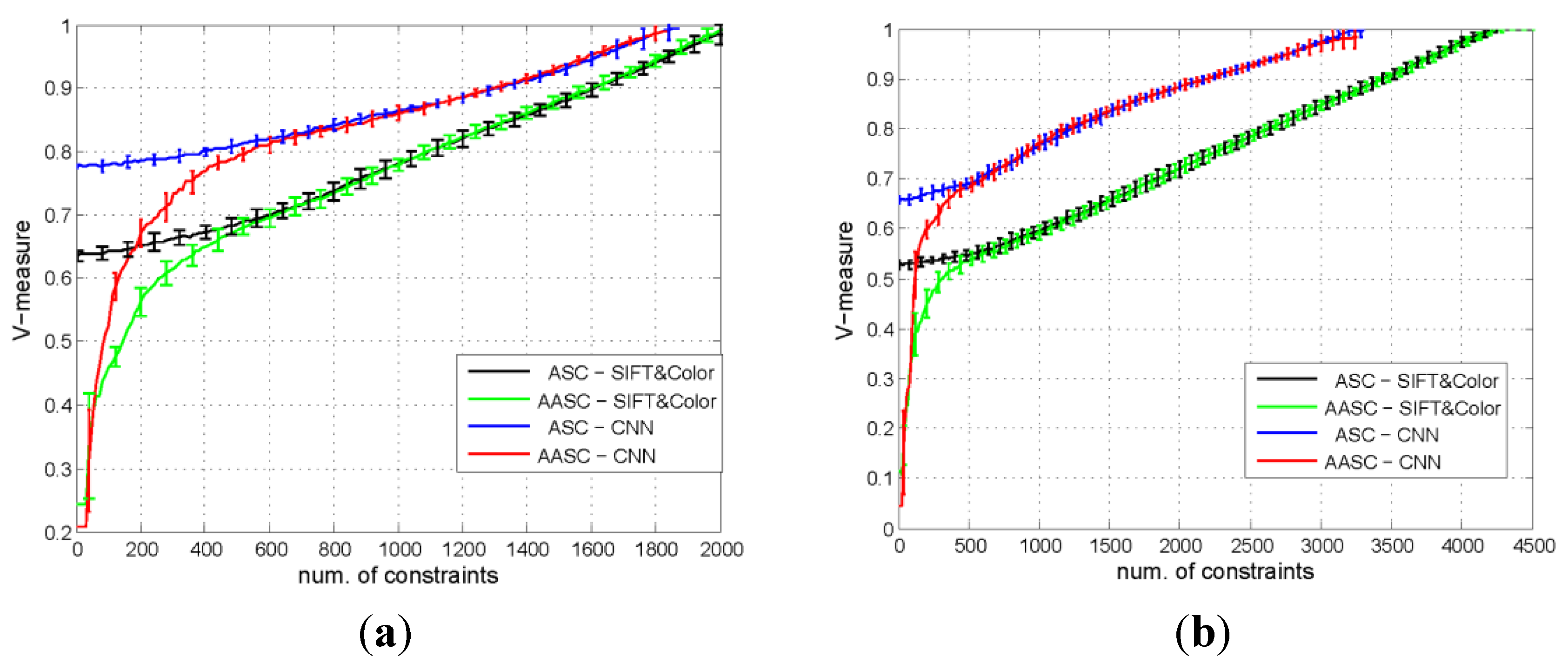
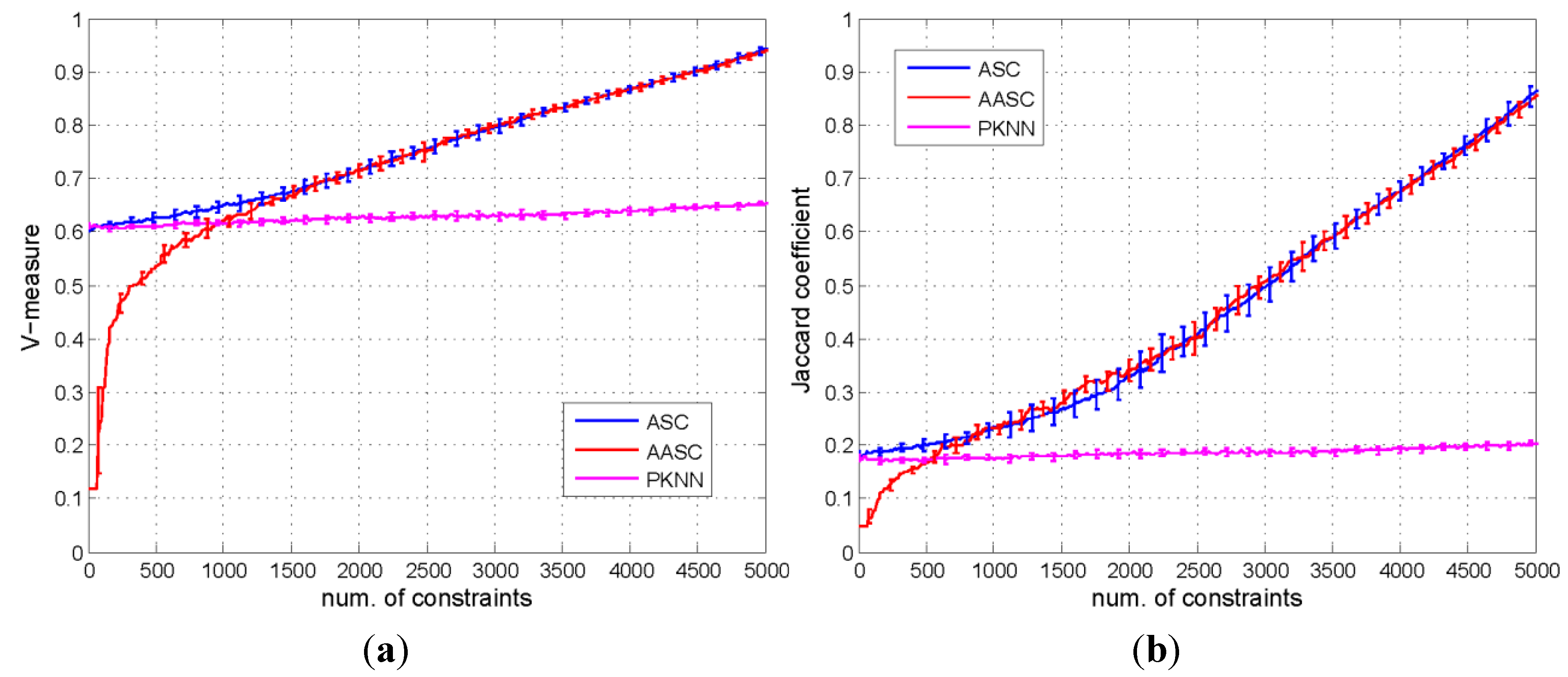
5.3. Experimental Results and Analysis

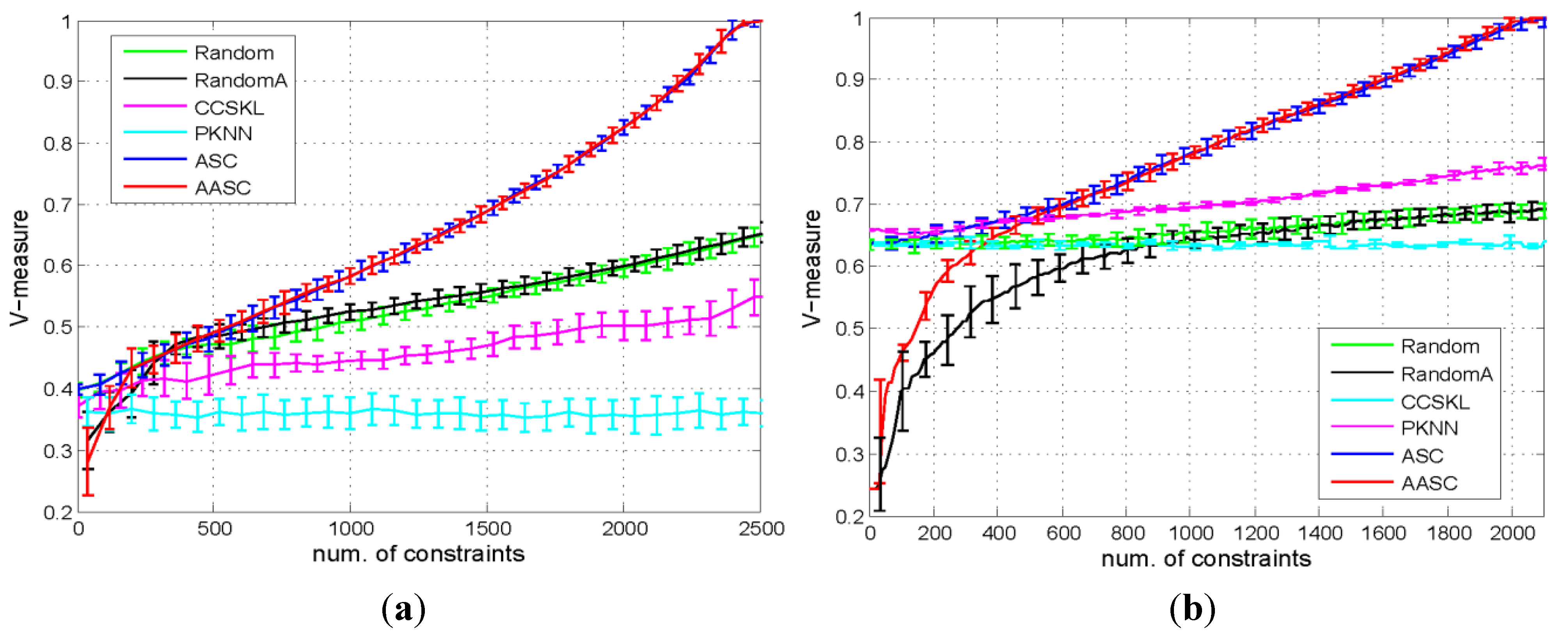
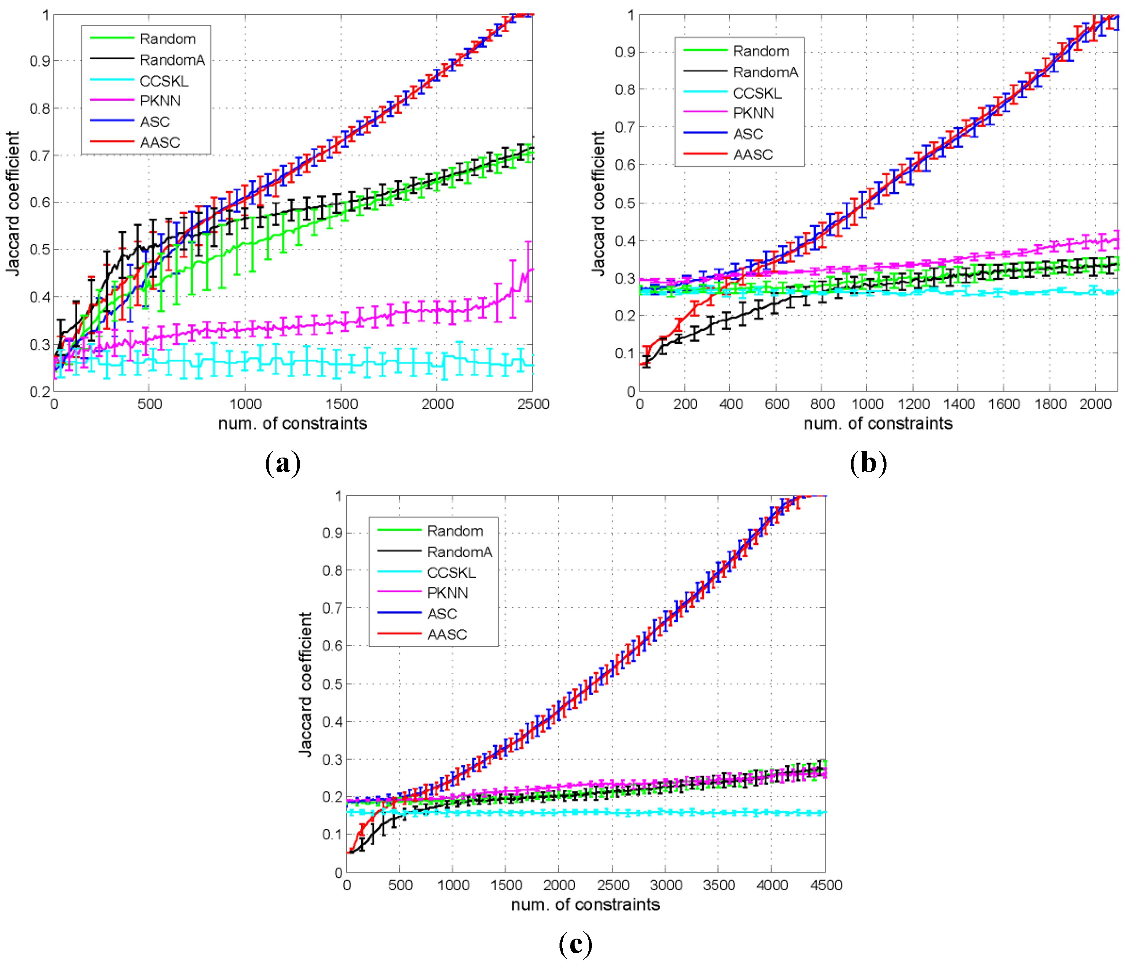
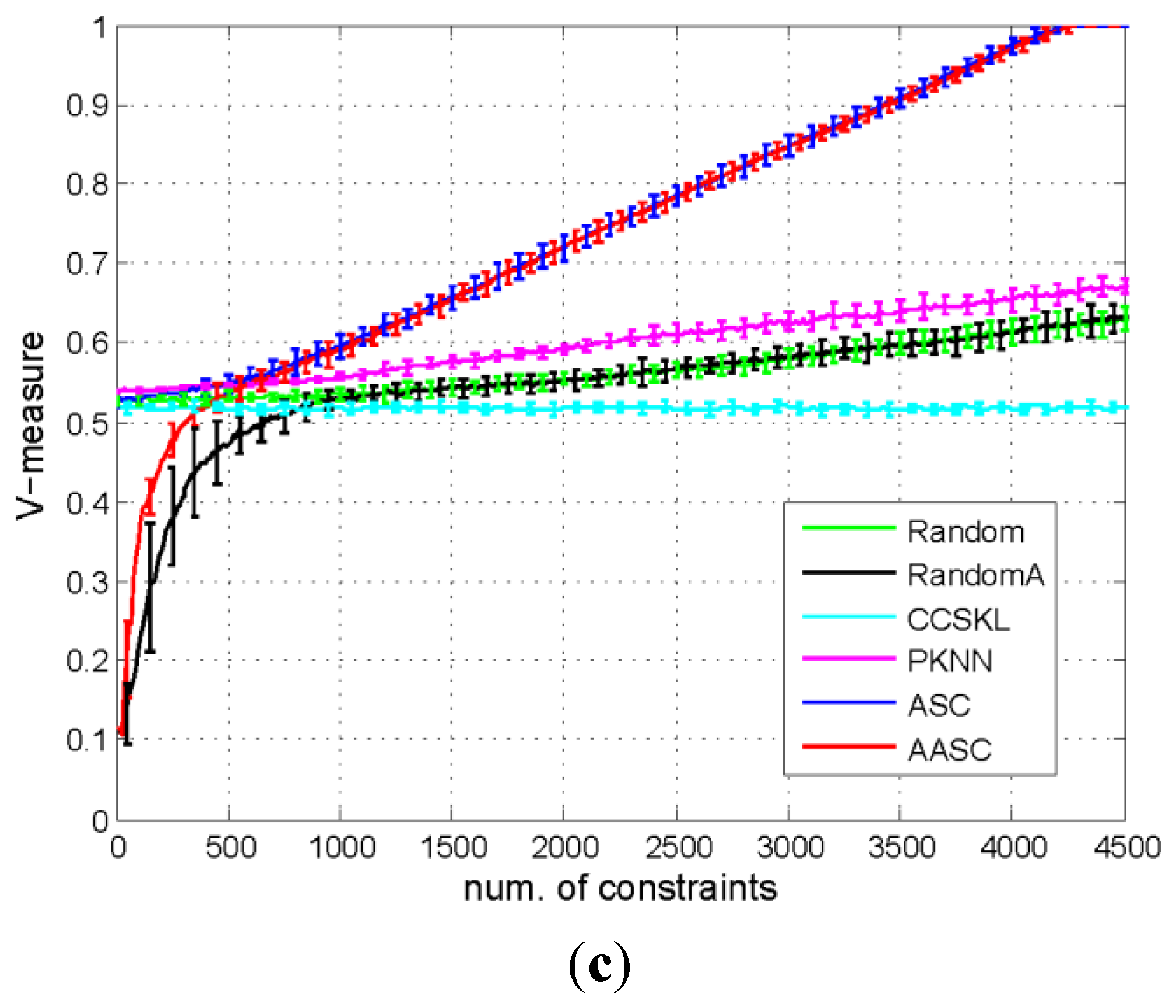
5.3.1. Comparison of the Performances of the Different Algorithms

In Figure 10 and Figure 11, we display the performances (mean accuracies and standard deviations in 50 runs) of the various algorithms on the three considered remote sensing image datasets, with an increasing number of questions posed to the oracles. To reach our target, a good annotation algorithm should yield a high mean accuracy with a small number of questions. Both the proposed ASC and AASC algorithms demonstrate superior performance compared with the state-of-the-art algorithms, and their standard deviations in accuracy are small and stable, indicating robust performance.
Figure 10. Clustering accuracy as evaluated using the V-measure. We ran each algorithm 50 times, and the results are shown as the means and standard deviations of the V-measure: (a) Beijing; (b) WHU-RS; and (c) UCM.
Remotesensing 07 15014 g010aRemotesensing 07 15014 g010b
Figure 11. Clustering accuracy as evaluated using the Jaccard coefficient. We ran each algorithm 50 times, and the results are shown as the means and standard deviations of the Jaccard coefficient: (a) Beijing; (b) WHU-RS; and (c) UCM.
Remotesensing 07 15014 g011
Both evaluation measures, the Jaccard coefficient and the V-measure, yield similar results on all datasets.
As a baseline algorithm, Random uses the same framework as ASC but randomly selects constraints from the current graph. A comparison of Random and CCSKL, both of which are two semi-supervised spectral clustering algorithms with random constraints, reveals that Random performs much better than CCSKL on the three datasets. From Figure 10 and Figure 11, it is evident that although the ASC algorithm outperforms the others, the proposed k-NN graph purification procedure is still effective even without active learning, which implies that the Random method can also be regarded as a reasonably effective semi-supervised clustering technique.
Figure 12 illustrates how the ASC algorithm purifies a k-NN graph through iterative purifications by displaying the similarity matrices for each dataset. Note that on all three datasets, with a greater number of active iterations (i.e., more queries of the oracle), the similarity matrices become increasingly discriminative. This finding confirms the efficiency and necessity of the active selection procedure in our proposed methods.
Figure 12. Evaluations of the similarity matrix with the iterative purification of the k-NN graph. From left to right: the similarity matrices after 1, 100, 240 and 500 iterations. From top to bottom: the similarity matrices for the Geo-eye image of Beijing, the WHU-RS dataset, and the UCM dataset. With an increasing number of iterations, the similarity matrices become increasingly discriminative.
Remotesensing 07 15014 g012
A comparison of the Random method and the proposed ASC algorithm reveals that the active selection step of ASC significantly improves the accuracy of the clustering results. This again demonstrates that active constraints are useful in semi-supervised clustering. With our proposed active learning step (more specifically, the node-uncertainty-based active select strategy), more useful and informative constraints can be selected to assist in spectral clustering. Therefore, to achieve a given accuracy, the human annotator is required to annotate fewer pairwise constraints, each of which represents an easier assignment task than the class-by-class annotation of remote sensing images. In Figure 10b and Figure 11b, it appears that Random performs equally well as or better than ASC in the early stage. This may be explained based on two considerations. First, our active strategy is dependent on the clustering results. Because of the large intra-class variance and small inter-class variance in the Beijing dataset, the feature description may not be sufficiently discriminative, yielding an imprecise clustering result and, in turn, leading to imprecise constraint selection. However, ASC considerably outperforms Random in later iterations with better clustering results. Second, the V-measure is more robust than the Jaccard coefficient, and the performance measured by the V-measure is more acceptable.
Figure 13. Change in the number of classes changes with an increasing number of constraints in AASC: (a) Beijing; (b) WHU-RS; and (c) UCM.
Remotesensing 07 15014 g013
Note that AASC runs without a given number of clusters, whereas the other algorithms require this number to be specified. Thus, for a fair comparison, RandomA was designed to use the same framework as AASC with the exception of the active selection step. By comparing AASC with RandomA, we can again reach a similar conclusion to that described above.
Note that the AASC algorithm also achieves comparable performance to the ASC algorithm, although the real number of clusters is not given as an input parameter. The question–accuracy curves of AASC are shown in Figure 10 and Figure 11. In early iterations, the performance of AASC is inferior to that of ASC because it performs spectral clustering with an unsuitable number of clusters m. However, in later iterations, as more different clusters are identified in the “Collect” step and m is updated to match the size of the set S, this value gradually approaches the real number of clusters (see Figure 13). With this tuning of the m value, the performance of AASC improves rapidly. In all of the experiments presented above, AASC is able to determine the real number of clusters within a reasonably small number of iterations. In the task of annotating remote sensing images, the AASC algorithm is more convenient for practical purposes because it does not require the number of clusters to be specified before the task is performed.
To more clearly explain the effectiveness of the ASC and AASC algorithms, Table 1 collects data regarding the actual constraints required to achieve completely correct annotations. Note that pairwise constraints represent a weaker form of supervised knowledge that contains less information and is easier to obtain than class labels. When we wish to obtain a completely correct annotation, it is necessary to assign class labels to 100% of the data. By contrast, in ASC and AASC, only a small portion (<0.4%) of the total pairwise constraints is required.
Table 1. Final numbers of constraints for ASC and AASC.
Dataset#Samples/#PairsASCAASC
#ConstraintsRatio#ConstraintsRatio
Beijing1600/127920023800.19%23520.18%
WHU-RS1063/56445319660.35%20420.36%
UCM2100/220395042390.19%42600.19%
The oracle querying component is key to allowing our proposed algorithms to operate in an online manner. To function properly, the algorithm should be fast enough that the human annotator is not required to wait a long time between two adjacent operations. Although some of the state-of-the-art methods tested above are also reasonably fast, more iterations are needed because of the low efficiency of their use of pairwise constraints. Among them, HACC is a recently proposed active clustering algorithm [37] that also actively seeks pairs, although in this case, the search is performed based on the expected change in the results. However, it is difficult to implement the HACC algorithm on our datasets because of its high time complexity, as shown in Table 2. Thus, to compare the performances of HACC and our proposed algorithm, we designed several sub-datasets via sampling from the UCM dataset, as shown in Table 3, and the corresponding results are presented in Table 2.
Table 2 shows that HACC can achieve efficiency in the use of pairwise constraints that is equal to that of ASC. However, ASC is greatly superior in terms of the time cost for each constraint.
Table 2. Results achieved on sub-datasets.
Dataset#ConstraintsTime (Total/Each )
HACCASCHACCASC
UCM-5-106257108 s/1.7 s0.6 s/0.01 s
UCM-5-2016815726 min/9.2 s0.9 s/5 ms
UCM-10-1030527750 min/9.84 s1.2 s/4.9 ms
UCM-10-2055344144 h/286 s2.44 s/5.5 ms
UCM-21-1010341019142 h/494 s4.68 s/4.6 ms
UCM-4239-231 s/0.05 s
Beijing-2380-175 s/0.07 s
WHU-RS-1966-39 s/0.02 s
Table 3. Sub-dataset specifications.
Dataset#Classes#Samples for each class#Total
UCM-5-1051050
UCM-5-20520100
UCM-10-101010100
UCM-10-201020200
UCM-21-102110210

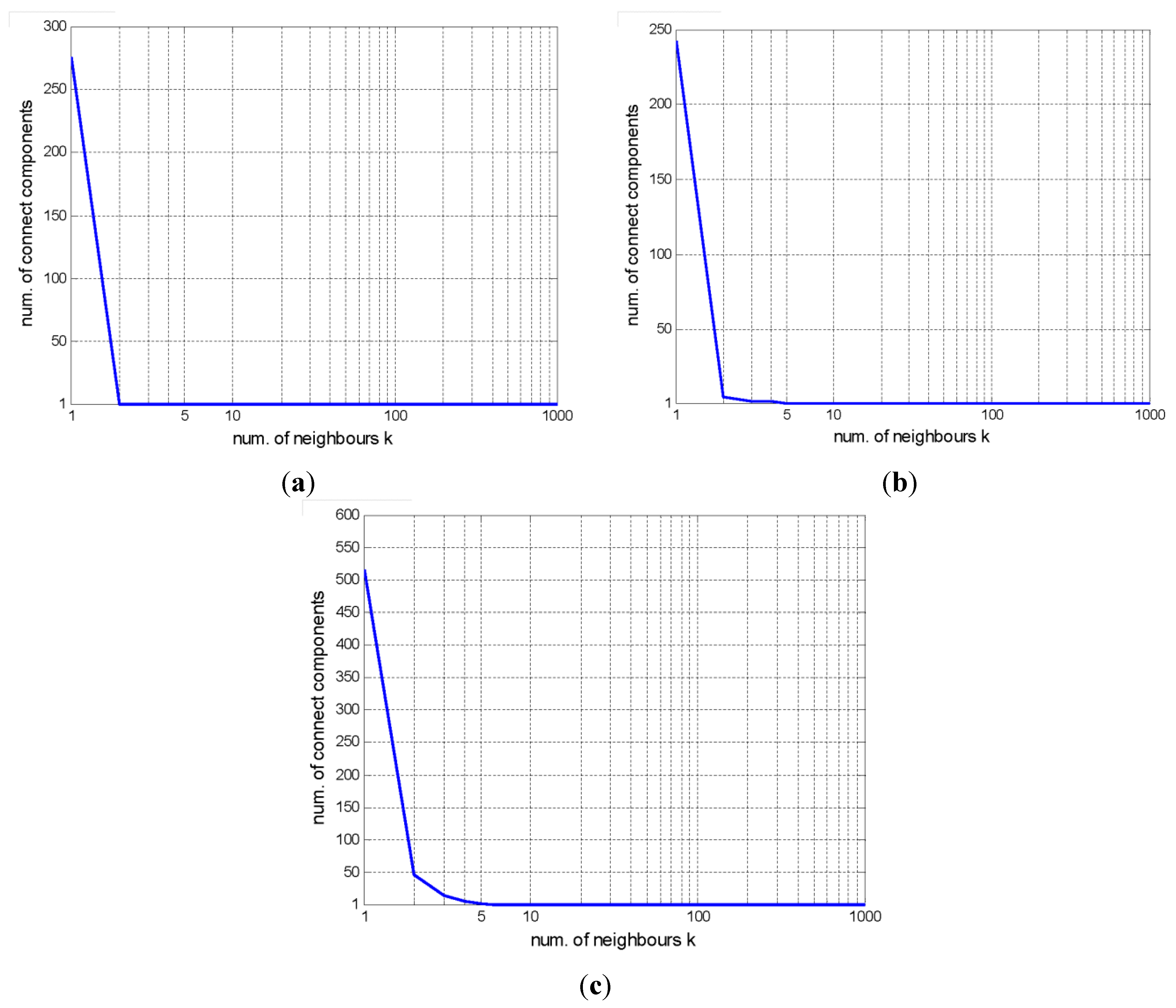
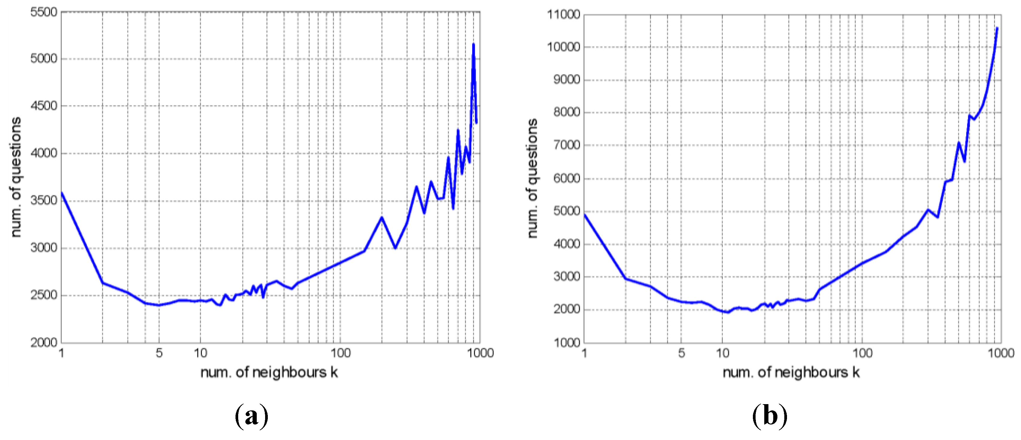
5.3.2. Effect of the Number of Neighbors k

Figure 14 illustrates how the parameter k of the k-NN graph affects ASC performance. Recalling the construction of the k-NN graph, it is clear that k is a critical parameter, as it determines how many edges are retained from the fully connected graph. As k increases, the neighborhood of each vertex become more global, meaning that more “abnormal neighbors” may appear and that the k-NN graph may be farther from perfect. Thus, as seen in Figure 14, ASC requires many more queries to achieve the same performance as k increases. By contrast, if k is too small (e.g., 1), the k-NN graph becomes a collection of hundreds of connected components instead of a connected graph, as seen in Figure 15. In that case, ASC cannot perform reasonably because of the lack of a merging strategy in the spectral clustering procedure, which is based on graph cut theory. Hence, the optimal choice is the smallest k for which the k-NN graph is a connected graph, or slightly larger. Based on these preliminary tests, we chose k = 10 for our experiments.
Figure 14. The effect of k on the initial k-NN graph. The curve shows the final number of queries for ASC as a function of k in the range of (1,1000): (a) Beijing; (b) WHU-RS; and (c) UCM.
Remotesensing 07 15014 g014aRemotesensing 07 15014 g014b
Figure 15. The number of connected components in the k-NN graph for different values of k. The curve shows the number of connected components in the k-NN graph as a function of k in the range of (1, 1000): (a) Beijing; (b) WHU-RS; and (c) UCM.
Remotesensing 07 15014 g015

5.3.3. Scene Annotation Results for Remote Sensing Images

In this section, we compare the performance of our algorithms with those of three recently proposed methods: the spectral clustering (SC) algorithm [45], the semi-supervised spectral clustering (S3C) algorithm [58] and the M3DA-RF algorithm [17], a recently proposed fully supervised method for the annotation task. Note that instead of actively collecting pairwise constraints, S3C performs spectral clustering using pairwise constraints provided prior to the clustering. The M3DA-RF algorithm is fully supervised and requires data labeled by experts as a training sample. To ensure a fair comparison, we used the same number of pairwise constraints for the S3C algorithm. To evaluate the performance of the clustering algorithms (as for supervised algorithms, e.g., M3DA-RF), the clustering accuracy was computed by assigning the label of each cluster to its closest class in the ground truth.
Figure 16. Comparison of the results of different methods for the annotation of a GeoEye-1 image of Beijing (refer to the text for more details): (a) original image; (b) human-labeled ground truth; (c) annotated via spectral clustering (SC) [45] (35.8%); (d) annotated via S3C [58]. (semi-supervised) (61.8%); (e) annotated via M3DA-RF [17] (fully supervised) (91.6%); and (f) annotated via AASC (99.2%).
Remotesensing 07 15014 g016
Figure 16 displays a comparison of our method with the three approaches mentioned above, namely, SC, S3C and M3DA-RF, when applied for the annotation of a large high-resolution satellite image, a GeoEye-1 image of Beijing. The M3DA-RF algorithm uses half of the labeled data as training samples and applies multi-level max-margin discriminative random field analysis for annotation. Note that M3DA-RF identifies spatial constraints via a conditional random field to improve its performance. From Figure 16, it is evident that S3C yields a far superior result (61.8%) to that of SC (35.8%), which suggests that pairwise constraints are very helpful for this task. The M3DA-RF algorithm, in turn, produces a better result (91.6%) than that of S3C. This is primarily because it uses training samples with class labels, which provide prior information that is much stronger than that offered by weak pairwise constraints. However, our method outperforms all three methods, yielding a nearly perfect annotation result (99.2%). Moreover, for AASC, we need not specify the number of clusters to be used in the clustering process. These results serve as the ultimate confirmation of our intuition regarding the proposed method, namely, that the weak prior knowledge provided by actively selected pairwise constraints can provide considerable guidance for the clustering algorithm.

6. Discussion

In this work, we have attempted to address the task of annotating remote sensing images with active clustering while reducing the manual cost using two different approaches. On the one hand, active learning is used to select efficient sample pairs to lighten the human workload in quantitative terms; on the other hand, as our supervised information, we use pairwise constraints, which are simpler than the traditional class labels assigned by experts.
Suitability of pairwise constraints for real problems: Because there are few methods that use pairwise constraints as supervised information for remote sensing image annotation, it is natural to question the suitability of using pairwise constraints for real problems. Consider the following facts: (1) First, the performance of the proposed method on several remote sensing image databases has demonstrated its efficacy for the task of remote sensing image annotation. (2) Although, as seen from the experimental results summarized in Table 1, it seems that ASC requires a large number of queries (even exceeding the size of the corresponding dataset) to complete the annotation task, it should be noted that we are attempting to use little or even non-expert knowledge for annotation. Obviously, pairwise constraints provide much weaker supervised information than that of class labels provided by an expert, not only because pairwise constraints are extremely easy to obtain simply by comparing two samples but also because they can be provided by human oracles with much less expert knowledge regarding the scene data. (3) A fair comparison of the required number of queries between pairwise constraints and class-label constraints should be based on the same level of expertise. For example, when a human oracle is asked to label an image sample in the UCM dataset using class labels, a method of doing so that is comparable to the use of pairwise constraints is as follows: he/she has knowledge of 21 pre-specified reference classes and compares the sample to each of these 21 classes to determine the appropriate label. For the UCM dataset (2100 images), this method of class labeling would require 21 × 2100 = 44,100 queries to complete the fully perfect annotation of the image, which is a much larger number than is required when using pairwise constraints (approximately 4000, or more than 10 times fewer). Thus, the number of queries required by our proposed algorithms is reasonably small.
In fact, when assigning a sample a label, the annotator needs to compare it with all of the reference classes, either in his/her mind or using actual images. Thus, the annotator must have a thorough understanding of all of the classes. By contrast, in the case of pairwise constraints, both images simultaneously serve as both test and reference images.
Moreover, even when implemented using a personal PC with a single-thread CPU, our method is fast and can operate in real time for interactive annotation. We can further speed up the algorithm by using parallel programming and querying multiple oracles.
Improvement of the annotation performance by means of better image descriptions: In the experiments presented in Section 5, bag-of-SIFT and bag-of-color descriptors were used to describe the remote sensing images. An unsupervised method yields clustering results that primarily depend on the descriptive capability of the features used. Indeed, better image descriptions may reduce the necessary number of queries. Here, we consider the use of promising features extracted using the CNN approach [59]. More precisely, each remote sensing image is described in terms of 4096 dimensional activations from the first fully connected layer. Then, the similarity between any two images is measured using a radial basis function (RBF) kernel, which can later be used to construct the k-NN graph. The performances of ASC and AASC using different types of features are presented in Figure 17. The number of queries is significantly reduced when we use CNN features.
Performance on larger and more complex datasets: It is also interesting to investigate the stability of the proposed algorithm with the scaling of the number of categories. To this end, we combined the WHU-RS and UCM datasets to construct a mixed dataset with 3163 samples. This dataset contains 31 classes, of which only 10 are common to both the WHU-RS and UCM datasets. Thus, the new mixed dataset is more challenging in terms of both the number of samples and the number of categories. Note that the sizes and the sources of the samples in these datasets are different, meaning that the intra-class variance is large, although the inter-class variance between samples from the same original dataset may be small. To describe the similarities between samples of different sizes, we use CNN features and compute the similarities using the RBF kernel. The results are displayed in Figure 18. When applied to this larger and more complex dataset, both the ASC and AASC algorithms still achieve a reasonable performance. Compared with the performances of the proposed methods and the PKNN algorithm presented in Figure 10 and Figure 11, the number of constraints is proportional to the size of the dataset for an equal accuracy improvement for our methods, whereas the PKNN shows less improvement with the same ratio of the number of constraints. Thus, the proposed methods are robust to the scaling of the number of categories.
Figure 17. Comparison of performance using different similarity measures. The number of constraints decreases when better features are used: (a) WHU-RS and (b) UCM.
Remotesensing 07 15014 g017
Figure 18. Results obtained on the mixed UCM and WHU-RS dataset. The results are shown as the means and standard deviations of the V-measure and the Jaccard coefficient: (a) V-measure and (b) Jaccard coefficient.
Remotesensing 07 15014 g018

7. Conclusions

In this paper, we address the problem of annotating remote sensing images via active clustering. Our method actively queries an oracle to obtain weak pairwise constraints. The proposed method uses node uncertainty as the active selection criterion, which offers improved accuracy in the selection of useful queries because more edges are considered per node. Thus, with an acceptable number of pairwise constraints, the clustering results show notable improvements. Moreover, we propose an improved algorithm that can adaptively determine the number of clusters during annotation. This is a very powerful capability in the classification of remote sensing images when there is no available prior knowledge (labeled training data, specific number and contents of categories) or when such information is difficult to acquire. From our experiment results, we can see that the proposed method is very suitable for mining meaningful scene clusters for the interpretation of remote sensing images. Our future research will include revising the similarity measure to obtain a more semantic similarity matrix during the running of the algorithm, using approaches such as metric learning techniques.

Acknowledgments

This research was supported by the National Natural Science Foundation of China under grants No. 91338113 and No. 41501462, and was partially funded by the Wuhan Municipal Science and Technology Bureau, with Chen-Guang Grant 2015070404010182.

Author Contributions

Gui-Song Xia conceived the original idea for the study and contributed to the article's organization. Zifeng Wang contributed to the implementation of the research. Caiming Xiong and Liangpei Zhang contributed to the discussion of the study design. Gui-Song Xia drafted the manuscript, which was revised by all authors. All authors read and approved the submitted manuscript.

Conflicts of Interest

The authors declare no conflict of interest.

References

  1. Tuia, D.; Camps-Valls, G. Recent advances in remote sensing image processing. In Proceedings of International Conference on Image Processing, Cairo, Egypt, 7–10 November 2009; pp. 3705–3708.
  2. Richards, J.A. Remote Sensing Digital Image Analysis; Springer: Berlin, Germany, 1999; Volume 3. [Google Scholar]
  3. Li, D.; Zhang, L.; Xia, G.-S. Automatic analysis and mining of remote sensing big data. Acta Geod. Cartogr. Sin. 2014, 43, 1211–1216. [Google Scholar]
  4. Wang, F. Fuzzy supervised classification of remote sensing images. IEEE Trans. Geos. Remote Sens. 1990, 28, 194–201. [Google Scholar] [CrossRef]
  5. Bandyopadhyay, S.; Maulik, U.; Mukhopadhyay, A. Multiobjective genetic clustering for pixel classification in remote sensing imagery. IEEE Trans. Geos. Remote Sens. 2007, 45, 1506–1511. [Google Scholar] [CrossRef]
  6. Mountrakis, G.; Im, J.; Ogole, C. Support vector machines in remote sensing: A review. ISPRS J. Photogramm. Remote Sens. 2011, 66, 247–259. [Google Scholar] [CrossRef]
  7. Aksoy, S.; Koperski, K.; Tusk, C.; Marchisio, G.; Tilton, J.C. Learning Bayesian classifiers for scene classification with a visual grammar. IEEE Trans. Geos. Remote Sens. 2005, 43, 581–589. [Google Scholar] [CrossRef]
  8. Friedl, M.; Brodley, C. Decision tree classification of land cover from remotely sensed data. Remote Sens. Environ. 1997, 61, 399–409. [Google Scholar] [CrossRef]
  9. Han, M.; Zhu, X.; Yao, W. Remote sensing image classification based on neural network ensemble algorithm. Neurocomputing 2012, 78, 133–138. [Google Scholar] [CrossRef]
  10. Xu, Y.; Huang, B. Spatial and temporal classification of synthetic satellite imagery: Land cover mapping and accuracy validation. Geosp. Inf. Sci. 2014, 17, 1–7. [Google Scholar] [CrossRef]
  11. Bruzzone, L.; Persello, C. A novel context-sensitive semisupervised SVM classifier robust to mislabeled training samples. IEEE Trans. Geos. Remote Sens. 2009, 47, 2142–2154. [Google Scholar] [CrossRef]
  12. Ruiz, P.; Mateos, J.; Camps-Valls, G.; Molina, R.; Katsaggelos, A.K. Bayesian active remote sensing image classification. IEEE Trans. Geos. Remote Sens. 2014, 52, 2186–2196. [Google Scholar] [CrossRef]
  13. Munoz-Mari, J.; Tuia, D.; Camps-Valls, G. Semisupervised classification of remote sensing images with active queries. IEEE Trans. Geos. Remote Sens. 2012, 50, 3751–3763. [Google Scholar] [CrossRef]
  14. Davidson, I.; Wagstaff, K.; Basu, S. Measuring Constraint-Set Utility for Partitional Clustering Algorithms; Springer Berlin Heidelberg: Berlin, Germany, 2006; pp. 115–126. [Google Scholar]
  15. Settles, B. Active Learning. Synthesis Lectures on Artificial Intelligence and Machine Learning; Morgan and Clay Pool: Long Island, NY, USA, 2012; Volume 6, pp. 1–114. [Google Scholar]
  16. Wang, Z.; Xia, G.-S.; Xiong, C.; Zhang, L. Spectral active clustering of remote sensing images. In Proceedings of IEEE Geoscience and Remote Sensing Symposium, Quebec, QC, Canada, 13–18 July 2014; pp. 1737–1740.
  17. Hu, F.; Yang, W.; Chen, J.; Sun, H. Tile-level annotation of satellite images using multi-level max-margin discriminative random field. Remote Sens. 2013, 5, 2275–2291. [Google Scholar] [CrossRef]
  18. Yang, W.; Yin, X.; Xia, G.-S. Learning high-level features for satellite image classification with limited labeled samples. IEEE Trans. Geos. Remote Sens. 2015, 53, 4472–4482. [Google Scholar] [CrossRef]
  19. Hu, F.; Xia, G.-S.; Wang, Z.; Huang, X.; Zhang, L.; Sun, H. Unsupervised feature learning via spectral clustering of multidimensional patches for remotely sensed scene classification. IEEE J. Sel. Top. Appl. Earth Obs. Remote Sens. 2015, 8, 2015–2030. [Google Scholar] [CrossRef]
  20. Liénou, M.; Maître, H.; Datcu, M. Semantic annotation of satellite images using latent Dirichlet allocation. IEEE Geos. Remote Sens. Lett. 2010, 7, 28–32. [Google Scholar] [CrossRef]
  21. Zhong, Y.; Zhang, L.; Gong, W. Unsupervised remote sensing image classification using an artificial immune network. Int. J. Remote Sens. 2011, 32, 5461–5483. [Google Scholar] [CrossRef]
  22. Hu, F.; Wang, Z.; Xia, G.-S.; Zhang, L. Fast binary coding for satellite image scene classification. In Proceedings of IEEE Geoscience and Remote Sensing Symposium, Milan, Italy, 26–31 July 2015.
  23. Foody, G.M.; Mathur, A.; Sanchez-Hernandez, C.; Boyd, D.S. Training set size requirements for the classification of a specific class. Remote Sens. Environ. 2006, 104, 1–14. [Google Scholar] [CrossRef]
  24. Tuia, D.; Volpi, M.; Copa, L.; Kanevski, M.; Munoz-Mari, J. A survey of active learning algorithms for supervised remote sensing image classification. IEEE J. Sel. Top. Signal Proces. 2011, 5, 606–617. [Google Scholar] [CrossRef]
  25. Shi, Q.; Du, B.; Zhang, L. Spatial coherence-based batch-mode active learning for remote sensing image classification. IEEE Trans. Image Proces. 2015, 24, 2037–2050. [Google Scholar] [CrossRef] [PubMed]
  26. Xu, J.; Hang, R.; Liu, Q. Patch-based active learning (PtAl) for spectral-spatial classification on hyperspectral data. Int. J. Remote Sens. 2014, 35, 1846–1875. [Google Scholar] [CrossRef]
  27. Tuia, D.; Kanevski, M.; Marí, J.M.; Camps-Valls, G. Cluster-based active learning for compact image classification. In Proceedings of the IEEE International Geoscience and Remote Sensing Symposium, Honolulu, HI, USA, 25–30 July 2010; pp. 2824–2827.
  28. Demir, B.; Bovolo, F.; Bruzzone, L. Detection of land-cover transitions in multitemporal remote sensing images with active-learning-based compound classification. IEEE Trans. Geos. Remote Sens. 2012, 50, 1930–1941. [Google Scholar] [CrossRef]
  29. Tuia, D.; Munoz-Mari, J.; Camps-Valls, G. Remote sensing image segmentation by active queries. Pattern Recogn. 2012, 45, 2180–2192. [Google Scholar] [CrossRef]
  30. Demir, B.; Bruzzone, L. A novel active learning method in relevance feedback for content-based remote sensing image retrieval. IEEE Trans. Geos. Remote Sens. 2015, 53, 2323–2334. [Google Scholar] [CrossRef]
  31. Taheri, S.H.; Bagheri, S.S.; Fell, F.; Schaale, M.; Fischer, J.; Tavakoli, A.; Preusker, R.; Tajrishy, M.; Vatandoust, M.; Khodaparast, H. Application of the active learning method to the retrieval of pigment from spectral remote sensing reflectance data. Int. J. Remote Sens. 2009, 30, 1045–1065. [Google Scholar] [CrossRef]
  32. Demir, B.; Persello, C.; Bruzzone, L. Batch-mode active-learning methods for the interactive classification of remote sensing images. IEEE Trans. Geos. Remote Sens. 2011, 49, 1014–1031. [Google Scholar] [CrossRef]
  33. Sun, S.J.; Zhong, P.; Xiao, H.T.; Wang, R.S. Active learning with Gaussian process classifier for hyperspectral image classification. IEEE Trans. Geos. Remote Sens. 2015, 53, 1746–1760. [Google Scholar] [CrossRef]
  34. Tuia, D.; Ratle, F.; Pacifici, F.; Kanevski, M.F.; Emery, W.J. Active learning methods for remote sensing image classification. IEEE Trans. Geos. Remote Sens. 2009, 47, 2218–2232. [Google Scholar] [CrossRef]
  35. Xiong, C.; Johnson, D.; Corso, J.J. Spectral active clustering via purification of the k-nearest neighbor graph. In Proceedings of European Conference on Data Mining, Lisbon, Portugal, 21–23 July 2012.
  36. Mallapragada, P.K.; Jin, R.; Jain, A.K. Active query selection for semi-supervised clustering. In Proceedings of the 19th International Conference on Pattern Recognition, Tampa, FL, USA, 8–11 December 2008; pp. 1–4.
  37. Biswas, A.; Jacobs, D. Active image clustering with pairwise constraints from humans. Int. J. Comput. Vis. 2014, 108, 133–147. [Google Scholar] [CrossRef]
  38. Xu, Q.; Desjardins, M.; Wagstaff, K.L. Active constrained clustering by examining spectral eigenvectors. In Proceedings of the 8th International Conference on Discovery Science, Singapore, 8–11 October 2005; pp. 294–307.
  39. Wang, X.; Davidson, I. Active spectral clustering. In Proceedings of IEEE 10th International Conference on Data Mining, Sydney, Australia, 14–17 December 2010; pp. 561–568.
  40. Wagstaff, K.; Cardie, C. Clustering with Instance-Level Constraints. In Proceedings of AAAI-00, Austin, TX, USA, 30 July–3 August 2000; pp. 1097–1097.
  41. Klein, D.; Kamvar, S.D.; Manning, C.D. From instance-level constraints to space-level constraints: Making the most of prior knowledge in data clustering. In Proceedings of the 19th International Conference on Machine Learning, Sydney, Australia, 8–12 July 2002.
  42. Basu, S.; Banerjee, A.; Mooney, R.J. Active semi-supervision for pairwise constrained clustering. In Proceedings of the 4th SIAM International Conference on Data Mining, Lake Buena Vista, FL, USA, 22–24 April 2004; pp. 333–334.
  43. Eriksson, B.; Dasarathy, G.; Singh, A.; Nowak, R.D. Active clustering: Robust and efficient hierarchical clustering using adaptively selected similarities. In Proceedings of International Conference on Artificial Intelligence and Statistics, Fort Lauderdale, FL, USA, 11–13 April 2011; pp. 260–268.
  44. Von Luxburg, U. A tutorial on spectral clustering. Stat. Comput. 2007, 17, 395–416. [Google Scholar] [CrossRef]
  45. Ng, A.Y.; Jordan, M.I.; Weiss, Y. On spectral clustering: Analysis and an algorithm. In Proceedings of NIPS, Vancouver, BC, Canada, 3–8 December 2001; pp. 849–856.
  46. Lowe, D. Distinctive image features from scale-invariant keypoints. Int. J. Comput. Vis. 2004, 60, 91–110. [Google Scholar] [CrossRef]
  47. Yang, Y.; Newsam, S. Bag-of-visual-words and spatial extensions for land-use classification. In Proceedings of 18th SIGSPATIAL International Conference on Advances in GIS, San Jose, CA, USA, 2–5 November 2010; pp. 270–279.
  48. Csurka, G.; Dance, C.; Fan, L.; Willamowski, J.; Bray, C. Visual categorization with bags of keypoints. workshop Stat. Learn. Comput. Vis. 2004, 1, 1–2. [Google Scholar]
  49. Xia, G.-S.; Delon, J.; Gousseau, Y. Accurate junction detection and characterization in natural images. Int. J. Comput. Vis. 2014, 106, 31–56. [Google Scholar] [CrossRef]
  50. Liu, G.; Xia, G.-S.; Huang, X.; Yang, W.; Zhang, L. A perception-inspired building index for automatic built-up area detection in high-resolution satellite images. In Proceedings of Geoscience and Remote Sensing Symposium, Melbourne, Australia, 21–26 July 2013; pp. 3132–3135.
  51. Xia, G.-S.; Delon, J.; Gousseau, Y. Shape-based invariant texture indexing. Int. J. Comput. Vis. 2010, 88, 382–403. [Google Scholar] [CrossRef]
  52. Liu, G.; Xia, G.-S.; Yang, W.; Zhang, L. Texture analysis with shape co-occurrence patterns. In Proceedings of International Conference on Pattern Recognition (ICPR), Stockholm, Sweden, 24–28 August 2014; pp. 1627–1632.
  53. Swain, M.J.; Ballard, D.H. Color indexing. Int. J. Comput. Vis. 1991, 7, 11–32. [Google Scholar] [CrossRef]
  54. Ting, D.; Huang, L.; Jordan, M. An analysis of the convergence of graph Laplacians. In Proceedings of the 27th International Conference on Machine Learning, Haifa, Israel, 21–24 June 2010.
  55. Xia, G.-S.; Yang, W.; Delon, J.; Gousseau, Y. Structural high-resolution satellite image indexing. In Proceedings of ISPRS TC VII Symposium–100 Years, Vienna, Austria, 5–7 July 2010; pp. 298–303.
  56. Tan, P.-N.; Steinbach, M.; Kumar, V. Introduction to Data Mining; Addison Wesley: Boston, MA, USA, 2006. [Google Scholar]
  57. Rosenberg, A.; Hirschberg, J. V-measure: A conditional entropy-based external cluster evaluation measure. EMNLP-CoNLL ACL 2007, 7, 410–420. [Google Scholar]
  58. Li, Z.; Liu, J. Constrained clustering by spectral kernel learning. In Proceedings of International Conference on Computer Vision, Kyoto, Japan, 29 September–2 October 2009; pp. 421–427.
  59. Jia, Y.; Shelhamer, E.; Donahue, J.; Karayev, S.; Long, J.; Girshick, R.; Guadarrama, S.; Darrell, T. Caffe: Convolutional architecture for fast feature embedding. In Proceedings of the ACM International Conference on Multimedia, Orlando, FL, USA, 3–7 November 2014; pp. 675–678.

