Article

A Comparative Study of Sampling Analysis in the Scene Classification of Optical High-Spatial Resolution Remote Sensing Imagery

1
State Key Laboratory for Information Engineering in Surveying, Mapping and Remote Sensing (LIESMARS), Wuhan 430079, China
2
Electronic Information School, Wuhan University, Wuhan 430072, China
*
Author to whom correspondence should be addressed.
Remote Sens. 2015, 7(11), 14988-15013; https://doi.org/10.3390/rs71114988
Submission received: 11 August 2015 / Revised: 27 October 2015 / Accepted: 3 November 2015 / Published: 10 November 2015

Abstract

:
Scene classification, which consists of assigning images with semantic labels by exploiting the local spatial arrangements and structural patterns inside tiled regions, is a key problem in the automatic interpretation of optical high-spatial resolution remote sensing imagery. Many state-of-the-art methods, e.g., the bag-of-visual-words model and its variants, the topic models and unsupervised feature learning-based approaches, share similar procedures: patch sampling, feature learning and classification. Patch sampling is the first and a key procedure, and it has a considerable influence on the results. In the literature, many different sampling strategies have been used, e.g., random sampling and saliency-based sampling. However, the sampling strategy that is most suitable for the scene classification of optical high-spatial resolution remote sensing images remains unclear. In this paper, we comparatively study the effects of different sampling strategies under the scenario of scene classification of optical high-spatial resolution remote sensing images. We divide the existing sampling methods into two types: random sampling and saliency-based sampling. Here, we consider the commonly-used grid sampling to be a specific type of random sampling method, and the saliency-based sampling consists of keypoint-based sampling and salient region-based sampling. To compare their performances, we rely on a standard bag-of-visual-words model to learn the global features for testing because of its simplicity, robustness and efficiency. In addition, we conduct experiments using a Fisher kernel framework to validate our conclusions. The experimental results obtained on two commonly-used datasets using different feature learning methods show that random sampling can provide comparable and even better performance than all of the saliency-based strategies.

Graphical Abstract

1. Introduction

Over the past decade, with the rapid development of remote sensing imaging techniques, a considerable amount of high-spatial resolution remote sensing (HSR-RS) images are now available, which enable us to measure the ground surface with high precision. Scene classification of optical HSR-RS imagery, which aims to classify extracted subregions of HSR-RS images covering multiple land cover types or ground objects into different semantic categories, has recently attracted considerable attention in remote sensing image interpretation [1,2,3,4,5,6,7,8,9,10,11,12,13,14,15,16,17].
By a “scene” in the context of interpreting HSR-RS images, this usually refers to local areas in images that contain clear semantic information on the surface, e.g., the residential area, commercial area, farmland, green land and bare land. Scene classification can provide an overall layout for HSR-RS images containing various types of complicated land covers and object-oriented scenes. In contrast with pixel-based and object-based classification approaches, which focus on classifying pixels or objects (groups of local homogeneous pixels) into their thematic classes by aggregating spectral, textural and geometrical features, scene classification aims to cross the barrier between low-level visual features and high-level semantic information to interpret optical HSR-RS imagery automatically, and it can be widely used for many applications, such as change detection, urban planning and environmental monitoring, among others.
Observe that, in order to do scene classification for a large-scale HSR-RS image, one often requires to first construct the basic scene elements for classification, by using either non-overlapping tiles [2,5,13], overlapping tiles [10,14,16] or super-pixels [4,11]. However, the core problem is how to establish the scene models, i.e., exploiting the variations in the local spatial arrangements and structural patterns inside local tiled regions. Thus, most of research focuses on studying tile-level scene classification under the simplest non-overlapping-tile setting [1,3,6,7,8,9,12,15,17], while leaving the problem of scene element extraction aside. This paper follows the same simple setting and concentrates on the scene modeling procedure.

1.1. Problem and Motivation

In recent years, numerous studies have been devoted to the scene classification of optical HSR-RS imagery; see, e.g., [1,2,3,4,5,6,7,8,9,10,11,12,13,14,15,16,17]. Although the methods of scene classification involve many different methodologies, such as the bag-of-visual-words (BoVW) models [1,4,9], the topic models [3,8] and unsupervised feature learning-based methods [10,13,14], it is clear that one can summarize these methods into three main components, namely patch sampling, feature learning and classification, each of which has a considerable influence on the final performance. In the literature, most works focus on the latter two different components, e.g., designing/learning efficient scene features and classifiers [2,4,7,8,9,10,12,13,14,15], while the influence of sampling strategies is underestimated, and thus, few works have been devoted to the sampling step. However, one should note the following facts:
-
Sampling is an essential step for the scene classification of optical HSR-RS imagery. In image analysis, sampling is concerned with the selection of a subset of pixels from an image to estimate characteristics of the entire image. It is essential primarily because the volume of image data is often too large to be processed, and a small yet representative set of data is demanded. For instance, without sampling, it is intractable or even infeasible to train a BoVW model or unsupervised feature learning-based model for scene classification [4,9,10,13,14] with a computer of advanced configurations, as the volume of optical HSR-RS imagery generally amounts to several gigabytes.
-
Sampling strategies are crucial to the performance of the scene classification of optical HSR-RS imagery. The main goal of sampling is to select a representative subset of the entire data. The subsequent procedures directly process the sampled data while leaving out the information of all of the unselected ones; thus, how to sample the image data containing the most descriptive and discriminative information for classification has a considerable influence on the final results. Good samples can guarantee the classification performance and simultaneously achieve substantial improvements in the time and space complexities, whereas non-representative samples will considerably reduce the performance. Thus, in scenarios of scene classification of optical HSR-RS imagery, it is crucial to pursue a sampling strategy that balances the classification accuracy and the space and time complexity. However, it is not yet clear how to choose suitable sampling strategies.
-
There is a lack of studies on sampling strategies for the scene classification of optical HSR-RS imagery. Note that different sampling strategies have been used by recent scene classification approaches, e.g., grid sampling by [1,10,14] and a saliency-based one in [13]. To our knowledge, however, there are few comparative studies between these strategies.
-
Sampling strategies in natural scenes cannot be copied to the scene classification of optical HSR-RS imagery. Note that sampling strategies have been better understood in natural images, e.g., some comparisons on sampling strategies have been made in natural image classification [18,19]. However, it cannot be copied to the scenarios of optical HSR-RS imagery, because there are large differences between them, e.g., in the shooting angles and occlusions. For instance, natural images are primarily captured by cameras in the front with manual focus and even auto-focus capabilities, and it thus makes the natural scenes tend to be upright and center biased, which is obviously not the case of remote sensing images that are often taken from overhead. Consequently, this makes the appearances of the scene quite different. Moreover, the definitions of the scene are different between natural images and optical HSR-RS images. For natural images, the scene is often classified into indoor and outdoor types [18,20,21]. However, for optical HSR-RS images, the indoor types do not exist, and the outdoor types are further classified into forest, desert, commercial area, residential area, and so on.
Thus, it is of great importance and interest to study the influence of the different sampling strategies on the scene classification of optical HSR-RS images to provide some instructions for later works when they need to choose a sampling strategy.

1.2. Objective and Contributions

To investigate and quantitatively compare different sampling strategies fairly, we fix the other two components, i.e., feature learning and classifier, of scene classification and primarily test the influence of sampling strategies for the sake of simplicity. More specifically, we choose the standard BoVW model to construct a unified feature learning scheme embedded with various sampling strategies and choose the support vector machine (SVM) classifier for classification. Although the BoVW model does not necessarily perform better than other state-of-the-art methods, it is very efficient, robust and easy to implement. Moreover, because the sampling step is an independent procedure, the comparison results achieved with the BoVW model under such a scheme can be extended to other methods. Thus, we have also conducted the experiments using a Fisher kernel approach [22] for feature learning to validate its expandability. We perform our experiments on two commonly-used datasets on the topic of scene classification in optical HSR-RS imagery.
Our work is distinguished by the following contributions:
-
Our work is the first to study and compare the effects of many different sampling strategies on the scene classification of optical HSR-RS imagery, which is in contrast with previous works that only choose a certain sampling strategy, but concentrate on developing discriminative feature descriptions or classifiers. Our results can be used to improve the performance of previous works while being very instructive for future works on the scene classification of optical HSR-RS imagery.
-
We have intensively studied the performances of various saliency-based sampling strategies that are recently proposed and highlighted to be useful for classification on different types of scenes. Our experiments show that saliency-based sampling is mainly helpful for object-centered scenes, but does not work for scenes with complex textures and geometries.
The remainder of this paper is organized as follows. In Section 2, we briefly introduce the related works on different sampling strategies. In Section 3, we describe our method for comparing different sampling strategies in detail. In Section 4, the datasets used in our experiment are presented. The experimental results are shown and analyzed in Section 5, and the last section presents the conclusions of our work.

2. Related Work

As previously mentioned, sampling is a key step for constructing an intelligent system for image classification or recognition. This section attempts to provide a brief review of the existing works on this topic.
The volume of remote sensing images, particularly optical HSR-RS images, is often too vast to be processed directly. A sampling step is typically required to select an informative and representative subset of the images for subsequent analysis. In the literature, various sampling strategies have been used in the processing of optical HSR-RS images [1,2,4,7,8,9,10,12,13,14]. For instance, to construct a BoVW model to achieve better performance in land use classification, Yang et al. [1] sampled the patches of images using a uniform grid and adapted the spatial pyramid match kernel method [23] by incorporating the relative spatial information rather than the absolute one. Recently, unsupervised feature learning-based methods have exhibited superiority in learning descriptive features for optical HSR-RS images [10], and many studies have been devoted to this direction, in which sampling is a crucial step. For example, Hu et al. [14] proposed the use of grid-sampled patches of images for unsupervised feature learning for scene classification, whereas Zhang et al. [13] used a context-aware saliency detection model to sample the salient regions. Although different sampling strategies have been used, few comparative studies of these sampling strategies have been performed, and how to efficiently use the various sampling strategies in the processing of optical HSR-RS images remains unclear.
In contrast with the case of remote sensing images, the sampling strategies have been widely investigated in the field of natural image processing. Grid sampling is the most widely-used approach because of its simplicity; see, e.g., [23,24,25,26], where patches are uniformly sampled in the spatial domain with a step (e.g., four pixels) in an image. With the development of various keypoint detectors [27,28,29], which have shown great abilities in finding interest points, some researchers have used them to sample the patches [30,31,32,33,34] containing the interest points, which are believed to be more informative and representative [30]. However, it has been proven that such keypoint detectors cannot improve the classification performance [35,36], because they were not designed for classification problems, but rather for image matching applications. Surprisingly, it has been found that random sampling, another sampling method, is often more discriminant than keypoint-based methods [18,19]. In recent years, some researchers have also used saliency detection [37,38,39], aiming at first sampling the patches that belong to the salient regions that are in accordance with human visual attention mechanism.
An early comparative study of the various sampling strategies in natural image classification was performed in [18], which found that grid sampling provided the best performance by using a Bayesian hierarchical model. In addition, Nowak et al. [19] compared the different sampling methods and concluded that random sampling outperforms the sophisticated multi-scale interest detectors with large numbers of sampled patches.
There is a lack of comparative studies on the sampling strategies for optical HSR-RS images, such as the work in [18,19] for natural images. Moreover, due to the large difference between optical HSR-RS images and natural images mentioned previously, one cannot directly borrow the conclusions from natural images to use for optical HSR-RS images. In addition, saliency detection [40,41,42,43] has recently become a hot topic in image analysis, and many works have used this as a sampling strategy, e.g., [13,37,38,39]. However, how to properly use these sampling methods to help the classification task remains a problem. This paper thus attempts to provide a comparative study of the various sampling strategies for the classification of optical HSR-RS images.

3. Method for the Comparative Study

This section describes the method for conducting the comparative study of different sampling strategies.

3.1. Scheme of the Comparative Study

To compare different sampling strategies in the case of the scene classification for optical HSR-RS images fairly, we keep the feature learning and classification fixed and only vary the sampling approaches in the entire procedure. For feature learning, we use the BoVW model because of its simplicity, robustness and efficiency. Moreover, we adopt another efficient feature learning model, the Fisher kernel, to validate the conclusions drawn from the BoVW model. Thus, the investigated sampling strategies and the conclusions are also applicable to other feature-learning approaches. For classification, we use the most widely-used SVM classifier. The flowchart of the comparative study scheme is presented in Figure 1, which consists of three main steps:
-
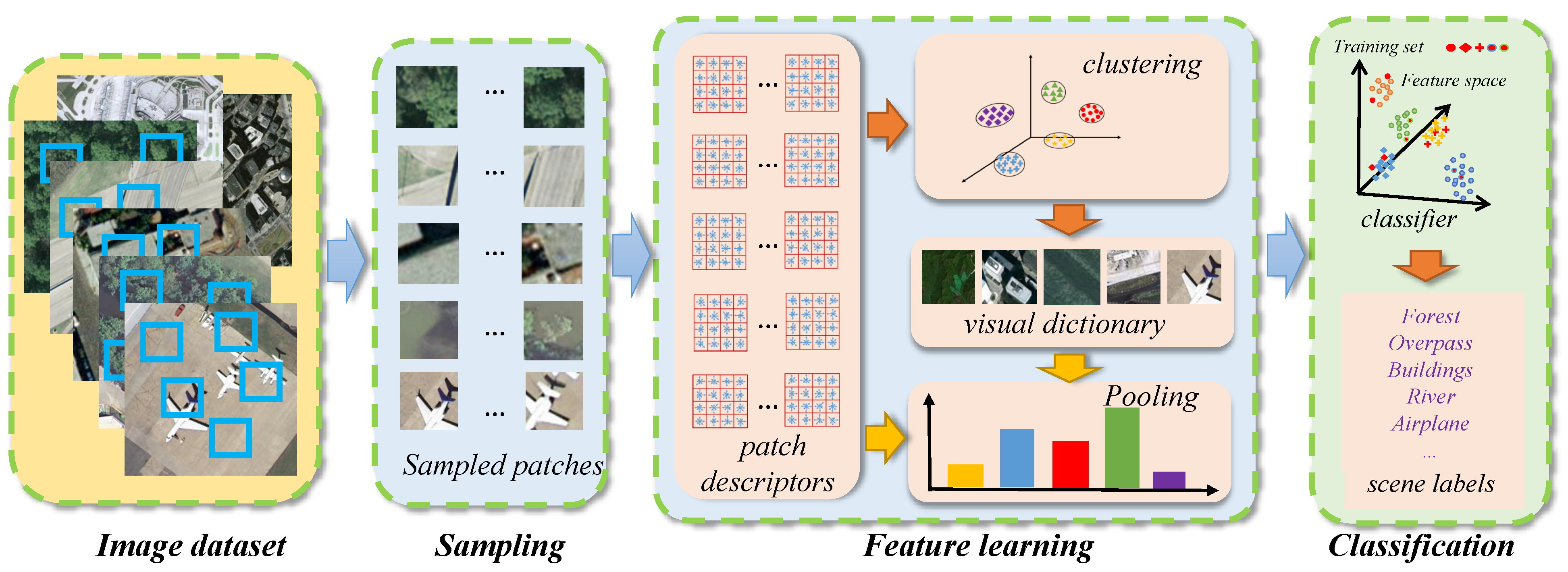
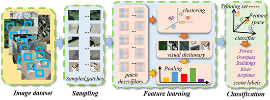
Sampling: selecting a compact, but representative subset of images. Given an image, a set of local image patches is selected via different sampling methods (e.g., random or saliency-based sampling strategies) to form a representative and informative subset of the image. Here, a patch is a local rectangular image region that can be used for feature description in the following step. Compared to the original image, the sampled subset of patches is more compact and has less space complexity. This step is the core part of our work, which the comparative studies are devoted to, and is illustrated in more detail in the following part.
-
Feature learning: learning feature descriptions of the images using sampled patches. Each patch in the sampled set is first characterized by certain feature descriptors, such as scale-invariant feature transform (SIFT) [28] or histogram of gradients (HoG) [44], or other texture [45,46] descriptors. In our work, we use the most popular SIFT descriptor as the patch descriptor because of its invariance and robustness. Thus, the size of a patch is set to be 16 × 16 pixels. By computing the histograms of gradient directions over a 4 × 4 spatial grid and quantizing the gradient directions into eight bins, the final SIFT descriptor of a patch has dimensions of 128 ( 4 × 4 × 8 ). Based on such a patch description, one can then learn a feature representation of the image, e.g., by using the BoVW model, topic models [8,47,48] or the recently-proposed unsupervised feature learning methods [10,13,14]. In our case, we use the BoVW for feature learning. More precisely, it first applies a k-means clustering algorithm to the descriptors of sampled patches to form a dictionary of visual words (with a size of K), and then, it uses hard assignment to quantify the descriptors of sampled patches against the dictionary to obtain a histogram-like global feature. In the experiment, K is empirically set to be 1000 for both datasets in k-means. The resulting K-dimension global feature vector is finally normalized as a characterization of an image. In addition, we adopt another feature learning method, the Fisher kernel [22], to validate the expandability of the conclusions drawn from the BoVW model. This model is a generic framework that combines the benefits of generative and discriminative approaches. It uses the Gaussian mixture model (GMM) to construct a visual word dictionary rather than k-means, and it describes an image using the Fisher vector-encoding method using mean and covariance deviation vectors. Because the Gaussian mixture model is adopted to fit every dimension of the local descriptors, for the adopted 128-dimensional SIFT descriptor, the dimension of the final image vector will be 256-times the dictionary size K. Thus, it can work well by using a considerably smaller dictionary size (e.g., K is empirically set to be 100 for both datasets in our work) than the BoVW model, and principle component analysis (PCA) is adopted for dimension reduction prior to classification.
-
Classification: assigning a semantic class label to each image. This step occurs after finding a feature representation of images and typically relies on some trained classifier, e.g., SVM. Because this part is beyond the scope of our study in this paper, in our experiments, we employ the commonly-used libSVM [49] as our classifier. For BoVW, we use the histogram intersection kernel [50], which is a very suitable non-linear kernel for measuring the similarity among histogram-based feature vectors. For the Fisher kernel, we adopt the radial basis function (RBF) kernel for its good performance. For both testing datasets, a unique ground truth label corresponding to every sample image exists. The labeling work is carefully performed by experts in this field. Therefore, the performances of supervised classification with different sampling methods are evaluated. Specifically, we randomly select a subset of images from the dataset for training to construct the classification model by SVM, and the remaining images are used for testing to measure the performance. This process is repeated 100 times, and the average classification accuracy and its standard deviation are computed. With the UC-Merced dataset, we randomly select 80 % of the samples from each class to train the classifier, which is a general setting in the literature, while for the RS19dataset, we randomly select 60 % for training.
Figure 1. Flowchart of the comparative study scheme. It consists of three main steps. Sampling is used to select a compact, but representative subset of images. Feature learning is to learn feature descriptions of the images using the sampled data. Classification is for assigning a semantic class label to each image. Here, the feature learning step is based on the bag-of-visual-words model and the Fisher kernel approach, but note that the studied sampling strategies and the entire procedure are also applicable to other feature learning approaches.
Remotesensing 07 14988 g001

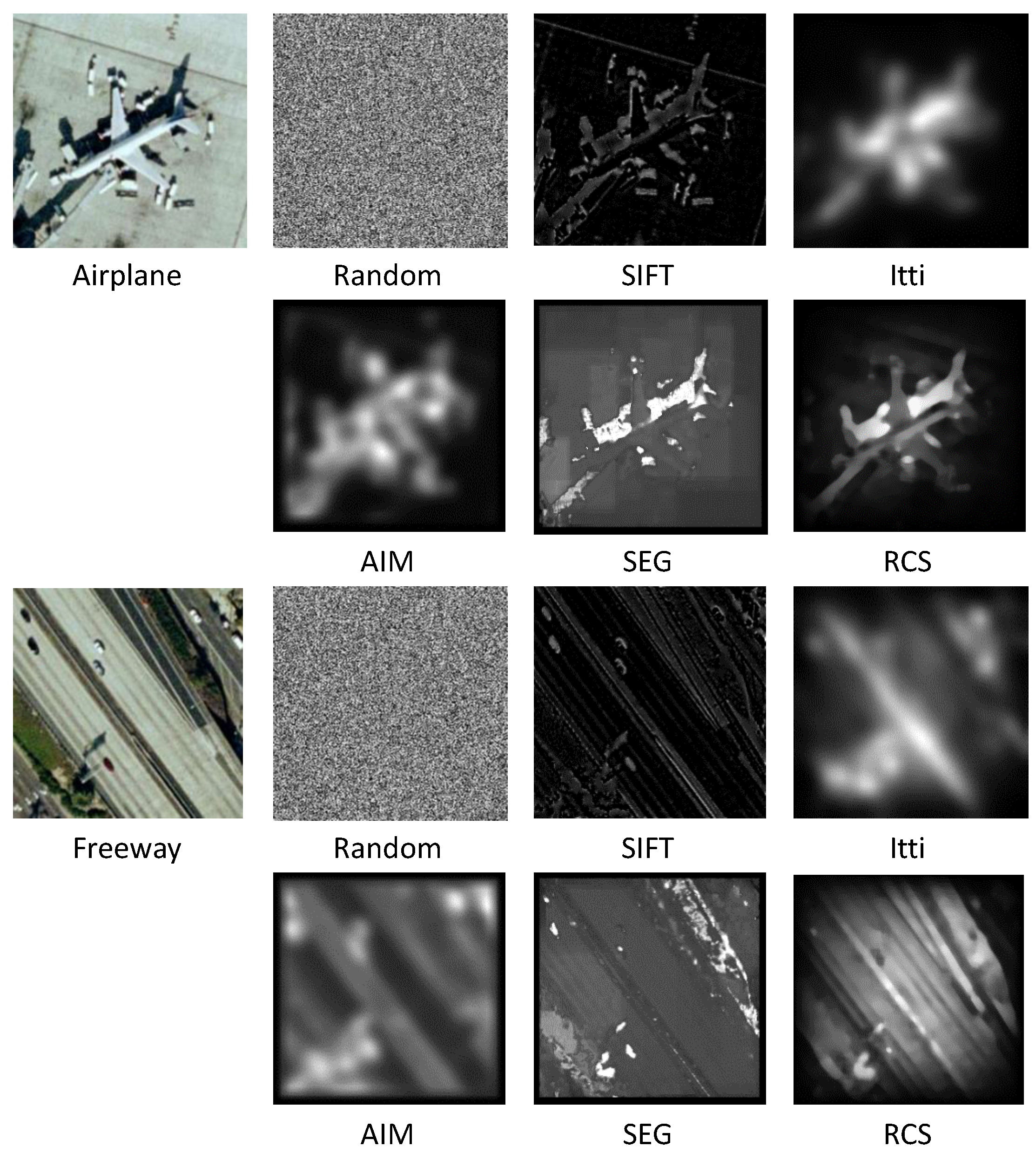
3.2. Involved Sampling Strategies

Given an image f : Ω R D , where Ω = { 0 , 1 , , M 1 } × { 0 , 1 , , N 1 } , M and Ndenote the number of rows and columns of an image, and D denotes the number of channels, e.g., D = 3 for RGB images in our work, define the sampling ratio r to be the number of sampled patches divided by the number of pixels in an image; sampling is to find a subset S of Ω for a given ratio r, such that:
S : = p | p Ω , f ( x ) is  i n f o r m a t i v e , # p M × N = r
where p represents a local rectangular image region centered at the image pixel x, f ( x ) is the response value computed by different sampling methods at x and # p denotes the number of patches.
We define the sampling ratio r to be the number of sampled patches divided by the number of pixels in an image. Thus, at the same sampling ratio, there are the same number of patches to be chosen to form the representative set for images of the same size. In our experiment, different sampling strategies are evaluated with the range of sampling ratios varying from 0 . 01 to 1, and the step is set to be 0 . 01 ; thus, r = 1 indicates grid sampling with the spacing set at 1 pixel.
Specifically, for different sampling strategies, we first produce its response map for a given image, and the response map then serves as a mask to sample the local patches according to the values in the mask: the patches centered at larger values are first sampled until the sampling ratio is equal to the given one.
The content of S depends on the definition of the term informative. For instance, if one takes the informative image content as the patches that contain key local feature points or image structures that are sufficiently salient in an image, then it corresponds to the saliency-based sampling. If one considers all of the patches to be equal, which means that every patch has the same probability to be sampled to represent the image content, then it indicates random sampling.
The sampling strategies adopted in this paper are illustrated in Table 1, and each of them will be reviewed in this section.
Table 1. Different sampling strategies investigated in this work.
Sampling StrategyMethod and Description
random Random: randomly sample local patches in the spatial domain
SIFT [28]: compute the DoG response map
Itti [40]: integrate color, intensity and orientation features across the scale to generate the saliency map
saliency basedAIM [41]: quantify Shannon’s self-information as the saliency measure
SEG [42]: use a statistical framework and local feature contrast to compute the saliency measure
RCS [43]: compute saliency over random rectangular regions of interest

3.2.1. Random Sampling

Random sampling is reported to have better performance than the saliency-based sampling in natural image classification when using large numbers of sampled patches [19]. However, note that this is not a big surprise, because random sampling has the ability to sample different types of land cover features of optical HSR-RS imagery, which is very important for scene classification, because a scene is generally distinguished by the different types of land cover features that it contains and even their different proportions. From this perspective, we consider grid sampling [18,19] to be a specific type of random sampling method, because it has the same properties in that it is able to exactly reconstruct the original images and select different types of land cover features. For a fast implementation, we generate a uniform random noise image that is of the same size as the original image as the response map.

3.2.2. Saliency-Based Sampling

In this case, the informative parts of an image are defined as regions that are salient to the other parts of the image. In this context, keypoint detectors [27,28,29], which are powerful for localizing interest points in images, should be regarded as saliency-based sampling measures. In the narrow sense, saliency is inspired from the visual attention mechanism, which is unique to primates, which have a remarkable ability to interpret complex scenes in real time. In the process of the human visual attention mechanism, the information is selected in a way to reduce the complexity of scene analysis. Over the past decade, saliency detection has attracted considerable attention [40,41,42,43] for analyzing the salient parts of image scenes quickly and accurately. Some work in the scene classification of optical HSR-RS images has attempted to use saliency-based sampling [13], but it is still not clear how it can help the scene classification in other feature learning methods compared to other strategies.
In our work, we consider both the keypoint detectors and the saliency detection methods to be saliency-based sampling strategies, and the following part will briefly review some state-of-the-art methods for guiding our sampling.
-
Scale-invariant feature transform (SIFT) detector [28]: This is the most widely-used keypoint detector due to its robustness and effectiveness. This algorithm actually computes the difference-of-Gaussian (DoG) response in scale space, and the informative points are those where the DoG responses take the local maximum/minimum; see Figure 2.
-
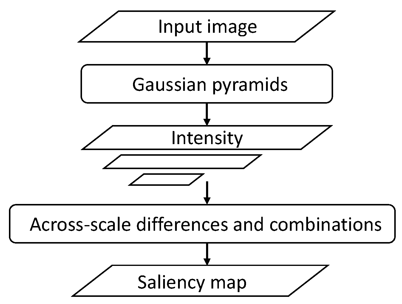
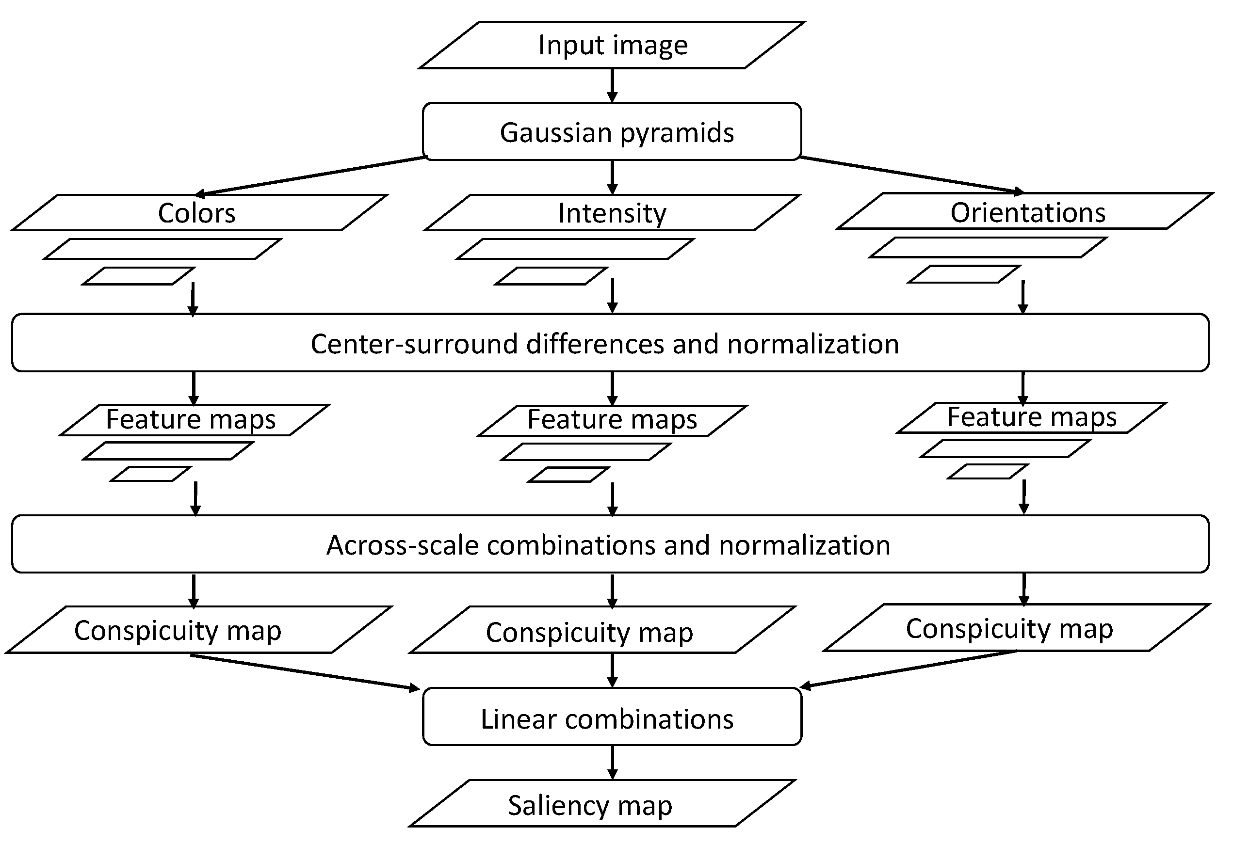
Itti’s model [40]: This model is among the early investigations on saliency computation. It is based on the “feature integration theory”, explaining human visual search strategies [51]. The flowchart of this model is presented in Figure 3. First, different low-level features, e.g., colors, intensities and orientations, are extracted independently of several spatial scales. Then, the center-surround differences, normalization and across-scale combination are sequentially operated on each feature to generate a conspicuity map, and the final saliency map is the sum of the three normalized conspicuity maps on the hypothesis that different features contribute independently to the saliency map.
-
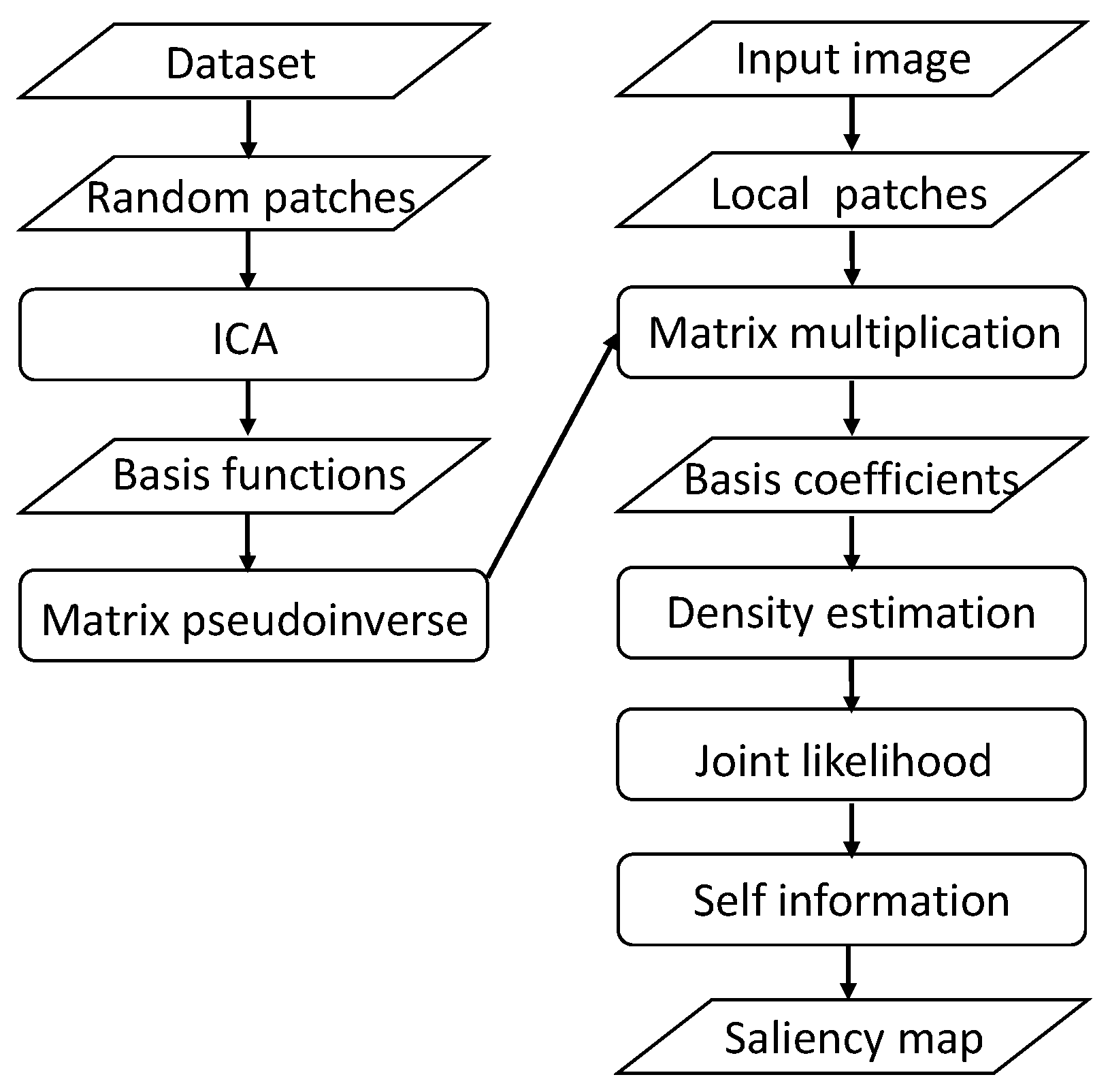
Attention by information maximization (AIM) [41]: This model is rooted in information theory, where the saliency is determined by quantifying Shannon’s self-information of each local image patch. It consists of two stages: independent feature extraction and estimation of Shannon’s measure of self-information. In the first step, to analyze features independently, the independent coefficients corresponding to the contribution of different features are computed using independent component analysis (ICA). In the second step, the distribution of each basis coefficient across the entire image is estimated, and Shannon’s measure of self-information is finally computed from the joint distribution. The flowchart of this model is shown in Figure 4.
-
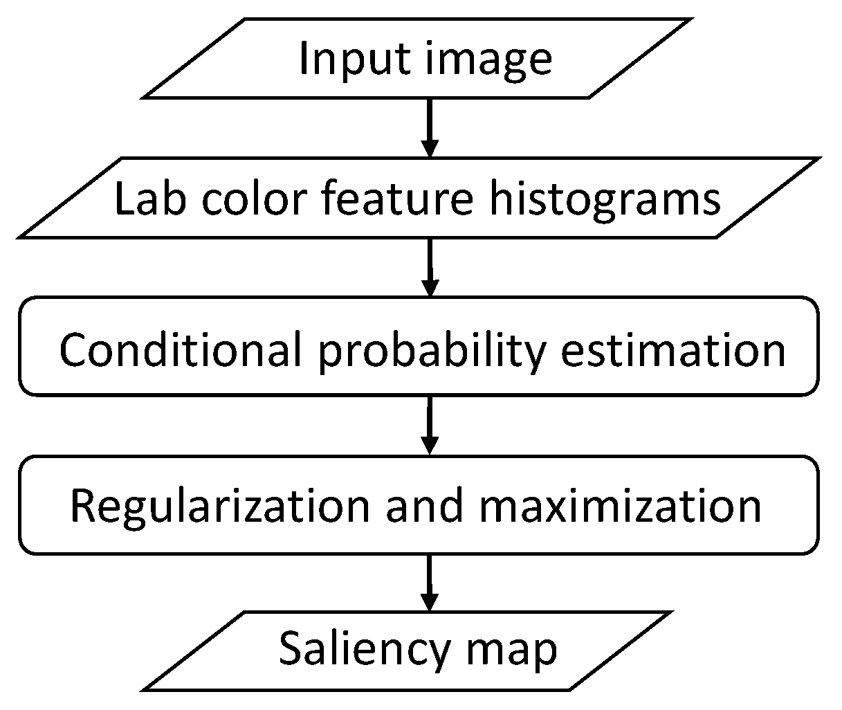
Salient segmentation (SEG) [42]: This uses a statistical framework and local feature contrast to define the saliency measure. Considering a rectangular window W composed of two disjoint parts, an inner window I and the border B, one can assume that the points in I are salient, while B belongs to the background. Define a random variable Z describing the distribution of pixels in W; the saliency measure of a point x I is thus defined to be the conditional probability,
S S E G ( x ) = p Z ( Z I | F ( Z ) Q F ( x ) )
where F denotes the Lab color feature map, which maps every point x to a certain feature F ( x ) , and Q F ( x ) denotes the bin that contains F ( x ) . After computing the saliency value of each pixel in a sliding window across the image, regularization and maximization are performed to produce a more robust saliency map. The flowchart of this model is shown in Figure 5.
-
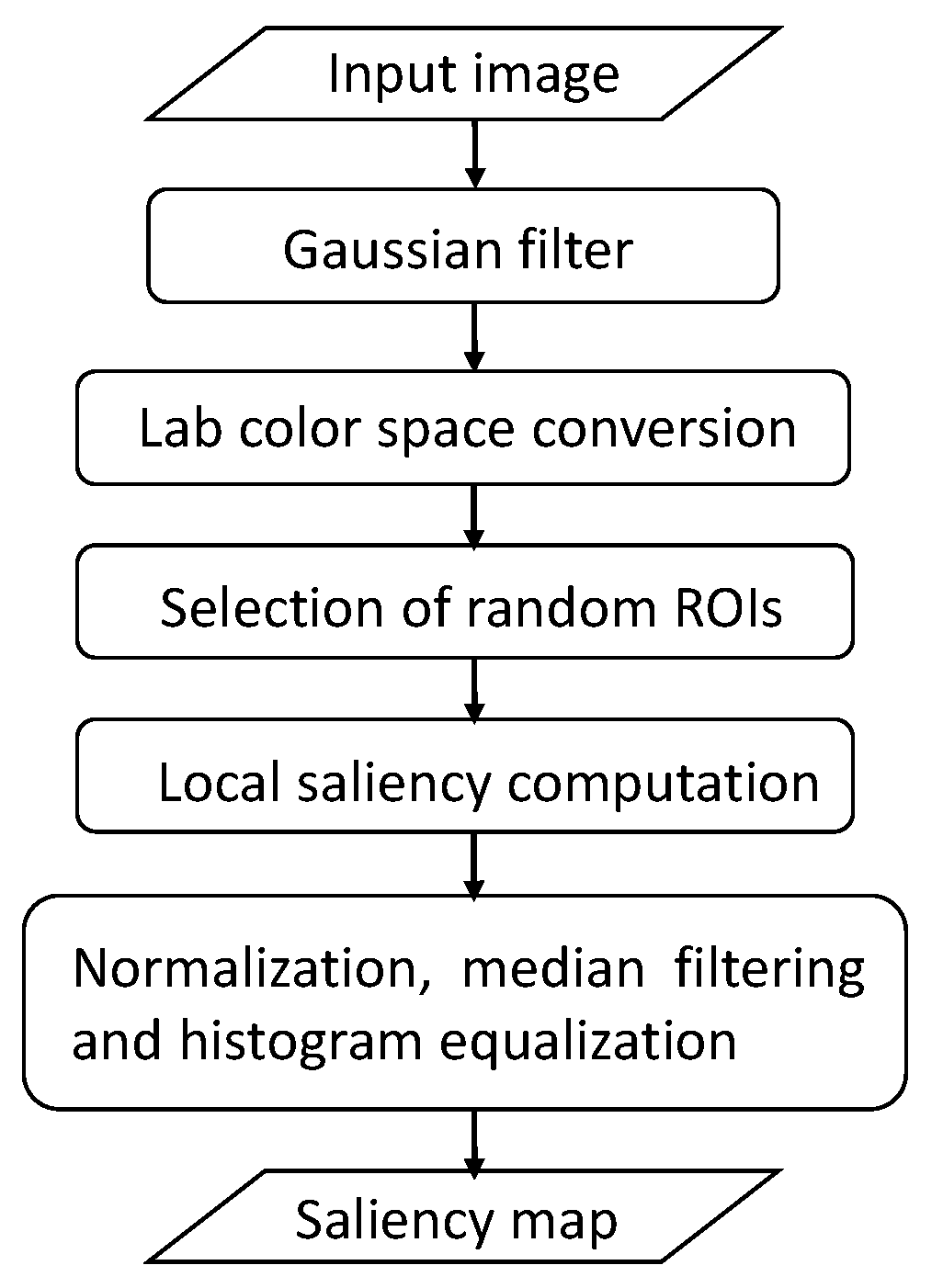
Random center-surround (RCS) saliency [43]: This model is based on computing local saliency over random rectangular regions of interest; see Figure 6. Given an image f : Ω R D with D channels, for each channel, n sub-windows are randomly generated with a uniform distribution. In the d-th channel, the local saliency of a point x is defined as the sum of the absolute differences between the pixel intensity and the mean intensity of the random sub-windows in which it is contained. The global saliency map is then computed by fusing the channel-specific saliency maps by a pixel-wise Euclidean norm. Furthermore, normalization, median filtering and histogram equalization are applied to the global saliency map to preserve edges, eliminate noise and enhance the contrast.
Figure 2. Flowchart of the SIFT detector.
Remotesensing 07 14988 g002
Figure 3. Flowchart of Itti’s saliency model.
Remotesensing 07 14988 g003
Figure 4. Flowchart of the attention by information maximization (AIM) saliency model.
Remotesensing 07 14988 g004
Figure 5. Flowchart of the SEG saliency model.
Remotesensing 07 14988 g005
The response maps of different sampling methods on two example images of the UC-Merced dataset are presented in Figure 7. For saliency-based sampling, the saliency maps are linearly normalized to be in the range of [ 0 , 255 ] as the response maps. The response map of random sampling is produced from an independent uniform distribution between [ 0 , 255 ] . These maps are of the same size as the treated images, and they are used as masks to guide the sampling procedure: the brighter the region, the more likely it is to be sampled from the image.
Figure 6. Flowchart of the RCS saliency model.
Remotesensing 07 14988 g006
Figure 7. The response maps of different sampling methods on two example images from the UC-Merced dataset. For saliency-based sampling, the saliency maps are linearly normalized to be in the range of [ 0 , 255 ] as the response maps. The response map of random sampling is produced from an independent uniform distribution between [ 0 , 255 ] . These maps are of the same size as the treated images, and they can be used as masks to guide the sampling procedure: the brighter the region, the more likely it is to be sampled from the image.
Remotesensing 07 14988 g007

3.3. Evaluating the Sampling Performances

To quantitatively evaluate the performances of different sampling strategies, we measure them using the classification overall accuracy (OA). It is defined as the number of correctly-predicted images divided by the total number of test images. In our experiments, we do not compute the Kappa coefficient for each method, because the datasets that we use are uniformly distributed among the classes, and thus, the Kappa coefficient is proportional to OA.
For fair comparisons, we fix the sampling ratio of different sampling methods to select the same number of patches. At each sampling ratio from 0 . 01 to one, we compute the OA corresponding to each sampling method. Thus, we can obtain an OA curve with respect to r for each sampling method.

4. Testing Datasets

In order to evaluate different sampling strategies in the scene classification of high-spatial resolution remote sensing imagery, we look for public datasets of original and optical high-spatial resolution remote sensing imagery. However, observe that the number of such available datasets is very limited, except the UC-Merced dataset [1]. It is worth noticing that, unlike pixel-level land cover/use classification, where the spectral information of pixels plays a key role, scene classification pay more attention to the spatial pattern (relative spatial configuration) of pixels, and the true spectral value of pixel is less important. Moreover, it has been reported that even on the task of pixel-level land use/cover classification, Google Earth imagery, an important source of free aerial images in high-spatial resolution, which offers RGB renderings of the original high-resolution remote sensing imagery, can perform comparably with original HSR-RS imagery: QuickBird imagery [52]. Thus, it is feasible to use high-resolution Google Earth imagery to evaluate different scene classification procedures.
In our experiments, we used one public dataset of original high-spatial resolution remote sensing imagery, i.e., the UC-Merced dataset [1], and one public dataset collected from Google Earth imagery, i.e., RS19 dataset [53], for evaluating, and each of them will be described in what follows.

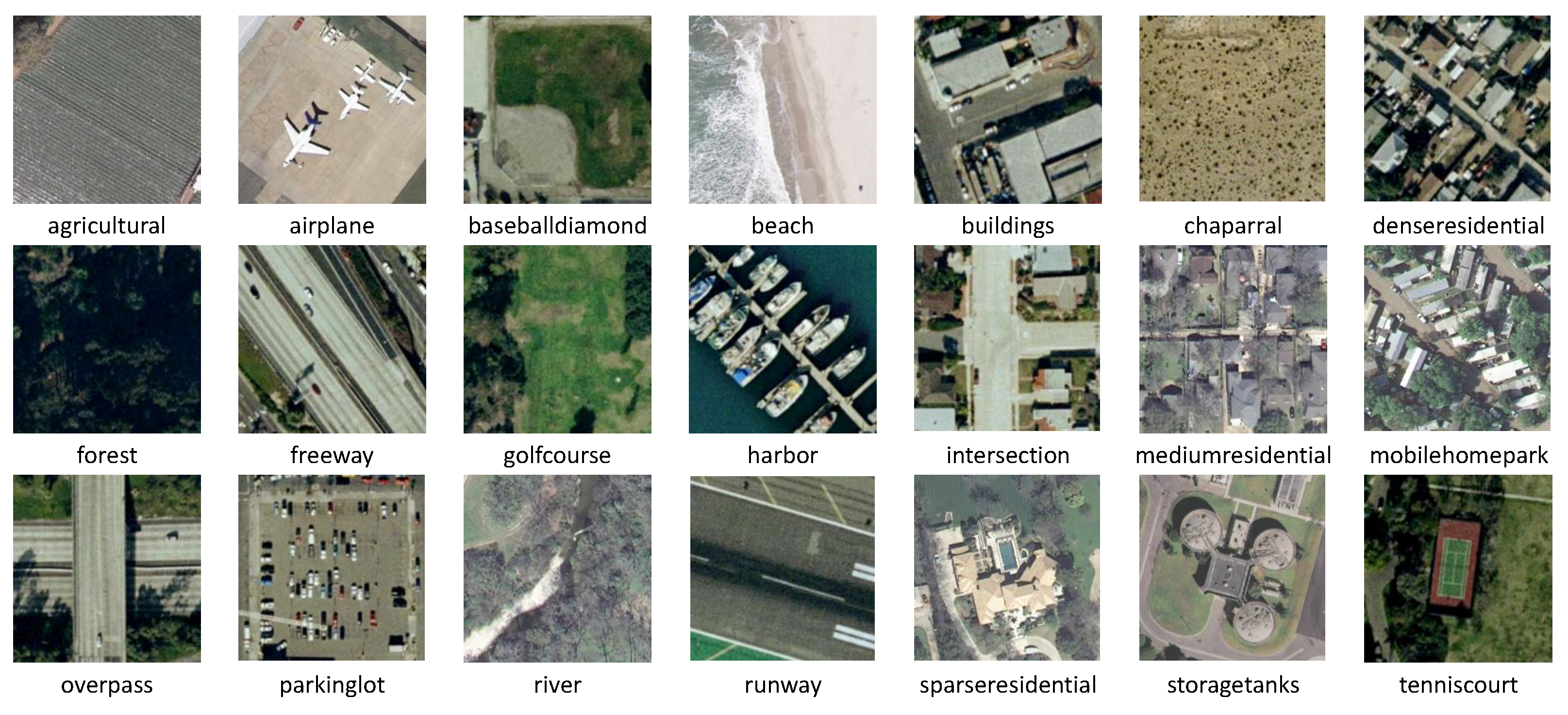
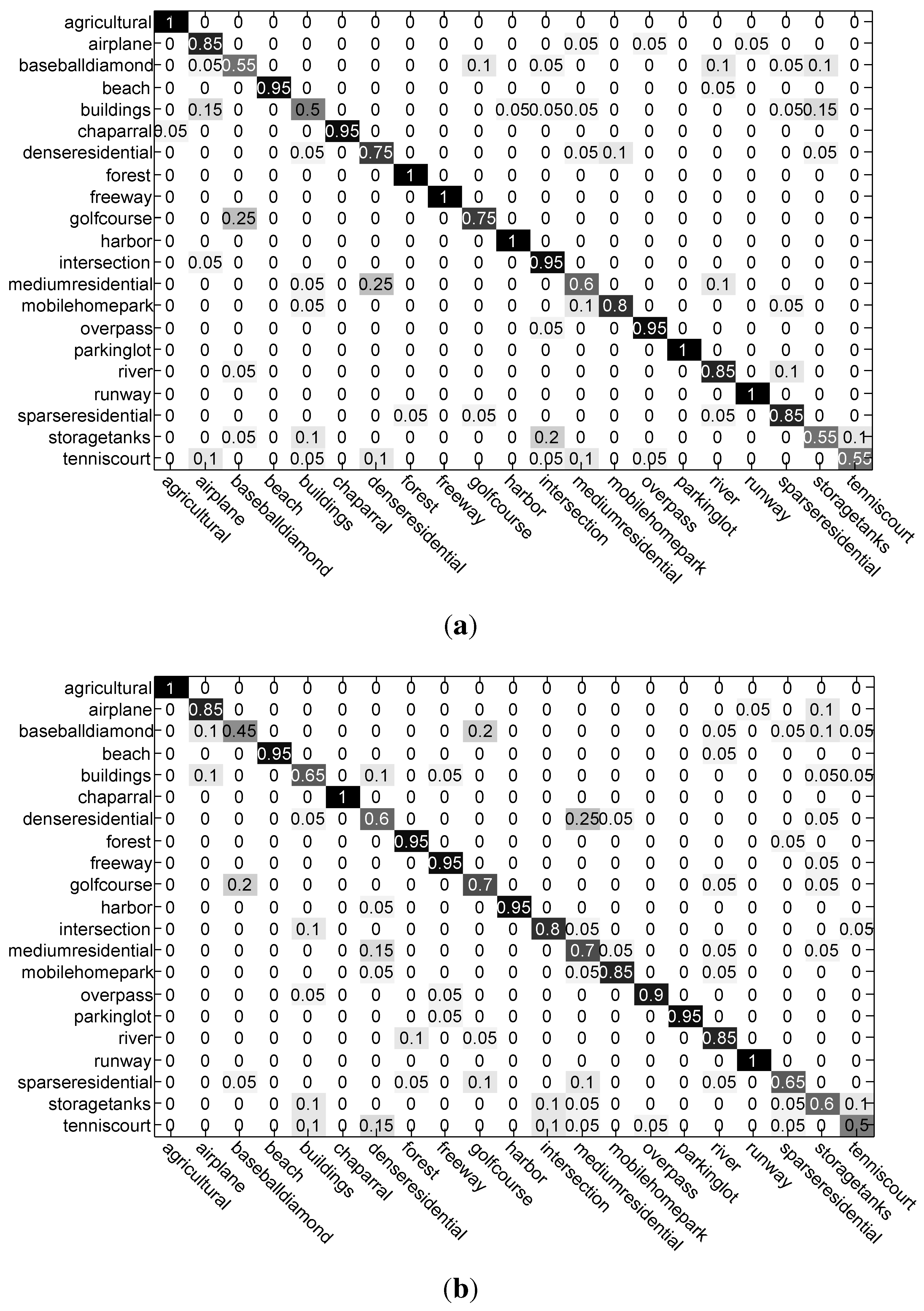
4.1. UC-Merced Dataset
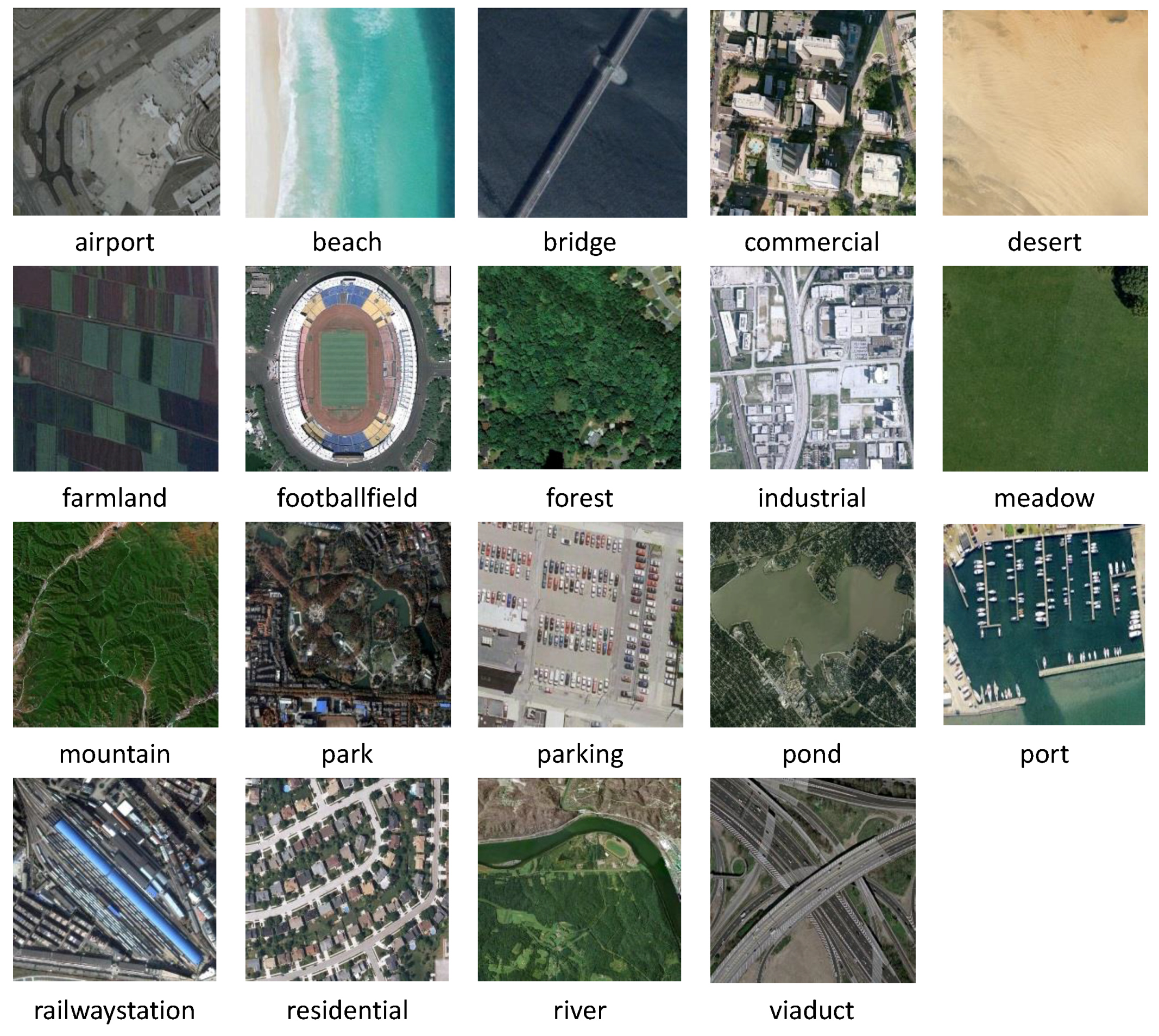
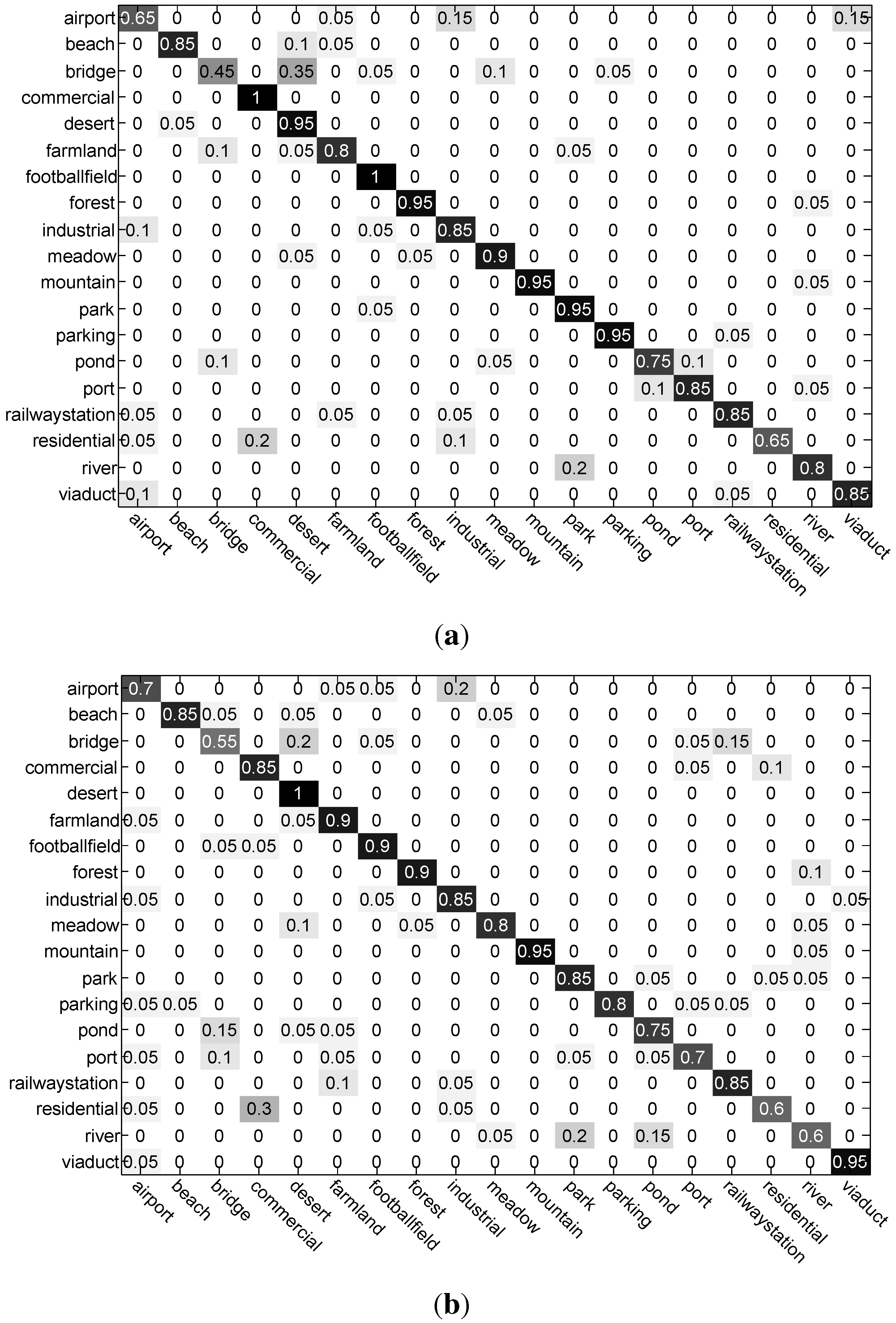
The UC-Merced dataset [1] contains 21 scene categories, with 100 samples per class. Figure 8 presents a few example images representing different scenes that are included in this dataset. The images are selected from optical aerial orthoimagery with a pixel resolution of one foot. The original large images were downloaded from the United States Geological Survey (USGS) National Map of the following U.S. regions: Birmingham, Boston, Buffalo, Columbus, Dallas, Harrisburg, Houston, Jacksonville, Las Vegas, Los Angeles, Miami, Napa, New York, Reno, San Diego, Santa Barbara, Seattle, Tampa, Tucson and Ventura. They are cropped into 256 by 256 pixels, among which there are a total of 2100 images manually selected and uniformly labeled into the following 21 classes: agricultural, airplane, baseball diamond, beach, buildings, chaparral, dense residential, forest, freeway, golf course, harbor, intersection, medium density residential, mobile home park, overpass, parking lot, river, runway, sparse residential, storage tanks and tennis courts. This dataset is widely used and has been reported to be challenging, because it contains highly overlapping classes (e.g., dense residential, medium residential and sparse residential), which mainly differ in the density of structures and are difficult to distinguish even for humans.
Figure 8. UC-Merced dataset: some example images are displayed. It contains 21 scene categories, with 100 samples per class. The images are of a size of 256 × 256 pixels with a pixel resolution of one foot.
Remotesensing 07 14988 g008
Figure 9. RS19dataset: this contains 19 classes of scenes in optical high-spatial resolution satellite imagery that are exported from Google Earth with various resolutions. For each class, there are 50 samples, and the image sizes are 600 × 600 pixels.
Remotesensing 07 14988 g009

4.2. RS19 Dataset

The RS19 dataset [53] contains 19 classes of scenes in optical high-spatial resolution satellite imagery that are exported from Google Earth, the images of which have a fixed size of 600 by 600 pixels with various pixel resolutions of up to half a meter. Figure 9 presents some example images of each class. The 19 classes of meaningful scenes include airport, beach, bridge, river, forest, meadow, pond, parking, port, viaduct, residential area, industrial area, commercial area, desert, farmland, football field, mountain, park and railway station. For each class, there are 50 samples. Thus, the dataset is composed of a 19-class satellite scene with a total number of 950 images. Note that the image samples of the same class are collected from different regions all around the world; thus, it is very challenging due to the changes in resolution, scale, orientation and illuminations of the images.

5. Experimental Results and Analysis

In this section, we describe the comparative results of different sampling strategies on the two testing datasets for scene classification in optical HSR-RS images.

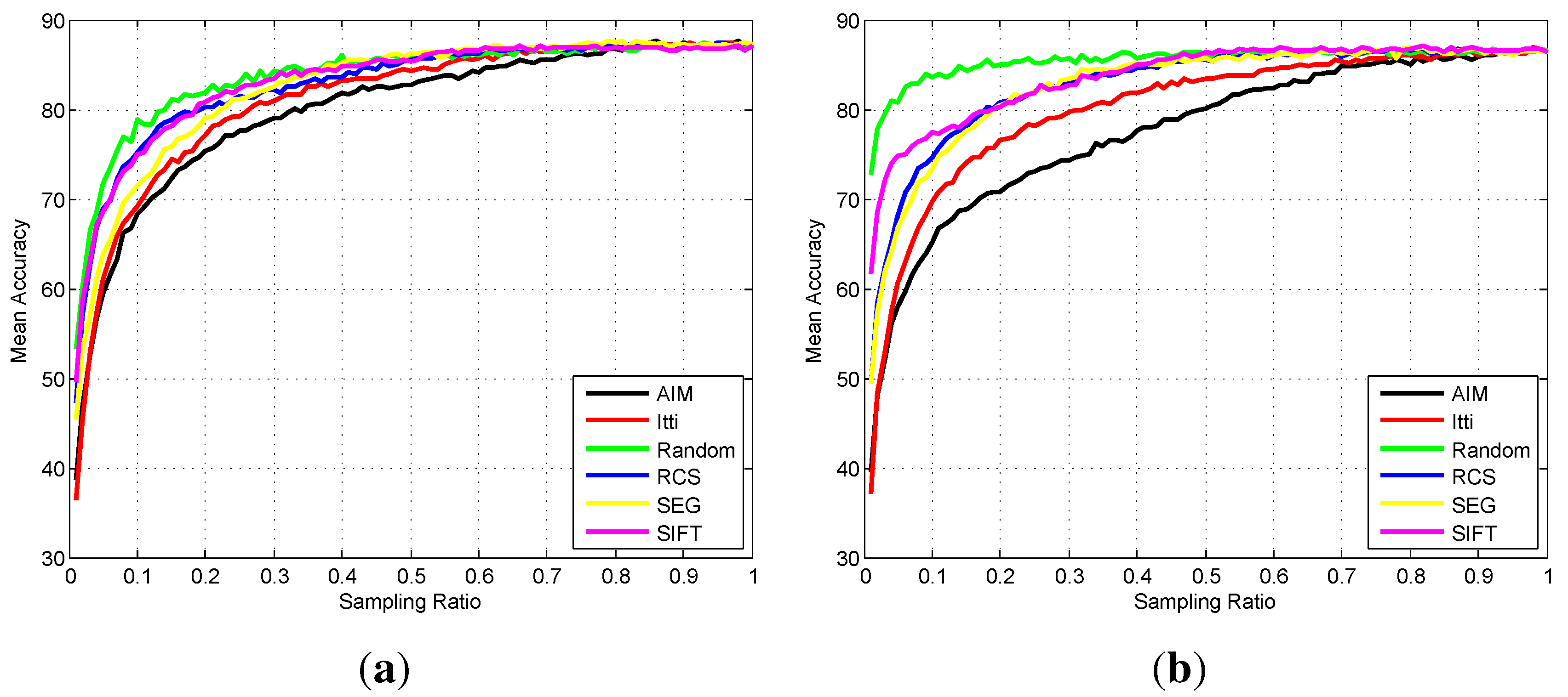
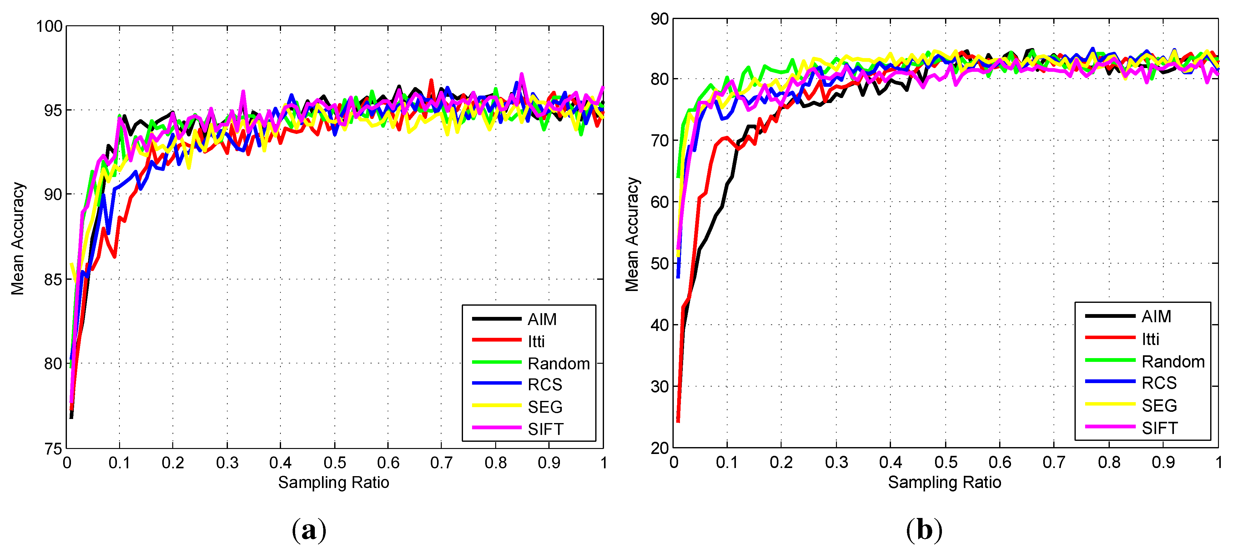
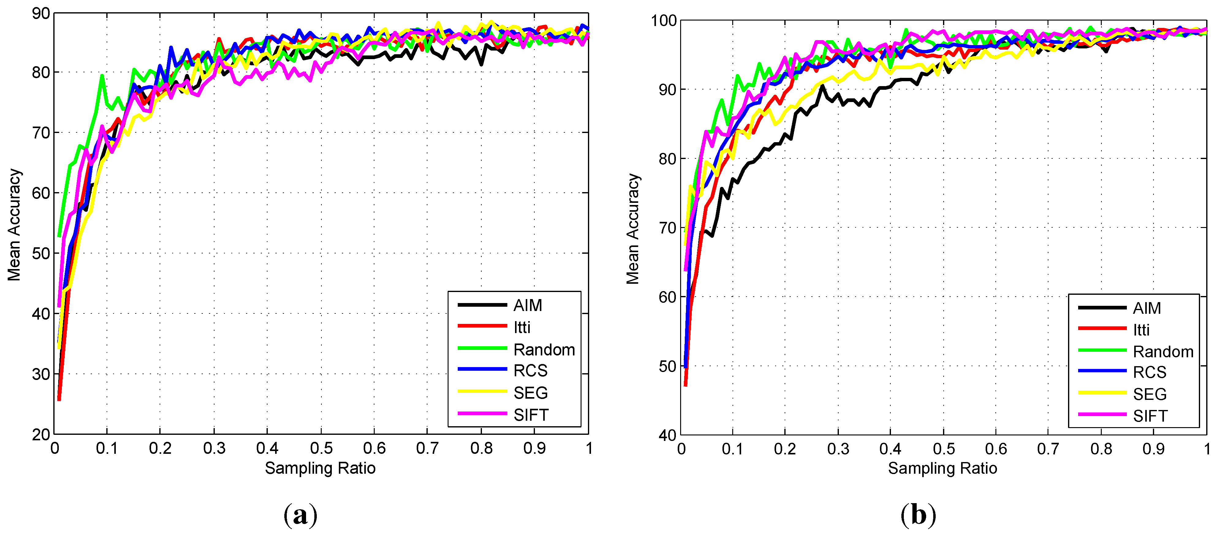
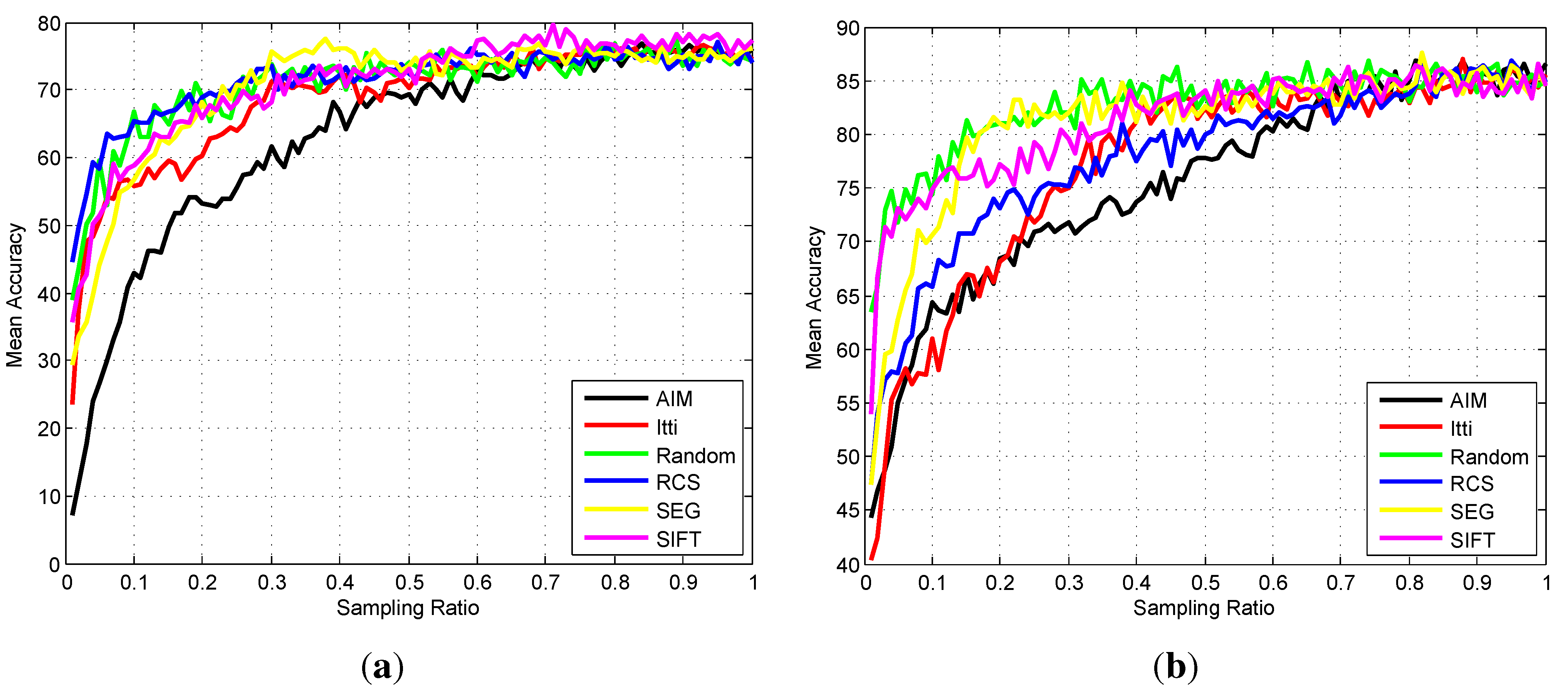
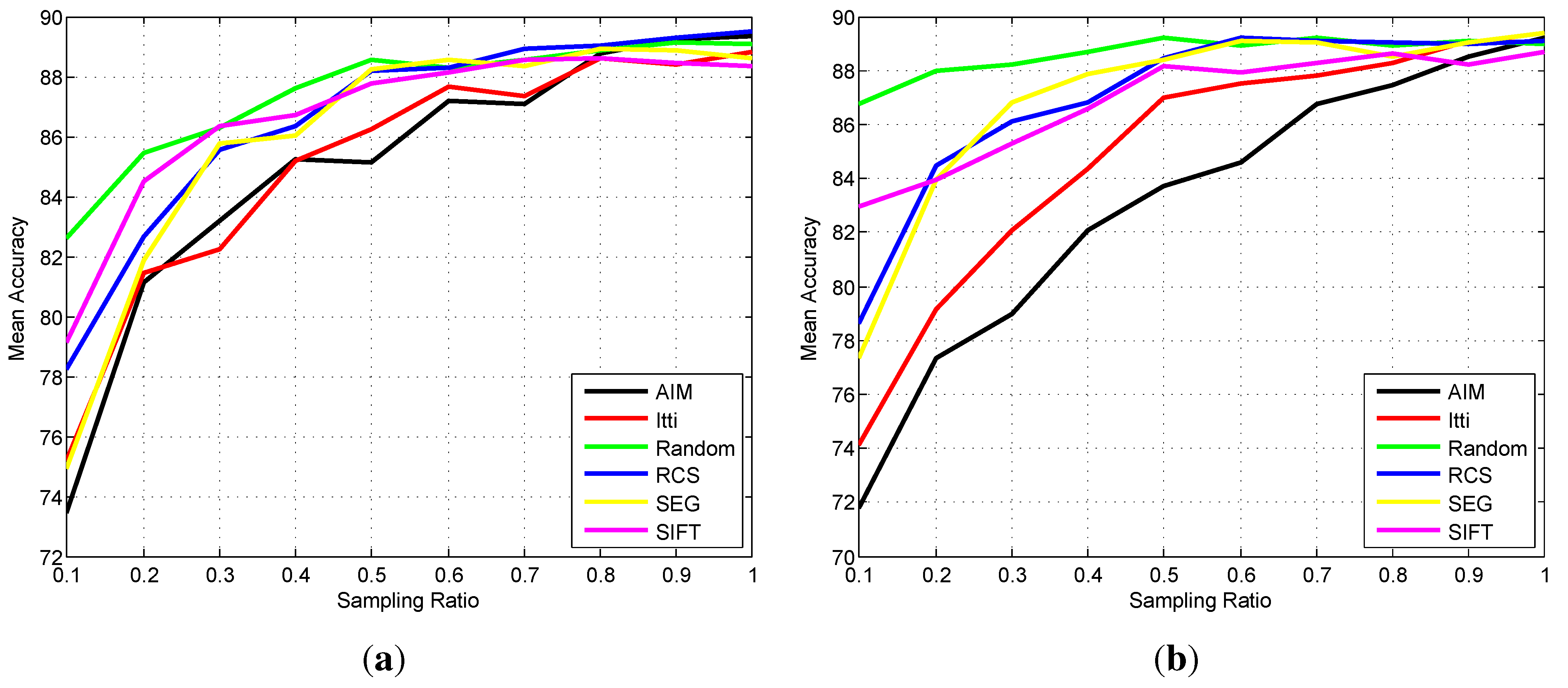
5.1. Overall Testing

Figure 10 shows the overall classification accuracy using different sampling methods on the UC-Merced dataset and the RS19 dataset. The horizontal axis indicates the sampling ratio r, and the vertical axis represents the average of OA for 100 repetitions corresponding to different sampling ratios. At the same sampling ratio, there are the same number of patches to be selected to form the representative set for every image using different sampling methods. Here, we just demonstrate the average of OA for legibility; all of their standard deviations are within 2 % , which is reasonable.
Figure 10. Comparisons of the overall classification accuracy using different sampling methods on the UC-Merced dataset (a) and the RS19 dataset (b).
Remotesensing 07 14988 g010
As shown in Figure 10a, all of the curves share the same properties: they are generally increasing, but with slight shakes that are caused by the random selection of the training set in the SVM classifier; these are within the standard deviation and are thus reasonable. We can also learn from the results that as the sampling ratio becomes larger, the increase of the curves become smaller, and some of the curves almost become flat when the sampling ratio is larger than 0 . 7 . This result implies that the different sampling methods will provide similar results when the information contained in the sampled patches approaches a certain degree. However, random sampling obviously outperforms the other approaches when the sampling ratio is low. Comparing the sampling strategies on the RS19 dataset in Figure 10b, we can obtain the same conclusion with the UC-Merced dataset that random sampling has an evident advantage over the other sampling methods at low sampling ratios.
From the overall accuracy of the two datasets, we can come to the following conclusions:
-
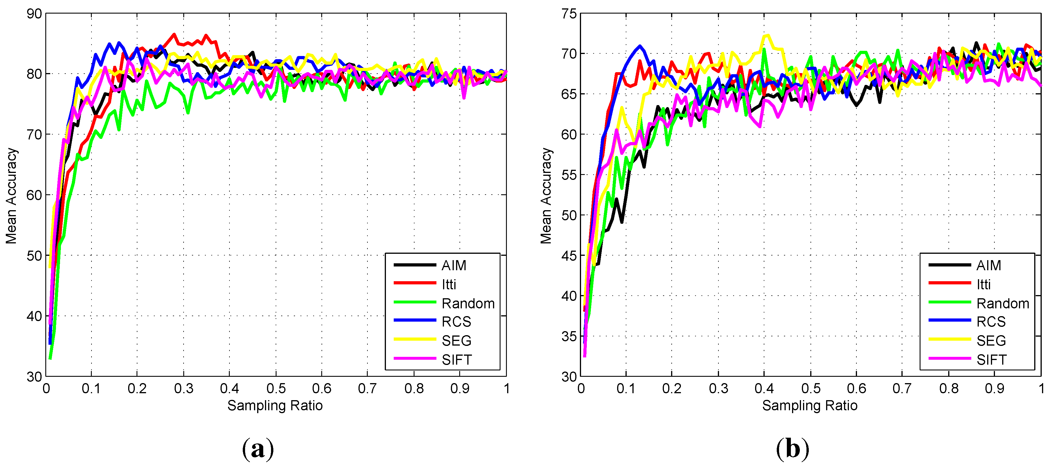
Random sampling is obviously better than the other sampling methods, such as various saliency-based sampling methods, when the sampling ratio is low, primarily because it can extract balanced land cover information, which can help to improve the performance in scene classification.
-
As the sampling ratio become larger, the differences among the sampling methods become smaller because the information extracted becomes richer. Thus, all of the sampling methods provide comparable results.
-
In general, random sampling can provide comparable and even better performance regardless of the sampling ratio.
Figure 11. Comparisons of the confusion matrices using random sampling (a) and the SIFT sampling (b) method on the UC-Merced dataset when the sampling ratio is equal to 0 . 2 .
Remotesensing 07 14988 g011
Note that random sampling outperforms other approaches, particularly at low sampling ratios; we further analyze the corresponding confusion matrices. Figure 11 shows the confusion matrices using random sampling and the SIFT sampling method on the UC-Merced dataset with the fixed training set at a low sampling ratio (e.g., 0 . 2 ). The reason why we choose to draw the confusion matrix of the SIFT sampling method is that it has the best result among saliency-based ones at this point. By further comparing these two confusion matrices, we can see that random sampling has far better performances on baseball diamond, dense residential, intersection and sparse residential, whereas SIFT performs better on buildings and storage tanks. A similar phenomenon also appears on the RS19 dataset (see Figure 12) by comparing random sampling with the best saliency-based sampling, RCS when r = 0 . 2 . For commercial, meadow, park, parking and river, random sampling performs far better than RCS, whereas for airport, bridge and viaduct, the opposite is true. Intuitively, some sampling methods may be helpful for some special types of scenes. Thus, we roughly divide the scene in optical HSR-RS images into four types, namely single texture scenes, multiple texture scenes, object-based scenes and structural scenes, and we analyze the classification performance on each type of scene in the following.
Figure 12. Comparisons of the confusion matrices using random sampling (a) and the RCS sampling (b) method on the RS19 dataset when the sampling ratio is equal to 0 . 2 .
Remotesensing 07 14988 g012

5.2. Testing on Single Texture Scenes

Figure 13 shows two examples of the single texture scenes, which mainly contain only one kind of textures, like agricultural, meadow, chaparral, forest, mountain, etc. From the curves of agricultural, we can see that most of the sampling methods become flat when the sampling ratio becomes larger than 0 . 4 , and this is similar for the meadow. This could be explained by the fact that this type of scene mainly consists of a single texture with large information redundancy and, thus, can be easily distinguished using a small part of the land cover features. For single texture scenes, the performances of most sampling methods are similar and can become stable at low sampling ratios, e.g., 0.4.
However, when the sample images contain some disturbing objects, like a footpath in the agricultural, some saliency-based methods will firstly extract the patches that belong to it; thus, this will result in low classification accuracy at low sampling ratios, and this can be observed from the curves of Itti in Figure 13. Therefore, for the single texture scenes with high information redundancy, we better use random sampling at a very low sampling ratio to select the patches, since it can obtain similar or even higher classification accuracy compared to the saliency-based ones.
Figure 13. Comparisons of the classification accuracy using different sampling methods on the scenes of agricultural (a) and meadow (b).
Remotesensing 07 14988 g013

5.3. Testing on Multiple Texture Scenes

This type of scene is composed of several textures, such as beach, river, etc. As this type needs to be classified by different texture features, like water, grass, trees and sands, most of the curves become stable after 60 % of patches are extracted and share a similar trend (see Figure 14). For saliency-based methods, they may firstly extract only one type of texture; therefore, random sampling performs better when the sampling ratio is low.
Figure 14. Comparisons of the classification accuracy using different sampling methods on river (a) and beach (b).
Remotesensing 07 14988 g014

5.4. Testing on Object-Based Scenes

Object-based scenes mainly consist of a clear object and its backgrounds, such as airplane and storage tanks. The result is very interesting (see Figure 15): that most curves drop slightly after increasing rapidly at the beginning and then become stable in the end. This phenomenon is due to the fact that the classification of this type of scene is similar to the object recognition problem in essence. Thus, most saliency-based methods can firstly extract the features of the objects, which can help to improve the performance. However, as the sampling ratio becomes higher, the features of the objects become less dominant for more background parts being extracted. Thus, the trend of the curves can be explained. Therefore, for this type of scene, saliency-based sampling with a low sampling ratio is preferred.
Figure 15. Comparisons of the classification accuracy using different sampling methods on airplane (a) and storage tanks (b).
Remotesensing 07 14988 g015

5.5. Testing on Structural Scenes

The last is composed of more complex scenes that contain densely-distributed structures and textures, such as buildings, commercial, and residential areas, among others. As shown in Figure 16, the curves of this type are completely increasing, which implies that the more information that is extracted, the better is the performance. This is because this type of scene classification not only depends on the different land cover features contained, but also on their different proportion. Therefore, random sampling with a high sampling ratio is the best for these types of complex scenes.
Note that when comparing the performances of each type of scene, the results may be inconsistent with the confusion matrices. For instance, in Figure 11, the accuracy of buildings using SIFT is better, whereas in Figure 16a, random sampling achieves a slightly higher accuracy than SIFT when r = 0 . 2 . This is caused by the selection of the training set: we fix the training set when computing the confusion matrices, whereas we randomly initialize the training set with 100 repetitions and compute the average when drawing the curves. Because there are only 20 images in each class for testing, the selection of the training set will have an important influence on the classification accuracy. Therefore, the confusion matrices are simply references for the analysis, and the curves provide more reliable results.
Figure 16. The classification accuracy using different sampling methods on buildings (a) and residential (b).
Remotesensing 07 14988 g016

5.6. Validation Experiment Using the Fisher Kernel Approach

The validation experiment results obtained using the Fisher kernel approach on the two datasets using different sampling methods are presented in Figure 17. From the experiment results presented in Figure 17, we can come to the same conclusions as with the BoVW model that random sampling has better performance than saliency-based ones at low sampling ratios and is comparative at high sampling ratios. Moreover, because saliency-based sampling methods need to spend a considerable amount of time on producing saliency maps of every image, random sampling has obvious advantages over saliency-based ones, not only in the overall classification accuracy, but also in the computing efficiency.
Figure 17. The classification accuracy using different sampling methods on the UC-Merced dataset (a) and the RS19 dataset (b) using the Fisher kernel framework.
Remotesensing 07 14988 g017

5.7. Discussion

From the above experimental results obtained using different feature learning frameworks, we can now reach the conclusion that random sampling has comparative and even better performance than other sampling methods overall. Although some saliency-based sampling methods may perform better on a certain type of scene (e.g., the object-based scenes), they cannot compete with random sampling on the entire dataset, particularly at low sampling ratios. In natural image classification [19], it has been concluded that random sampling only provides equal or better classification performance than the sophisticated multi-scale interest operators with a large number of patches, which is inconsistent with our results. This further proves our opinion that the conclusions from natural images cannot be directly transferred to optical HSR-RS imagery.
By further comparing the running time for producing response maps for a sample image using different sampling strategies on the two testing datasets in Table 2, we can see that random sampling has considerably higher computing efficiency than other approaches. Moreover, the saliency-based methods need to compute the saliency map for each sample image and save them for reuse in different sampling ratios, whereas for random sampling, we can use a single response map to sample all of the images. Therefore, random sampling has substantially lower space and time complexity.
Table 2. Running time for producing response maps for a sample image using different sampling strategies on two testing datasets.
Sampling StrategyRandomSIFTIttiAIMSEGRCS
UC-Merced dataset ( 256 × 256 pixels)0.002 s0.02 s0.2 s4 s8.2 s0.5 s
RS19 dataset ( 600 × 600 pixels)0.01 s0.02 s0.4 s28 s25 s2.3 s
Overall, because scene classification datasets are obviously composed of various types of scenes, both simple textural scenes and complex structural scenes, random sampling is the first choice because of its robustness, good performance and lower space and time complexity.

6. Conclusions

This paper investigates the performance of various sampling strategies in the scene classification of optical high-spatial resolution remote sensing imagery. To compare different sampling strategies, we adopt the classic bag-of-visual-words model to construct a unified scheme embedded with different sampling methods, e.g., random sampling and various saliency-based sampling methods. We conduct experiments on two commonly-used datasets in the literature: the UC-Merced dataset and the RS19 dataset. Based on the experimental results, we reach the following consistent and meaningful conclusions: although saliency-based methods may show a slight improvement in some specific types of scene classification, they cannot compete with random sampling on the entire dataset. Therefore, random sampling is the best choice for improving the classification performance in the scene classification of optical high-spatial resolution remote sensing imagery. Moreover, random sampling possesses low time and space complexities compared to saliency-based approaches. Furthermore, the results presented in this paper can be applied to many scene classification approaches for optical HSR-RS images, because the results of our validation experiment using the Fisher kernel framework provide the same conclusions as those obtained with the bag-of-visual-words model.

Acknowledgments

The authors would like to thank all of the researchers who kindly shared the codes used in our studies. This research was supported by the National Natural Science Foundation of China under Contract No. 91338113 and No. 41501462, and it was partially funded by the Wuhan Municipal Science and Technology Bureau, with Chen-Guang Grant 2015070404010182.

Author Contributions

Jingwen Hu and Gui-Song Xia had the original idea for the study. Gui-Song Xia supervised the research and contributed to the article’s organization. Fan Hu contributed to part of the experiments. Liangpei Zhang contributed to the discussion of the design. Jingwen Hu drafted the manuscript, which was revised by all of the authors. All of the authors read and approved the submitted manuscript.

Conflicts of Interest

The authors declare no conflict of interest.

References

  1. Yang, Y.; Newsam, S. Bag-of-visual-words and spatial extensions for land-use classification. In Proceedings of the 18th SIGSPATIAL International Conference on Advances in Geographic Information Systems, San Jose, CA, USA, 2–5 November 2010; pp. 270–279.
  2. Sheng, G.; Yang, W.; Xu, T.; Sun, H. High-resolution satellite scene classification using a sparse coding based multiple feature combination. Int. J. Remote Sens. 2012, 33, 2395–2412. [Google Scholar] [CrossRef]
  3. Zhao, B.; Zhong, Y.; Zhang, L. Hybrid generative/discriminative scene classification strategy based on latent dirichlet allocation for high spatial resolution remote sensing imagery. In Proceedings of the IEEE International Geoscience and Remote Sensing Symposium (IGARSS), Melbourne, VIC, Australia, 21–26 July 2013; pp. 196–199.
  4. Shao, W.; Yang, W.; Xia, G.S. Extreme value theory-based calibration for the fusion of multiple features in high-resolution satellite scene classification. Int. J. Remote Sens. 2013, 34, 8588–8602. [Google Scholar] [CrossRef]
  5. Hu, F.; Yang, W.; Chen, J.; Sun, H. Tile-level annotation of satellite images using multi-level max-margin discriminative random field. Remote Sens. 2013, 5, 2275–2291. [Google Scholar] [CrossRef]
  6. Shao, W.; Yang, W.; Xia, G.S.; Liu, G. A hierarchical scheme of multiple feature fusion for high-resolution satellite scene categorization. In Computer Vision Systems; Springer: Berlin, Germany, 2013; pp. 324–333. [Google Scholar]
  7. Sridharan, H.; Cheriyadat, A. Bag of Lines (BoL) for Improved Aerial Scene Representation. IEEE Trans. Geosci. Remote Sens. Lett. 2014, 12, 676–680. [Google Scholar] [CrossRef]
  8. Kusumaningrum, R.; Wei, H.; Manurung, R.; Murni, A. Integrated visual vocabulary in latent Dirichlet allocation-based scene classification for IKONOS image. J. Appl. Remote Sens. 2014. [Google Scholar] [CrossRef]
  9. Zhao, L.; Tang, P.; Huo, L. A 2-D wavelet decomposition-based bag-of-visual-words model for land-use scene classification. Int. J. Remote Sens. 2014, 35, 2296–2310. [Google Scholar]
  10. Cheriyadat, A.M. Unsupervised feature learning for aerial scene classification. IEEE Trans. Geosci. Remote Sens. 2014, 52, 439–451. [Google Scholar] [CrossRef]
  11. Dos Santos, J.; Penatti, O.; Gosselin, P.H.; Falcao, A.X.; Philipp-Foliguet, S.; Torres, D.S. Efficient and effective hierarchical feature propagation. IEEE J. Sel. Top. Appl. Earth Obs. Remote Sens. 2014, 7, 4632–4643. [Google Scholar] [CrossRef]
  12. Chen, S.; Tian, Y. Pyramid of Spatial Relatons for Scene-Level Land Use Classification. IEEE Trans. Geosci. Remote Sens. 2015, 53, 1947–1957. [Google Scholar] [CrossRef]
  13. Zhang, F.; Du, B.; Zhang, L. Saliency-Guided Unsupervised Feature Learning for Scene Classification. IEEE Trans. Geosci. Remote Sens. 2015, 53, 2175–2184. [Google Scholar] [CrossRef]
  14. Hu, F.; Xia, G.S.; Wang, Z.; Huang, X.; Zhang, L.; Sun, H. Unsupervised Feature Learning Via Spectral Clustering of Multidimensional Patches for Remotely Sensed Scene Classification. IEEE J. Sel. Top. Appl. Earth Obs. Remote Sens. 2015, 8, 2015–2030. [Google Scholar] [CrossRef]
  15. Penatti, O.A.B.; Nogueira, K.; dos Santos, J.A. Do Deep Features Generalize From Everyday Objects to Remote Sensing and Aerial Scenes Domains? In Proceedings of the IEEE Conference on Computer Vision and Pattern Recognition, Boston, MA, USA, 8–10 June 2015.
  16. Yang, W.; Yin, X.; Xia, G.S. Learning High-level Features for Satellite Image Classification with Limited Labeled Samples. IEEE Trans. Geosci. Remote Sens. 2015, 53, 4472–4482. [Google Scholar] [CrossRef]
  17. Hu, F.; Wang, Z.; Xia, G.S.; Zhang, L. Fast binary coding for satellite image scene classification. In Proceedings of the IEEE International Geoscience and Remote Sensing Symposium (IGARSS), Mailan, Italy, 26–31 July 2015.
  18. Fei-Fei, L.; Perona, P. A bayesian hierarchical model for learning natural scene categories. In Proceedings of the IEEE Conference on Computer Vision and Pattern Recognition, San Diego, CA, USA, 20–25 June 2005; Volume 2, pp. 524–531.
  19. Nowak, E.; Jurie, F.; Triggs, B. Sampling strategies for bag-of-features image classification. In Proceedings of the European Conference on Computer Vision, Graz, Austria, 7–13 May 2006; pp. 490–503.
  20. Payne, A.; Singh, S. A benchmark for indoor/outdoor scene classification. In Pattern Recognition and Image Analysis; Springer: Berlin, Germany, 2005; pp. 711–718. [Google Scholar]
  21. Xiao, J.; Hays, J.; Ehinger, K.; Oliva, A.; Torralba, A. Sun database: Large-scale scene recognition from abbey to zoo. In Proceedings of the IEEE Conference on Computer Vision and Pattern Recognition, San Francisco, CA, USA, 13–18 June 2010; pp. 3485–3492.
  22. Perronnin, F.; Sánchez, J.; Mensink, T. Improving the Fisher Kernel for Large-scale Image Classification. In Proceedings of the European Conference on Computer Vision, Heraklion, Crete, Greece, 5–11 September 2010; pp. 143–156.
  23. Lazebnik, S.; Schmid, C.; Ponce, J. Beyond bags of features: Spatial pyramid matching for recognizing natural scene categories. In Proceedings of the IEEE Conference on Computer Vision and Pattern Recognition, New York, NY, USA, 17–22 June 2006; Volume 2, pp. 2169–2178.
  24. Bosch, A.; Zisserman, A.; Muñoz, X. Scene classification via pLSA. In Proceedings of the European Conference on Computer Vision, Graz, Austria, 7–13 May 2006; pp. 517–530.
  25. Bosch, A.; Zisserman, A.; Muñoz, X. Scene classification using a hybrid generative/discriminative approach. IEEE Trans. Pattern Anal. Mach. Intell. 2008, 30, 712–727. [Google Scholar] [CrossRef] [PubMed]
  26. Yang, J.; Yu, K.; Gong, Y.; Huang, T. Linear spatial pyramid matching using sparse coding for image classification. In Proceedings of the IEEE Conference on Computer Vision and Pattern Recognition, Miami, FL, USA, 20–25 June 2009; pp. 1794–1801.
  27. Mikolajczyk, K.; Schmid, C. Scale & affine invariant interest point detectors. Int. J. Comput. Vis. 2004, 60, 63–86. [Google Scholar] [CrossRef]
  28. Lowe, D.G. Distinctive image features from scale-invariant keypoints. Int. J. Comput. Vis. 2004, 60, 91–110. [Google Scholar] [CrossRef]
  29. Xia, G.S.; Delon, J.; Gousseau, Y. Accurate junction detection and characterization in natural images. Int. J. Comput. Vis. 2014, 106, 31–56. [Google Scholar] [CrossRef]
  30. Sivic, J.; Zisserman, A. Video Google: A text retrieval approach to object matching in videos. In Proceedings of the IEEE International Conference on Computer Vision, Nice, France, 13–16 October 2003; pp. 1470–1477.
  31. Lazebnik, S.; Schmid, C.; Ponce, J. A sparse texture representation using affine-invariant regions. In Proceedings of the IEEE Conference on Computer Vision and Pattern Recognition, Madison, WI, USA, 18–20 June 2003; Volume 2, pp. II-319–II-324.
  32. Csurka, G.; Dance, C.; Fan, L.; Willamowski, J.; Bray, C. Visual categorization with bags of keypoints. In Proceedings of the European Conference on Computer Vision, Prague, Czech Republic, 11–14 May 2004; Volume 1, pp. 1–2.
  33. Yang, J.; Jiang, Y.G.; Hauptmann, A.G.; Ngo, C.W. Evaluating bag-of-visual-words representations in scene classification. In Proceedings of 9th ACM SIGMM International Workshop on Multimedia Information Retrieval, Augsburg, Germany, 24–29 September 2007; pp. 197–206.
  34. Gokalp, D.; Aksoy, S. Scene classification using bag-of-regions representations. In Proceedings of the IEEE Conference on Computer Vision and Pattern Recognition, Minneapolis, MN, USA, 17–22 June 2007; pp. 1–8.
  35. Jurie, F.; Triggs, B. Creating efficient codebooks for visual recognition. In Proceedings of the IEEE International Conference on Computer Vision, Beijing, China, 17–21 October 2005; Volume 1, pp. 604–610.
  36. Winn, J.; Criminisi, A.; Minka, T. Object categorization by learned universal visual dictionary. In Proceedings of the IEEE International Conference on Computer Vision, Beijing, China, 17–21 October 2005; Volume 2, pp. 1800–1807.
  37. Siagian, C.; Itti, L. Rapid biologically-inspired scene classification using features shared with visual attention. IEEE Trans. Pattern Anal. Mach. Intell. 2007, 29, 300–312. [Google Scholar] [CrossRef] [PubMed]
  38. Borji, A.; Itti, L. Scene classification with a sparse set of salient regions. In Proceedings of the IEEE International Conference on Robotics and Automation, Shanghai, China, 9–13 May 2011; pp. 1902–1908.
  39. Sharma, G.; Jurie, F.; Schmid, C. Discriminative spatial saliency for image classification. In Proceedings of the IEEE Conference on Computer Vision and Pattern Recognition, Providence, RI, USA, 16–21 June 2012; pp. 3506–3513.
  40. Itti, L.; Koch, C.; Niebur, E. A model of saliency-based visual attention for rapid scene analysis. IEEE Trans. Pattern Anal. Mach. Intell. 1998, 20, 1254–1259. [Google Scholar] [CrossRef]
  41. Bruce, N.; Tsotsos, J. Saliency based on information maximization. In Proceedings of the 18th Advances in Neural Information Processing Systems, Vancouver, Canada, 5–8 December 2005; pp. 155–162.
  42. Rahtu, E.; Kannala, J.; Salo, M.; Heikkilä, J. Segmenting salient objects from images and videos. In Proceedings of the European Conference on Computer Vision, Heraklion, Crete, Greece, 5–11 September 2010; pp. 366–379.
  43. Vikram, T.N.; Tscherepanow, M.; Wrede, B. A saliency map based on sampling an image into random rectangular regions of interest. Pattern Recognit. 2012, 45, 3114–3124. [Google Scholar] [CrossRef]
  44. Dalal, N.; Triggs, B. Histograms of oriented gradients for human detection. In Proceedings of the IEEE Conference on Computer Vision and Pattern Recognition, San Diego, CA, USA, 25 June 2005; Volume 1, pp. 886–893.
  45. Xia, G.S.; Delon, J.; Gousseau, Y. Shape-based invariant texture indexing. Int. J. Comput. Vis. 2010, 88, 382–403. [Google Scholar] [CrossRef]
  46. Liu, G.; Xia, G.S.; Yang, W.; Zhang, L. Texture Analysis with Shape Co-occurrence Patterns. In Proceedings of the International Conference on Pattern Recognition, Stockholm, Switzerland, 24-28 August 2014; pp. 1627–1632.
  47. Hofmann, T. Unsupervised learning by probabilistic latent semantic analysis. Mach. Learn. 2001, 42, 177–196. [Google Scholar] [CrossRef]
  48. Blei, D.M.; Ng, A.Y.; Jordan, M.I. Latent dirichlet allocation. J. Mach. Learn. Res. 2003, 3, 993–1022. [Google Scholar]
  49. Chang, C.C.; Lin, C.J. LIBSVM: A library for support vector machines. ACM Trans. Intell. Syst. Technol. 2011. [Google Scholar] [CrossRef]
  50. Maji, S.; Berg, A.; Malik, J. Classification using intersection kernel support vector machines is efficient. In Proceedings of the IEEE Conference on Computer Vision and Pattern Recognition, Anchorage, AK, USA, 23–28 June 2008; pp. 1–8.
  51. Treisman, A.M.; Gelade, G. A feature-integration theory of attention. Cognit. Psychol. 1980, 12, 97–136. [Google Scholar] [CrossRef]
  52. Hu, Q.; Wu, W.; Xia, T.; Yu, Q.; Yang, P.; Li, Z.; Song, Q. Exploring the use of Google Earth imagery and object-based methods in land use/cover mapping. Remote Sens. 2013, 5, 6026–6042. [Google Scholar] [CrossRef]
  53. Xia, G.S.; Yang, W.; Delon, J.; Gousseau, Y.; Sun, H.; Maître, H. Structural high-resolution satellite image indexing. In Proceedings of the ISPRS TC VII Symposium-100 Years ISPRS, Vienna, Austria, 5–7 July 2010; Volume 38, pp. 298–303.

