Article

Surface Freshwater Storage Variations in the Orinoco Floodplains Using Multi-Satellite Observations

1
GET-GRGS, UMR 5563, CNRS/IRD/UPS, Observatoire Midi-Pyrénées, 14 Avenue Edouard Belin, 31400 Toulouse, France
2
LEGOS-GRGS, UMR 5566, CNES/CNRS/IRD/UPS, Observatoire Midi-Pyrénées, 14 Avenue Edouard Belin, 31400 Toulouse, France
3
Indo-French Cell for Water Sciences, IRD-IISc Joint International Laboratory, Indian Institute of Science, Bangalore 560012, India
4
CESBIO, UMR 5126, CNES/CNRS/IRD/UPS, Observatoire Midi-Pyrénées, 14 Avenue Edouard Belin, 31400 Toulouse, France
5
Facultad de Ingeniería y Administración, Universidad Nacional de Colombia, sede Palmira 76520000, Colombia
6
LERMA, CNRS, Observatoire de Paris, 75000 Paris, France
7
ESPACE-DEV, UMR 228, IRD/UAG/UM2/UR, 34961 Montpellier, France
*
Author to whom correspondence should be addressed.
Remote Sens. 2015, 7(1), 89-110; https://doi.org/10.3390/rs70100089
Submission received: 29 September 2014 / Accepted: 16 December 2014 / Published: 24 December 2014
(This article belongs to the Special Issue Towards Remote Long-Term Monitoring of Wetland Landscapes)

Abstract

:
Variations in surface water extent and storage are poorly characterized from regional to global scales. In this study, a multi-satellite approach is proposed to estimate the water stored in the floodplains of the Orinoco Basin at a monthly time-scale using remotely-sensed observations of surface water from the Global Inundation Extent Multi-Satellite (GIEMS) and stages from Envisat radar altimetry. Surface water storage variations over 2003–2007 exhibit large interannual variability and a strong seasonal signal, peaking during summer, and associated with the flood pulse. The volume of surface water storage in the Orinoco Basin was highly correlated with the river discharge at Ciudad Bolivar (R = 0.95), the closest station to the mouth where discharge was estimated, although discharge lagged one month behind storage. The correlation remained high (R = 0.73) after removing seasonal effects. Mean annual variations in surface water volume represented ~170 km3, contributing to ~45% of the Gravity Recovery and Climate Experiment (GRACE)-derived total water storage variations and representing ~13% of the total volume of water that flowed out of the Orinoco Basin to the Atlantic Ocean.

Graphical Abstract

1. Introduction

Terrestrial waters represent less than 1% of the total water stored on Earth, play a major role in climate variability and are necessary for sustaining terrestrial life and human needs. Among the various reservoirs in which fresh water is stored (e.g., ice caps, glaciers, snowpack, soil moisture and groundwater), surface waters (rivers, lakes, reservoirs, wetlands and inundated areas) play a crucial role in the global biogeochemical and hydrological cycles [1,2].
Among these hydrological reservoirs, wetlands and floodplains have a substantial impact on flood flow alteration, sediment stabilization, water quality and groundwater recharge and discharge [3,4], even though they cover only about 6% of the Earth’s surface [5]. In addition, changes in the extent of inundated surfaces and wetlands significantly contribute to the interannual variability of methane surface emissions, one of the most influential greenhouse gases [6,7,8].
Large South American rivers, such as the Amazon, Parana and Orinoco, are characterized by extensive floodplains, with an important effect at the basin scale [9,10,11,12]. In these basins, a flood occurs as a single event (i.e., flood pulse) that lasts for months [13]. The transport of water and sediments by rivers is substantially affected during residence of river water in floodplains. During its stay in these permanent and temporary inundated areas, water is not only delayed in its transit to the sea and subject to evapotranspiration, but also often undergoes large biogeochemical changes due to sedimentation, nutrient uptake by biota and modifications of redox conditions [14,15,16]. Water storage in these wetlands and their outflows represents a significant part of the water balance in the basin [17,18,19].
The annual and intraseasonal variabilities of water extent and storage in the floodplains are still poorly known at regional and global scales. In South America, previous studies using remotely-sensed observations have mainly provided a multi-year monitoring of changes in extent (e.g., [20,21,22,23,24,25,26]) and storage (e.g., [27,28,29]) at the basin-scale. In this study, we analyzed changes in inundation extent and water storage in the floodplains of the Orinoco Basin using multi-satellite observations.
The Orinoco River is the third largest river in the world in terms of discharge, with a mean annual discharge of 36,000 km3∙s−1 [30]. Its drainage area covers ~1 × 10⁶ km2 [31] and is located in the northeastern part of South America, between 2° N and 9° N and 75° W and 62°W, in Venezuela (70%) and Colombia (30%) [32] (Figure 1a). The major tributaries of the Orinoco River are the Ventuari, Inirida, Vichada, Guaviare, Meta, Tomo, Arauca and Apure Rivers, in the upstream part draining the Andean foothills and the savanna to the west, and the Caura and Caroni Rivers in the downstream part, which drains the Guyana shield to the south [33,34] (see their location in Figure 1b). Seasonal variations of water stages in the basin, induced by the temporal patterns of rainfall, cause a unimodal annual inundation of the floodplains that lasts for four to six months [33]. The floodplains in the Orinoco Basin cover between 97,000 and 107,000 km2 [21,34], distributed along the main stem (7000 km2), and across internal (70,000 km2) and coastal (20,000 km2) deltas [34].
In this study, we present a multi-year analysis of inundation at both seasonal and interannual time-scales over 1993–2007, a validation of altimetry-based water levels located along the Orinoco main stem and its major tributaries and an estimation of the surface water storage that we evaluated against in situ and remotely-sensed hydrological information, including river discharge, rainfall and total water storage, based on gravimetry from space data.

2. Datasets and Methods

2.1. Datasets

This study is based on the combination of two complementary datasets: (i) the Global Inundation Extent Multi-Satellites (GIEMS) that provide the percentage of inundation in a pixel of 773 km2 of spatial resolution and enable spatio-temporal monitoring of the flood dynamics; and (ii) radar altimetry heights from Envisat that permitted us to establish a network of virtual stations for the monitoring of water stages throughout the basin. The combination of datasets enabled us to compute water level maps from which we estimated surface water storage in the Orinoco Basin.
We used ancillary data for validation purposes (in situ gauge records) and for improved understanding of the hydrological cycle in the Orinoco Basin (gridded rainfall and gravimetry from space products and in situ discharge at the mouth of the basin).

2.1.1. GIEMS

The complete methodology that captures at the global scale the extent of episodic and seasonal inundations, wetlands, rivers, lakes and irrigated agriculture has been described in detail in previous studies [23,24,26,35,36]. The approach summarized below uses a complementary suite of satellite observations covering a large wavelength range:
(1)
Advanced Very High Resolution Radiometer (AVHRR) visible (0.58–0.68 μm) and near-infrared (0.73–1.1 μm) reflectances and the derived Normalized Difference Vegetation Index (NDVI) [37].
(2)
Passive microwave emissivities between 19 and 85 GHz, estimated from the Special Sensor Microwave/Imager (SSM/I) observations by removing the contributions of the atmosphere (water vapor, clouds, rain) and the modulation by the surface temperature [38], as well as incorporating ancillary data from the International Satellite Cloud Climatology Project (ISCCP) [39] and the National Centers for Environment Prediction (NCEP) reanalysis [40].
(3)
Backscatter at 5.25 GHz from the European Remote Sensing (ERS) satellite scatterometer. ERS observations are averaged over each month and mapped to an equal area grid of 0.25° resolution at the equator (each pixel equals 773 km2) [23,38].
An unsupervised classification of the three sources of satellite data was performed, and the pixels with satellite signatures likely related to inundation were retained. For each inundated pixel, the monthly fractional coverage by open water was obtained using the passive microwave signal and a linear mixture model with end members calibrated with scatterometer observations to account for the effects of vegetation cover [23,24]. As the microwave measurements are also sensitive to snow cover, snow and ice masks were used to filter the results and to avoid any confusion with snow-covered pixels [41]. Because the ERS scatterometer encountered serious technical problems after 2000, the processing scheme had to be adapted to extend the dataset via use of monthly mean climatology from ERS and NDVI from AVHRR observations [24,26]. Fifteen years of global monthly water surface extent for the period 1993–2007 have been generated [26]. Maximum error on the inundation estimate is less than 10% for some scales of wetlands [24]. The dataset has been extensively evaluated at the global scale and for a wide range of environments (e.g., [24,26,42]).

2.1.2. Envisat RA-2 Radar Altimeter-Derived Water Levels

For terrestrial water studies, radar altimeter-derived water levels have been long shown to be precise enough for systematic monitoring of large rivers, lakes, wetlands and floodplains (e.g., [19,43,44,45,46]). The principle of radar altimetry is that the altimeter emits a radar pulse and measures the two-way travel time from the satellite to the surface. The distance between the satellite and the Earth surface (the altimeter range (Ra)) is thus derived with a precision of a few centimeters. The satellite altitude (H) referenced to an ellipsoid is known from orbitography modeling with an accuracy better than 2 cm. Taking into account propagation corrections caused by delays due to the interactions of electromagnetic waves in the atmosphere and geophysical corrections, the height of the reflecting surface (h) with reference to an ellipsoid can be estimated as Equation (1):
h = H − ( Ra + ∑∆Rpropagation + ∑∆Rgeophysical)
where H is the height of the center of mass of the satellite above the ellipsoid from the precise orbit determination (POD) technique, Ra is the nadir altimeter range from the center of mass of the satellite to the surface and ∑ΔRpropagation and ∑ΔRgeophysical are the sums of the geophysical and environmental corrections to apply to the range and respectively given by Equations (2) and (3).
∑∆Rpropagation = ∆Rion + ∆Rdry + ∆Rwet
where ΔRion is the atmospheric refraction range delay due to the free electron content associated with the dielectric properties of the ionosphere, ΔRdry is the atmospheric refraction range delay due to the dry gas component of the troposphere and ΔRwet is the atmospheric refraction range delay due to the water vapor and the cloud liquid water content of the troposphere,
∑∆Rgeophysical = ∆Rsolid Earth + ∆Rpole
where ΔRsolid Earth and ΔRpole are the corrections accounting for crustal vertical motions due to the solid Earth and pole tides, respectively.
The Envisat mission was launched on 1 March 2002, by the European Space Agency (ESA). Envisat carries 10 instruments, including the advanced radar altimeter (RA-2). RA-2 is a nadir-looking, pulse-limited radar altimeter operating at Ku (13.575 GHz) and S (3.2 GHz) frequencies. Envisat observes the Earth from an altitude of 790 km, with an inclination of 98.54° and a Sun-synchronous orbit with a 35-day repeat cycle, providing observations of the Earth’s surface (ocean and land) from 82.4° north latitude to 82.4° south latitude. This nominal orbit has an equatorial ground-track spacing of about 85 km. Envisat remained in its nominal orbit until October 2010. The propagation corrections applied to the range were derived from the Global Ionospheric Maps (GIM) and ERA Interim model outputs from the European Centre Medium-Range Weather Forecasts (ECMWF) for the ionosphere and the dry and wet troposphere range delays, respectively. The geophysical corrections are obtained from the solid Earth tide using the International Earth Rotation and Reference Systems Service (IERS) convention for Envisat [47].
Given the orbit configuration, there were several intersections between satellite ground tracks and the Orinoco River and its major tributaries. These intersections where water levels can be derived are called “virtual stations.” Eighty-three virtual stations were built in the Orinoco Basin using Envisat RA-2 measurements, and their locations are shown in Figure 1b. Thirty-four were already available from the Hydroweb database (Laboratoire d’Etudes en Géophysique et Océanographie Spatiales from Observatoire Midi-Pyrénées: LEGOS-OMP), which provides time series over water levels of large rivers, lakes and wetlands around the world [48]. Following the same procedure, we completed this dataset with 49 other virtual stations for which we derived Envisat time series of water stage variations for each pass using the Virtual Altimetry Station software (VALS) [49]. VALS is a Java-based toolbox that was developed to interactively select altimetry data at the virtual stations and to apply the corrections individually to satellite passes [48]. The Envisat altimetric observations that we use come from the Centre de Topographie des Océans et de l’Hydrosphère (CTOH), a French observation service that makes available the Geophysical Data Records (GDR) provided by the space agencies along with additional parameters [50]. The VALS data processing had three steps, as described in Da Silva et al. [51]. The first step consisted of a rough selection of the region using imagery from Google Earth. The second step consisted of refining the selection in a cross-sectional view. The third step consisted of the computation of master points per overpass. Following the conclusions of Frappart et al. [45], the median value, rather than the mean value, was computed for each overpass using the data subset selected in the second step. To estimate the range R (Equation (3)), several tracker algorithms can be used to best fit the highly variable time distribution of the echo energy bounced back by the very different types of surfaces in the satellite field of view. Comparisons of the performances of several existing algorithms (OCEAN, Ice-1, Ice-2, etc.) for continental hydrology showed Ice-1, primarily designed for ice sheets, to be a fairly robust algorithm to estimate water stages on rivers and lakes [45,48]. Therefore, we used the range values calculated by the Ice-1 retracking algorithm. Finally, river water levels were referenced to the Earth Gravitational Model, EGM2008 [52], with respect to the WGS 84 ellipsoid (The World Geodetic System 1984) [53]. It is important to note that, in terms of single river-level measurements, there were several other factors that could introduce uncertainties in the height measurements, in addition to the choice of a specific tracker to retrieve the altimetric range or the river width; for example, the precision of the estimated orbit or the uncertainties in datasets used to correct atmospheric contributions could also have a non-negligible impact.
Figure 1. (a) The Orinoco Basin (red) is one of the largest river basins in South America. (b) The location of Envisat-based virtual stations from Hydroweb (red crosses) and defined for this study (black x marks), as well as of in situ stations from the Colombian water agency, IDEAM (blue squares), and the Venezuelan water agency, INAMEH (Instituto Nacional de Meteorologia e Hidrologia) (green diamond), in the Orinoco Basin.
Remotesensing 07 00089 g001

2.1.3. TRMM 3B43 Monthly Rainfall

We used the Tropical Rainfall Measuring Mission (TRMM) 3B43 v7 product [54], which is a combination of monthly rainfall at a spatial resolution of 0.25° from January 1998, to December 2012, and other data sources. This dataset was derived by combining satellite information from the passive microwave imager (TMI) and precipitation radar (PR) onboard TRMM, a Japan-United States satellite launched in November 1997, the Visible and Infrared Scanner (VIRS) onboard the Special Sensor Microwave Imager (SSM/I) and rain gauge observations. The TRMM 3B43v7 product merges the TRMM 3B42-adjusted infrared precipitation with the monthly accumulated Climate Assessment Monitoring System or Global Precipitation Climatology Center Rain Gauge analyses [55,56]. It is available on the Goddard Earth Sciences Data and Information Services Center (GES DISC) website [57].

2.1.4. 10-Day GRACE Regional Solutions

The Gravity Recovery and Climate Experiment (GRACE) mission provides a global mapping of the time variations of the gravity field at an unprecedented spatial resolution of ~400 km and a centimetric precision in terms of geoid height. Tiny variations of gravity measured by GRACE are mainly due to the redistribution of mass inside the fluid envelops of the Earth (i.e., atmosphere, oceans and continental water storage) from sub-monthly to decadal timescales once corrected from the effects of ocean tides, from the solid Earth effects (i.e., solid Earth and pole tides, except the glacial isostatic adjustment), and high frequency fluctuations of the atmosphere [58].
Three official processing centers form the GRACE Science Data Center: the Center for Space Research at University of Texas (UTCSR), Austin, TX, USA; GeoForschungsZentrum (GFZ), Potsdam, Germany; and Jet Propulsion Laboratory (JPL), Pasadena, CA, USA. They routinely use the positions, velocities and accurate K-band ranging (KBR) data (i.e., Level-1 GRACE parameters) to produce monthly global fields developed in “Stokes” coefficients (i.e., spherical harmonics of the geopotential) after correction of known a priori mass variations via models for atmosphere, barotropic ocean and tides (solid Earth, ocean and pole). These Level-2 residuals should reflect the sum of noise, errors in the correcting gravity models and non-modeled phenomena, which are mainly the time-varying continental hydrology component of the total gravity field measured from space.
An alternative regional approach to the ones based on spherical harmonics has been recently proposed to improve geographical localization of hydrological structures and to reduce leakage and aliasing errors. The regional approach consists of determining water mass variations over juxtaposed surface elements in a given continental region from GRACE residual potential difference anomalies, in terms of equivalent water heights. By assuming the conservation of energy along the GRACE tracks, it consists of recovering equivalent water thicknesses of juxtaposed 2° × 2° geographical tiles by inverting GRACE inter-satellite KBR range (KBRR) residuals [59,60]. These regional solutions have maximal errors expected to be lower than 5–6 cm at any grid point, that is lower than 1 cm at the basin scale [60]. Time series of successive 10-day 2° × 2° maps of regional solutions of water mass have been produced across South America (90° W–30° W; 60° S–20° N) following this regional approach for 2002–2010 [60], which were extensively validated through comparisons with GRACE global solutions and in situ information of water levels and discharges [61].

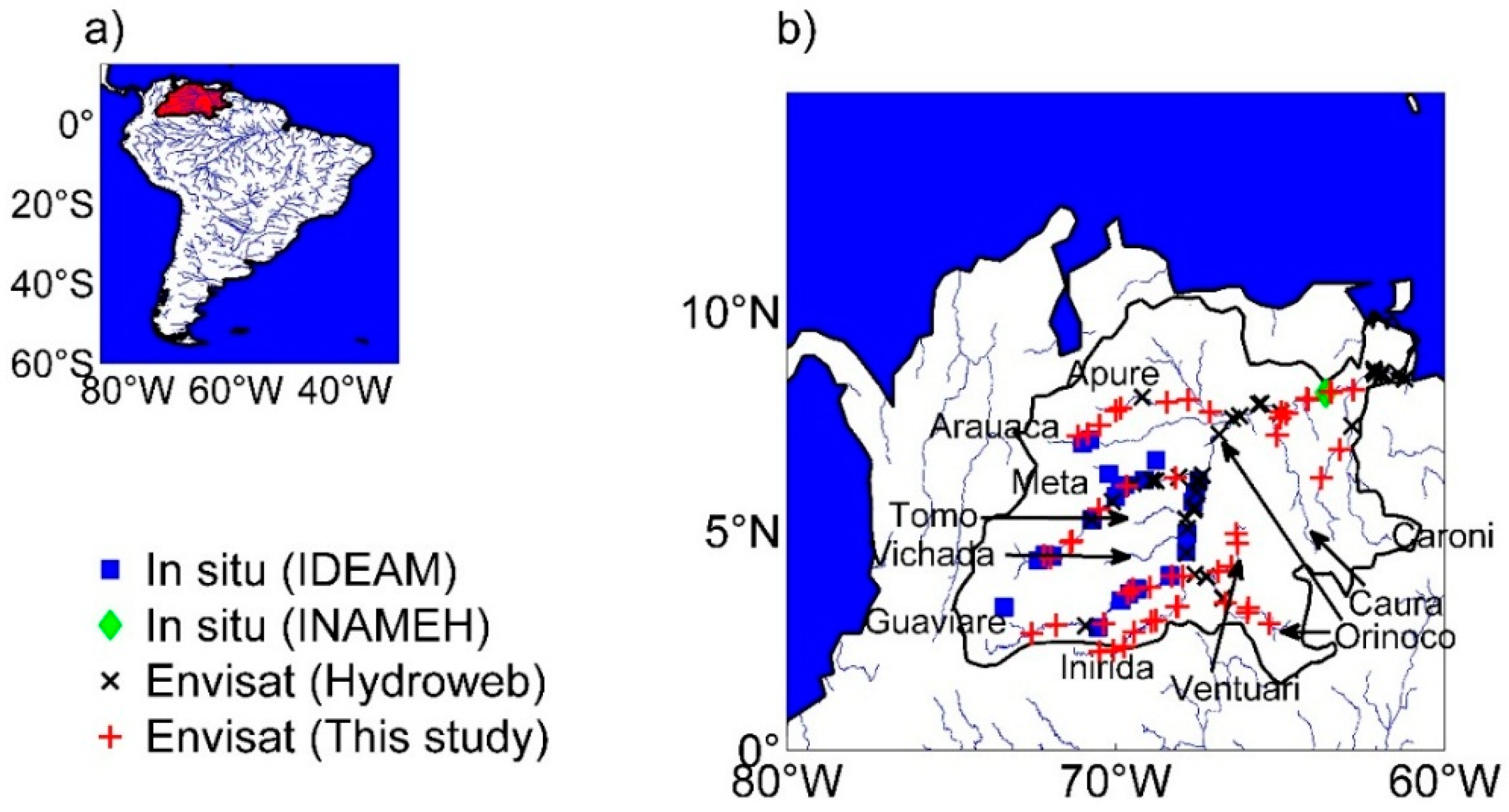
2.1.5. In Situ Water Levels and Discharges

Available in situ hydrometric information corresponded to water levels and, for some cases, to daily flows recorded at 60 stations. These stations are part of the network of the Institute of Hydrology, Meteorology and Environmental Studies of Colombia (IDEAM), which is in charge of monitoring the main channels of the Orinoco Basin in Colombia, including the main channel of the Orinoco, Arauca, Meta, Vichada, Guaviare and Inirida Rivers. Water stages were measured by both limnimetric and limnigraphic stations between March 2002, and October 2010 (the period for which radar altimetry information is available). Of the 60 gauging stations, only 25 stations recorded water levels during the Envisat repetitive observation period: two in the Arauca, eight in the Guaviare, two in the Inírida, 10 in the Meta and three in the Orinoco. In addition, daily water storage and monthly discharge information from 2002 to 2010 for Ciudad Bolivar, close to the mouth of the Orinoco, is made available by the Venezuelan water agency (Instituto Nacional de Meteorologia e Hidrologia, INAMEH). Locations for the in situ stations are shown in Figure 1b and Table 1.
Table 1. List of in situ gauging stations from IDEAM (Colombia) and INAMEH (Venezuela) used for validating altimetry-based water levels during the period of available Envisat data.
In Situ StationRiverLongitude (°)Latitude (°)SourceAvailability during Validation Period
Ciudad BolivarOrinoco−63.6088.144INAMEH2002–2010
Puerto CarrenoOrinoco−67.4676.167IDEAM2002–2010
Puerto NariñoOrinoco−67.8334.950IDEAM2002–2010
RoncadorOrinoco−67.5675.850IDEAM2002–2010
CasuaritoOrinoco−67.6335.667IDEAM2002–2003
MatavenOrinoco−67.8504.533IDEAM2002–2003
Puerto FortunaMeta−68.7676.613IDEAM2002–2010
PatevacalMeta−69.1176.167IDEAM2002–2003
AguaverdeMeta−69.9835.783IDEAM2002–2003
Puerto TexasMeta−71.9174.433IDEAM2002–2003
Santa MariaMeta−70.7175.267IDEAM2002–2010
Peregrino ParaisoMeta−69.7176.050IDEAM2002–2003
San JorgeMeta−69.8506.000IDEAM2002–2003
La PoyataMeta−72.1504.450IDEAM2002–2003
HumapoMeta−72.3504.333IDEAM2002–2003
Cravo NorteMeta−70.2006.300IDEAM2002–2003
Puerto LlerasMeta−73.3833.267IDEAM2002–2008
SapuaraGuaviare−69.3503.683IDEAM2002–2003
Puerto NuevoGuaviare−69.8333.417IDEAM2004–2010
CejalGuaviare−68.3503.983IDEAM2002–2010
MapiripanGuaviare−70.5332.800IDEAM2002–2003
BarrancoGuaviare−69.5893.572IDEAM2003
AngelitosArauaca−71.0007.000IDEAM2002–2005
Ponte InternacionalArauaca−70.7677.083IDEAM2002–2010
Santa RitaVichada−67.9834.867IDEAM2003–2010

2.2. Methods for Estimating Surface Water Storage

The method used to estimate surface freshwater storage consisted of the combination of the surface water extent from GIEMS (Section 2.1.1) with altimeter-derived water level heights estimated at 83 virtual stations (Section 2.1.2). We used both datasets during their period of common availability, from 2003 to 2007. Details of the two-step methodology have been published in [28,62] and are summarized below.

2.2.1. Monthly Maps of Surface Water Levels

Monthly maps of water level in the Orinoco Basin were generated by combining the observations from GIEMS and Envisat RA-2-derived water levels. Following Frappart et al. [27,62], water levels for a given month were linearly interpolated over GIEMS inundation. Each monthly map of surface water levels had a spatial resolution of 0.25°, and the elevation of each pixel was provided with reference to a map of minimum water levels estimated for the entire observation period (2003–2007) using a hypsometric approach (see Frappart et al. [28,29]). The hypsometric approach permitted us to account for the difference of elevation in each cell area of the multi-satellite inundation dataset corresponding to, for instance, the difference in elevation between the river and the floodplain. For each inundated pixel of coordinates (λj, φj), the minimum elevation hmin during the observation period ΔT for a percentage of inundation α was given as (Equation (4)):
h min ( λ i , ϕ i , α , Δ T ) = min ( h ( λ i , ϕ i , t ) ) P ( λ i , ϕ i , t ) α ; t Δ T
where α varies between 0 and 100 and t is a monthly observation during ΔT. The error on these estimates was lower than 10% [27,62].

2.2.2. Time Series of Water Volume Variations

At the basin scale, the time variations of surface water volume are simply computed as described by Frappart et al. [55] (Equation (5)):
V S W ( t ) = R e 2 j S P ( λ j , ϕ j , t ) ( h ( λ j , ϕ j , t ) h min ( λ j , ϕ j , P ( λ j , ϕ j , t ) ) ) cos ( ϕ j ) Δ λ Δ ϕ
where VSW is the volume of surface water, Re is the radius of the Earth (6378 km), P(λj, φj, t), h(λj, φj, t) and hminj, φj) are, respectively, the percentage of inundation and the water level at time t and the minimum water level of the pixel at coordinates (λj, φj). Δλ and Δφ are, respectively, the grid steps in longitude and latitude. This minimum of water level is estimated through a hypsometric approach relating the percentage of inundation of a pixel to its elevation.
Accordingly, the time variations of the volume of terrestrial water storage (TWS) anomalies from GRACE regional solutions [53] are computed following Ramillien et al. [63] (Equation (6)):
Δ V T W S ( t ) = R e 2 j S Δ h t o t ( λ j , ϕ j , t ) cos ( ϕ j ) Δ λ Δ ϕ
where htotj. φj.t) is the anomaly of TWS at time t for the pixel at coordinates (λj, φj).
The error of the method was estimated following Frappart et al. [27,62] (Equation (7)):
d V S W ( t ) = j S ( ( h ( λ j , φ j , t ) h min ( λ j , φ j , P ( λ j , φ j , t ) ) ) d S ( λ j , φ j , t ) + S ( λ j , φ j , t ) d h ( λ j , φ j , t ) )
where dVSW is the error on the surface water volume variation, S(λj, φj, t) is the j-th elementary surface and dS(λj, φj, t) is the error on the j-th elementary surface.
The maximum error for the volume variation can be estimated as (Equation (8)):
max(∆V) = δhmaxSmax + Smaxδhmax
where ∆V is the maximum error on the surface water volume variation, Smax is the maximum flooded surface, δhmax is the maximum water level variation between two consecutive months, ∆Smax is the maximum error for the flooded surface and ∆δhmax is the maximum error for the water level variation between two consecutive months.

3. Results

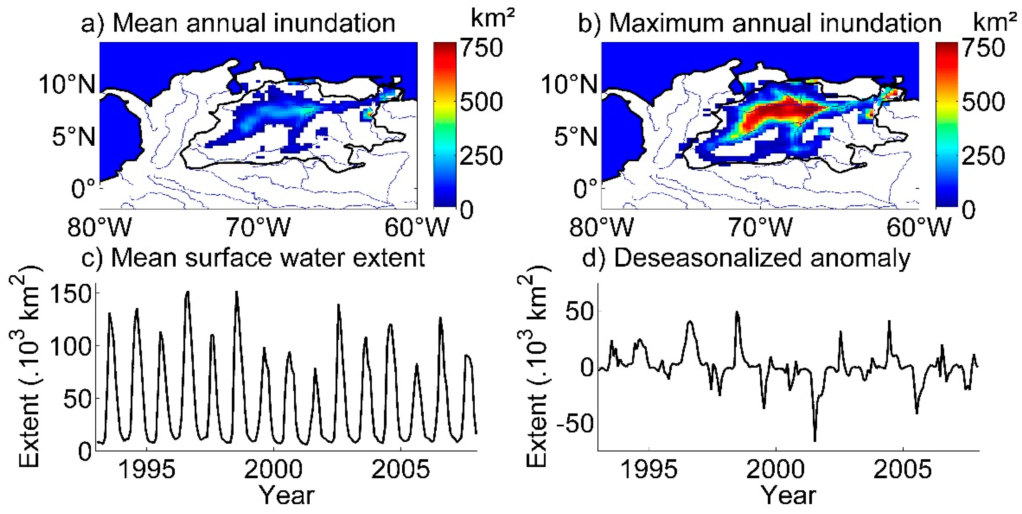
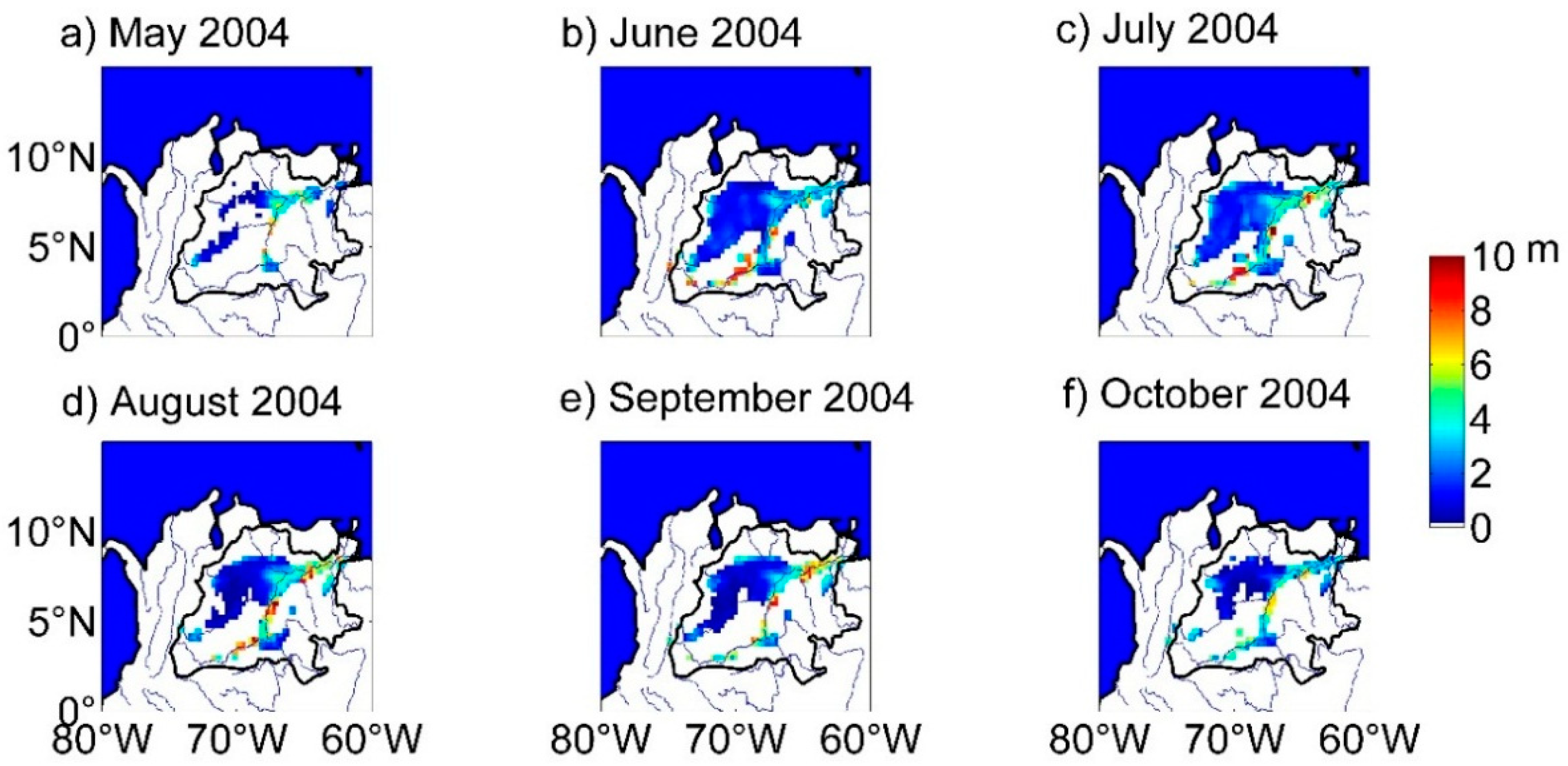
3.1. Temporal Variations of Flood Extent

The time variations of inundation extent were analyzed using GIEMS at a monthly time scale from 1993 to 2007. Figure 2 shows the mean and maximum annual extent of inundation for the Orinoco Basin. Spatial patterns of flooding were very realistic, located along the Orinoco and its major tributaries. Maxima were located in three regions: (i) the Llanos del Orinoco or internal deltaic floodplain, located between the Meta and Apure Rivers between 72°W and 66°W and 4°N and 10°N; (ii) the fringing floodplain along the Orinoco main stem, between 66°W and 62.5°W; and (iii) in the delta between 62°W and 61.5°W and between 8°N and 10°N.
Our results agreed well with previous field observations [33] and with the 37-GHz polarization difference observed by the Scanning Multichannel Microwave Radiometer (SMMR) on the Nimbus-7 satellite [21,22]. The large and permanent open water areas (with constant annual inundation extent) corresponded with Maracaibo lake (the largest lake in South America, with an area of 13,210 km2, centered at 71.56°W and 9.82°N, just outside the boundary of the Orinoco Basin) and Gui reservoir (one of the largest artificial reservoirs in the world, with an area of 4250 km2, constructed on the Caroni River, centered at 63°W and 7°N).
Figure 2. Inundation extent from Global Inundation Extent Multi-Satellite (GIEMS) and anomalies over the Orinoco Basin. Maps of annual mean (a) and annual maximum (b) surface water extent averaged over 1993–2007 for each 773-km2 pixel. (c) Monthly mean surface water extents for 1993–2007 for the entire Orinoco Basin. (d) Corresponding deseasonalized anomalies obtained by subtracting the 15-year mean monthly value from individual months.
Remotesensing 07 00089 g002
Seasonal and interannual variations in surface water extent and associated anomalies over the Orinoco Basin are presented in Figure 2c,d, respectively. The flooded areas exhibited a clear seasonal cycle (Figure 2c), varying from 6000 km2 during low water to 150,000 km2 during high water over the 1993–2007 period. The floods generally occurred between June and October. These values agreed well with previous estimates for the 1980s [21,22,33]. Time variations of flood extent showed a substantial interannual variability that was clearly apparent from the deseasonalized anomalies (Figure 2d). Deseasonalized anomalies were computed as the difference between the flood extent during one month and the average flood extent for the month over the whole observation period. Larger floods occurred in 1993, 1994, 1996, 1998, 2002 and 2006, whereas droughts occurred in 1997, 1999 to 2001 and 2005. Most floods and droughts were related to large El Niño/Southern Oscillation (ENSO) events. Over northeastern South America, El Niño events (positive anomalies of the ENSO index) generally cause droughts, whereas La Niña events (negative anomalies of the ENSO index) are usually responsible for floods [64]. Our observations followed those characteristics, other than for the exceptional drought of 2005, which mostly was caused by an increase of the sea surface temperature (SST) in the tropical North Atlantic [65]. In the case of the historic 1997/1998 ENSO event, a similar succession of positive and negative anomalies of flood extent was observed in the GIEMS dataset over the Negro River Basin, one of the largest tributaries to the Amazon, that shares a common border with the Orinoco Basin [27].

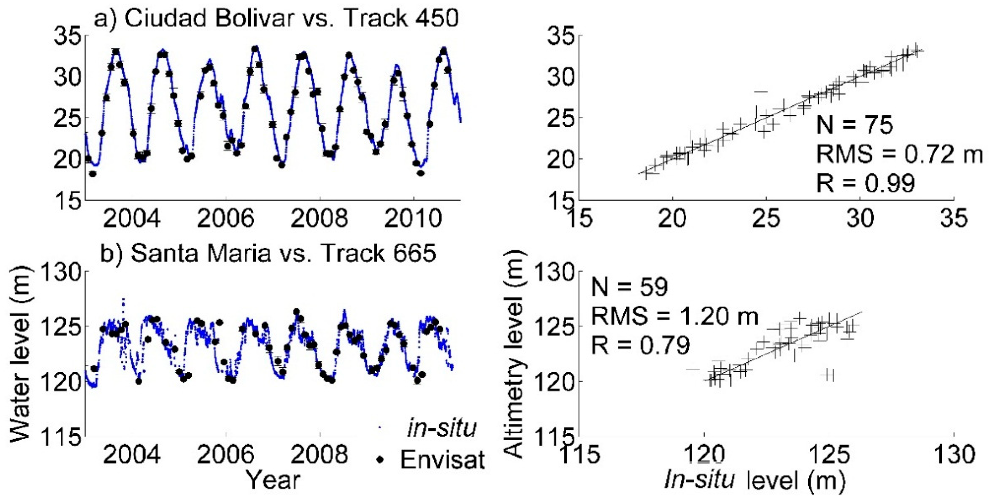
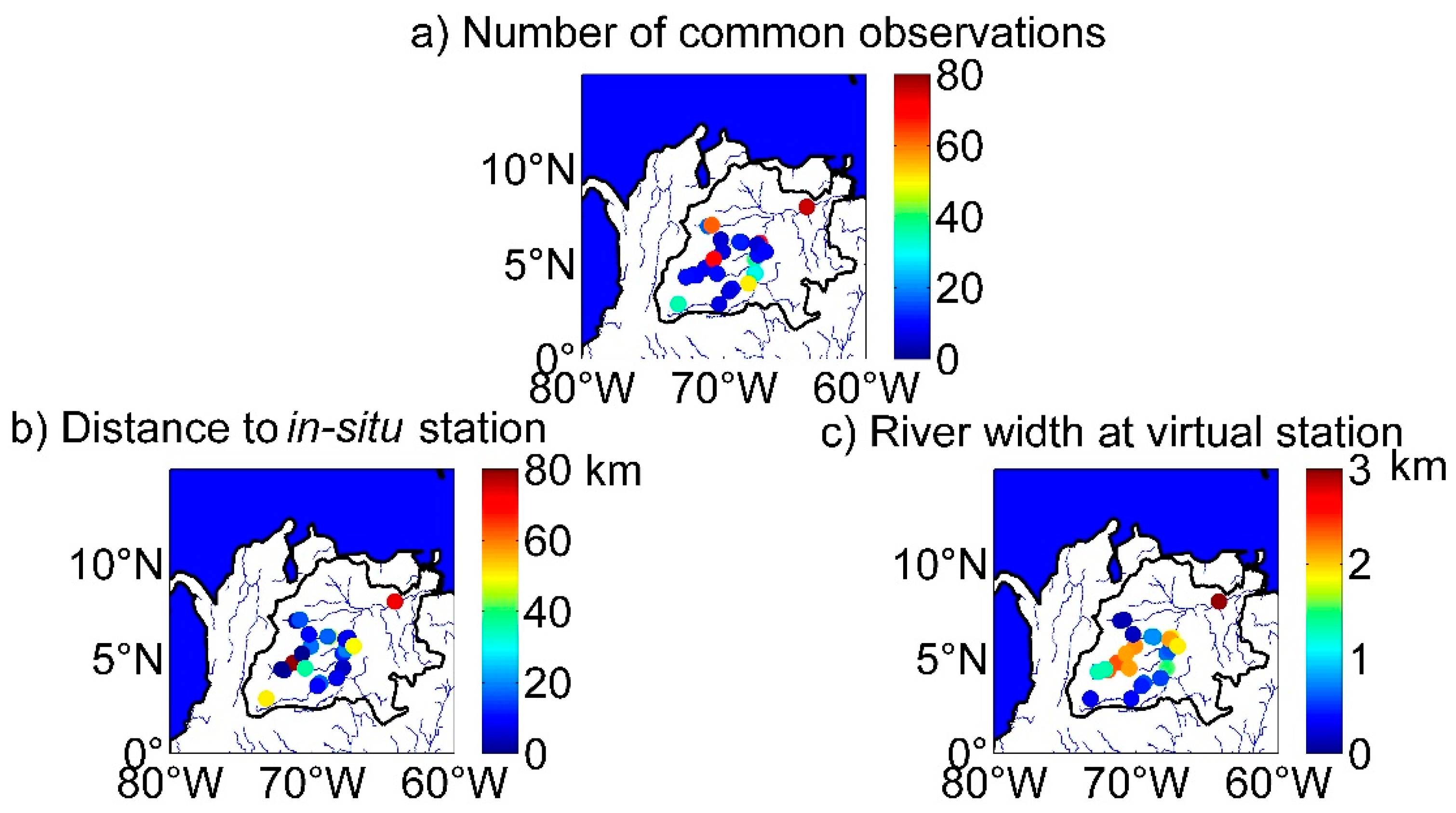
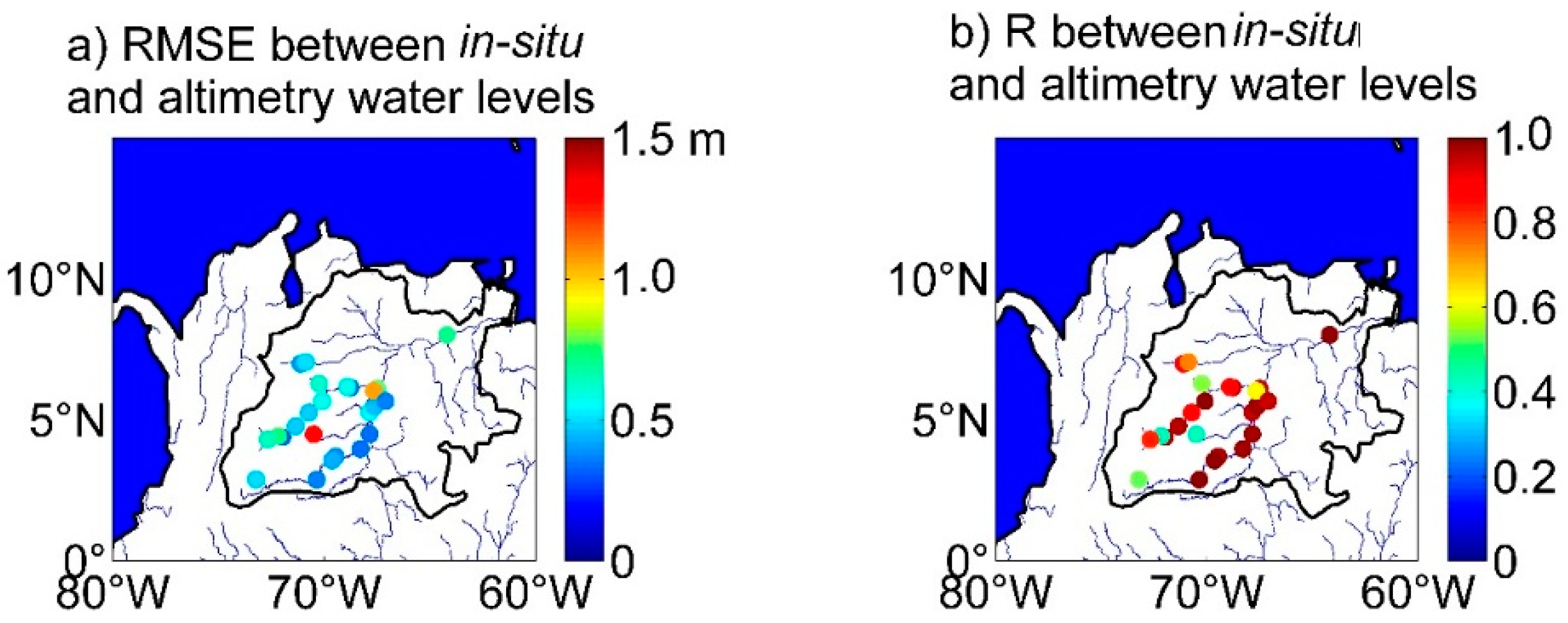
3.2. Validation of Altimetry-Based Water Levels

The quality of altimetry-based water levels was assessed by comparison with in situ measurements from gauges. We used records from 26 gauging stations to perform 28 comparisons, through the comparison of each in situ gauge with the respective upstream and downstream virtual stations. Comparisons between time series of water levels derived from Envisat radar altimetry with in situ gauge records over 2003–2010 for Track 450 at ~74 km upstream from the Ciudad Bolivar gauge (INAMEH) and for Track 665 for the Santa Maria gauge (IDEAM) are shown in (Figure 3). These two examples reflect the large variability of hydrological conditions in the Orinoco Basin from upstream (Santa Maria, in the Meta tributary) to downstream (Ciudad Bolivar, close to the mouth of the Orinoco). For these two cases, altimetry-based water levels exhibited very realistic temporal variations that permitted monitoring of the hydrological cycle. Annual cycles, with variations up to 15 m in Ciudad Bolivar, were consistent across years, along with smaller fluctuations at the monthly time scale. Greater variability in annual cycles was observed at Santa Maria. Simultaneous observations at Ciudad Bolivar (75 observations) and Santa Maria (59 observations), respectively, produced RMSEs of 0.72 m and 1.20 m and correlation coefficients of 0.99 and 0.79.
Figure 3. Two examples of water levels derived from Envisat radar altimetry and compared with in situ gauge records over 2003–2010. (a) Track 450 at ~74 km upstream from the Ciudad Bolivar gauge (INAMEH); (b) Track 665 for the Santa Maria gauge (IDEAM). In both cases, time series of water levels are presented on the left and the corresponding scatterplots on the right.
Remotesensing 07 00089 g003
Similar comparisons were performed for 28 virtual stations. Maps of RMSE and R between altimetry-based and in situ water levels are presented in Figure 4. Overall good agreement was observed between the two datasets with an RMSE lower than 60 cm in more than 75% of the cases and R higher than 0.7 in more than 80% of the comparisons. These results confirm the strong capacity of radar altimetry for retrieving realistic water levels in large drainage basins, as has been shown previously, for example, using ENVISAT in the Orinoco Basin over shorter time periods [66,67].
Figure 4. Comparisons between altimetry-based and in situ water levels over the Orinoco Basin. (a) RMSE (m), (b) R.
Remotesensing 07 00089 g004
Several factors are likely to impact the quality of the estimated water levels based on altimetry measurements, including the topography of the study area, the river width, the vegetation cover and, more generally, the nature and the complexity of the environment encompassed in the footprint (i.e., in a radius of several kilometers, radar altimeter echoes contain reflections not only from open water, but also eventually from bare soils, fields and pastures, cities, roads and bridges, even if the specular reflection from open water dominates the returned power), among others. The validation of the altimetry-derived water levels was often achieved through comparisons with records from nearby gauges. This validation process was highly dependent on the length of the concomitant observations and on the distance to the closest gauge. Previous studies demonstrated the capability of radar altimetry to retrieve reliable water levels over water bodies larger than 200 or 300 m across [46,51,68,69], even over floodplains covered with vegetation [19,68,70]. At nadir incidence, the intensity of the returned power is weakly attenuated by the vegetation cover (at least for Leaf Area Index < 1.5; see [71]), even if the radar echo is impacted.
We analyzed the impact of three factors on the validation process: the number of concomitant observations, the distance between the virtual and the in situ stations and the river width at the location of the virtual station (Figure 5). In more than 60% of the cases, the number of concomitant data was lower than 15. This illustrates the importance of altimetry-based water stages to study the hydrological cycle in the Orinoco Basin. Nevertheless, the distance between the virtual and in situ stations was less than 20 km in 60% of the cases (and less than 10 km in 40% of the cases). This explained the overall good agreement presented in Figures 5, despite the relative narrowness of the river crossings at the locations of the virtual stations. Around 60% of the virtual stations were located on rivers narrower than 1 km and 35% on rivers narrower than 0.5 km. We were able to retrieve a consistent time series of water levels for a crossing of approximately 120 m in width between the Arauca River and Envisat track Number 336. The RMSE and R between the altimetry-based time series of water levels and those from Ponte Internacional were 0.51 m and 0.55 m, respectively. The performances of altimetry-based water levels compared with in situ gauges remained low (RMSE > 0.5 m and R < 0.65) in four cases (15% of all of the comparisons). One or more factors could account for these discrepancies. Very few in situ data (between six and 10 stations) were available for comparisons in three of these four cases. In two cases, the river width at the location of the virtual station was less than 300 m. In two other cases, the distance between virtual and in situ stations was greater than 35 km, so local hydrological effects, such as rain events, presence of tributaries, variations in width and presence of sandbanks, especially in the upstream part of the basin, could have altered the temporal variations recorded at the two locations.
Figure 5. Comparisons between altimetry-based and in situ water levels over the Orinoco Basin. (a) Number of common observations; (b) distance between virtual and in situ stations (km); (c) river width at virtual station.
Remotesensing 07 00089 g005

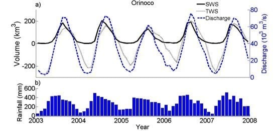
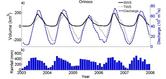
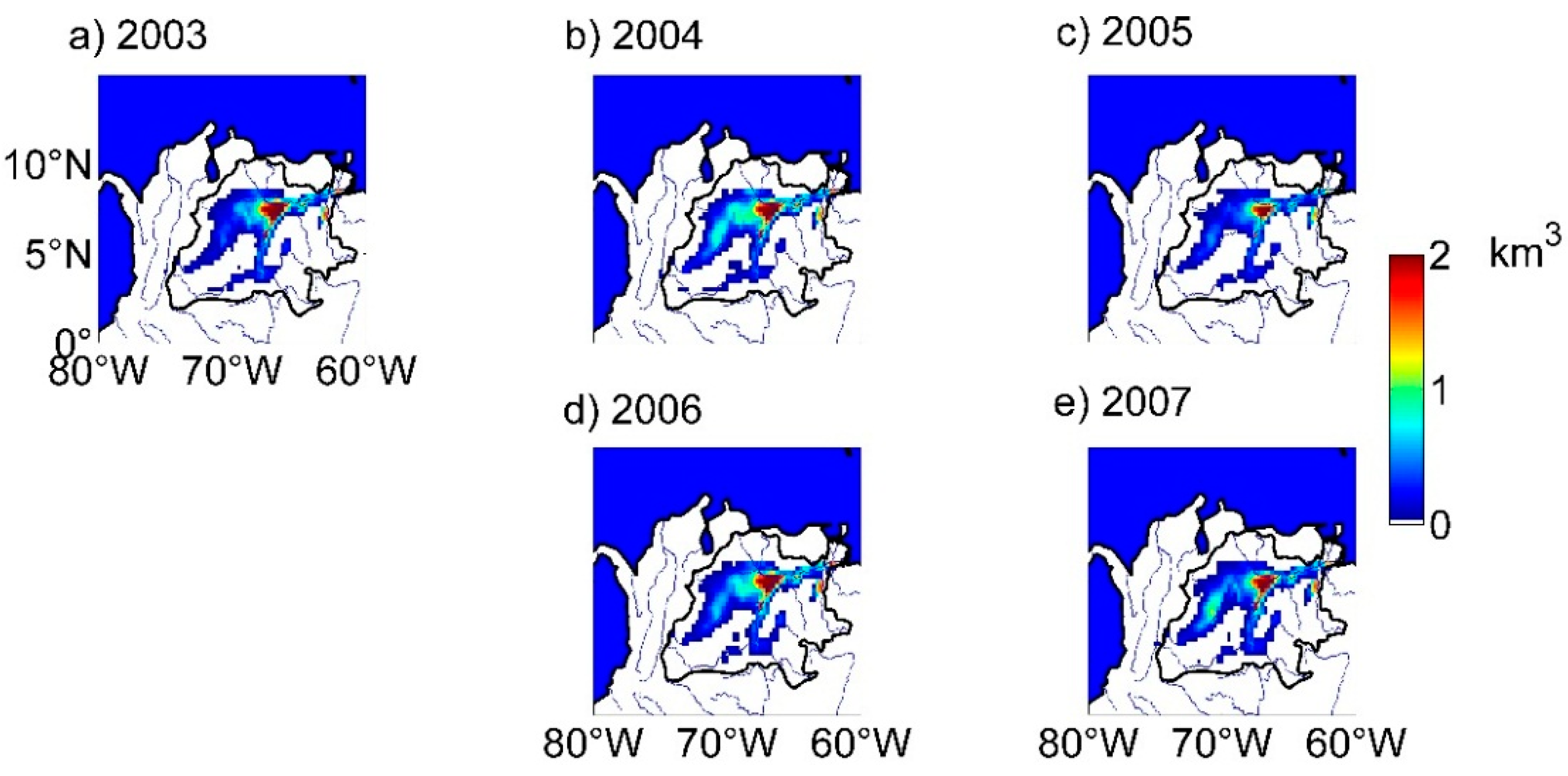
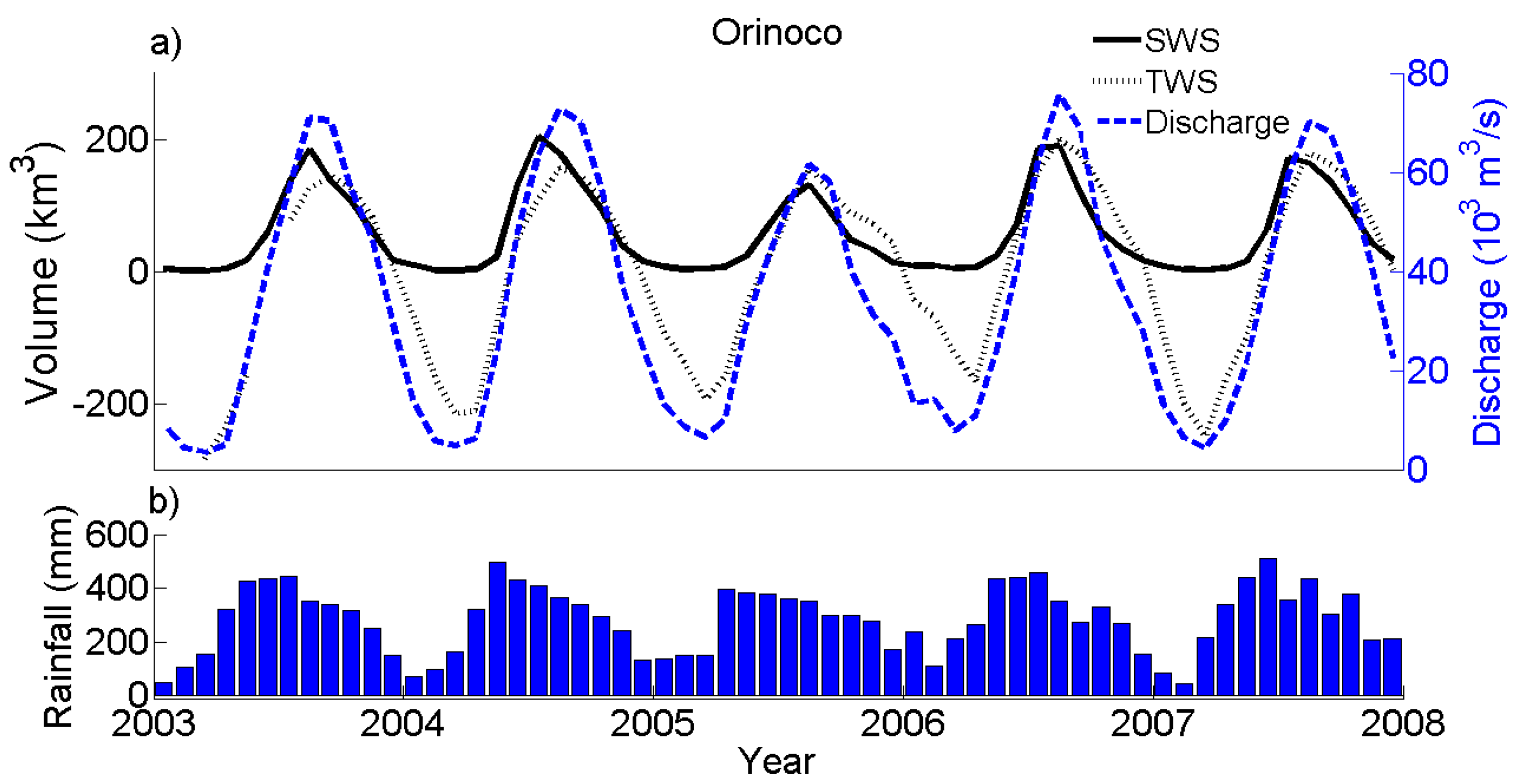
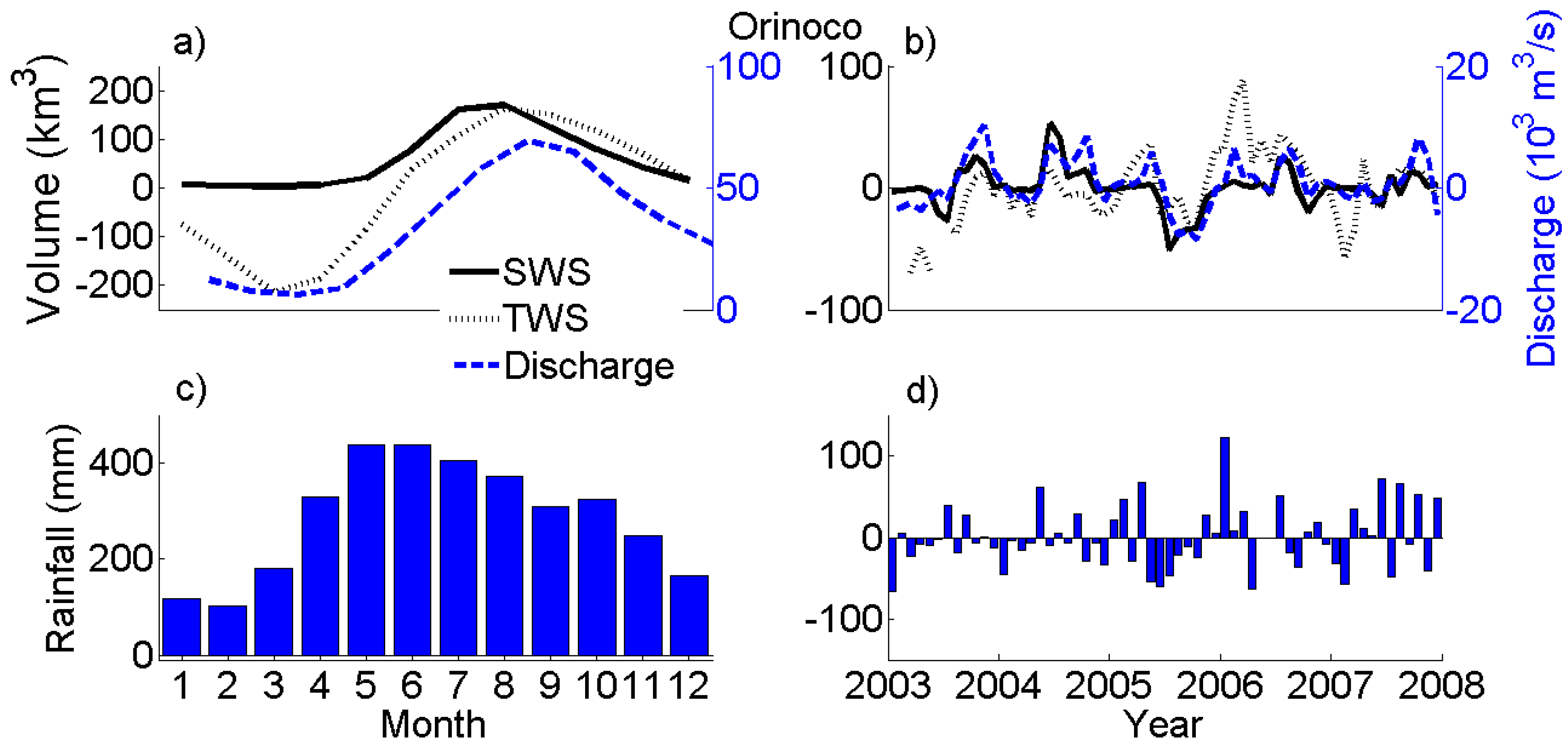
3.3. Time Variations of Surface Water Storage in the Orinoco Floodplains

Prior to calculating the surface water storage over the full basin, it was necessary to interpolate the sparse water levels provided by the altimeter to the whole inundated area following the approach described in Section 2.2.1. Monthly maps of surface water levels were computed by combining multi-satellite-based inundation maps from GIEMS with 83 Envisat altimetry-derived water levels in the Orinoco Basin. Seasonal variations of water levels are presented in Figure 6 for May to October 2004. They allowed us to monitor the flood pulse in the Orinoco Basin. In 2004, the flood started in May in the western part of the basin, with small inundation in the upstream part of the Meta and Apure Rivers (Figure 6a). Maximum flooding of upstream areas was characterized by large inundation of small amplitude (below 2 m) in the inner delta between the Meta and the Apure Rivers and at junctions between the Orinoco and the Guaviare, Inirida and Ventuari Rivers. The flood pulse propagated toward the mouth of the Orinoco in June and July (Figure 6b,c). Subsequently, the flood started to decline in the upstream parts of the basin, while reaching its maximum in the fringing floodplain along the main stem of the Orinoco and in the delta (Figure 6d), followed by decline across the whole basin (Figure 6d,e). These seasonal variations exhibited very consistent patterns when compared with previous studies on inundation extent and water stages in the Orinoco Basin [21,22,33].
Figure 6. Monthly maps of water levels from altimetry spatially extended with GIEMS for (a) May, (b) June, (c) July, (d) August, (e) September and (f) October 2004.
Remotesensing 07 00089 g006
These monthly maps of water levels were used to estimate surface water storage expressed as volumes for 2003–2007. Spatial patterns of surface storage changes, computed as the difference between the maximum and the minimum surface water storage during the year, are presented over 2003–2007 in Figure 7. The spatial patterns are very realistic along the Orinoco River and its major tributaries, as well as in the inner delta region. The delta region presented very low storage changes, as variations in water levels are very low. Maximum storage changes occurred in the downstream part of the inner delta region, reaching 2 km3/year per grid cell at the confluences of the Meta and Apure Rivers with the Orinoco. Secondary maxima were also observed in 2004, 2006 and 2007 in the inner delta along the Arauca River (Figure 7b,d,e), with changes around 0.75–1 km3/year.
Figure 7. Surface water storage variations between minimum and maximum water stages in the Orinoco Basin from GIEMS and altimetry for (a) 2003, (b) 2004, (c) 2005, (d) 2006 and (e) 2007.
Remotesensing 07 00089 g007
In terms of time variations, surface water storage exhibited a strong seasonal signal, generally peaking in July or August (Figure 8). Rainfall increases were followed by increased surface water storage (R = 0.87) with a time-lag of two months (Figure 8). Surface water storage was highly correlated with river flow (R = 0.95, with the record of the Ciudad Bolivar gauge, the last station along the Orinoco main stem where discharge data were available) and preceded it by one month. Lower correlation was found with TWS (R = 0.62 for a time-lag of one month), suggesting that other hydrological reservoirs, such as sub-surface and groundwater, also had a strong influence on TWS.
Figure 8. Time series of (a) surface water storage (SWS) from altimetry and imagery (black line), the total water storage (TWS) anomaly from Gravity Recovery and Climate Experiment (GRACE) regional solutions in the Orinoco Basin (dotted black line) and discharge at Ciudad Bolivar (dashed blue line); (b) rainfall from TRMM 3B43 v7 over 2003–2007.
Remotesensing 07 00089 g008
We estimated the maximum error for the volume change in the floodplains of the Orinoco Basin using Equation (8) and the following values:
Smax = 120,000 km2 in August, 2004; δhmax = 1 m, mean maximum water level change between two consecutive months during the study period over the whole area;
ΔSmax = 10% from [24] of 120,000 km2; and Δδhmax = 0.4 m, maximum average dispersion of the altimeter measurements over the whole area in 2004.
We obtained a maximum error of 60 km3 for an annual variation of 200 km3 in 2004, i.e., an error of ~30%. This is of the same order of magnitude as the maximum error (23%) found for the Rio Negro in the Amazon Basin [27,62].
The mean annual amplitude of surface water storage was around 170 km3 for an average annual basin-wide rainfall of ~3450 mm from 2003 to 2007 (Figure 9a,c). Surface water storage represented about 13% of the total volume of water that flowed out of the Orinoco Basin to the Atlantic Ocean and contributed to 45% of the annual changes in TWS as measured by GRACE (~380 km3).
Surface water storage exhibited a large interannual variability over 2003–2007 (Figure 9b, R = 0.73 for a time-lag of one month), similar to that observed for river discharge. The deseasonalized surface storage presented a positive anomaly larger than 50 km3 in June, 2004, and a negative anomaly of ~50 km3 in July 2005 (Figure 9b). The positive anomaly of 2004 was caused by warmer conditions in the Central Pacific responsible for a small increase in rainfall in a three-year period of low rainfall due to low and moderate El Niño events [72]. The negative anomaly of 2005 was attributable to a long dry spell caused by the moderate ENSO phenomenon of 2002–2003 and an increase of sea surface temperature in the subtropical North Atlantic Ocean [65,72] (see Figure 9d). This coincided with the extreme drought of 2005 in the Amazon Basin (see, for example, its effect on surface water storage and TWS in the Amazon basin [11,28]). The large positive anomaly in rainfall at the end of 2005 and the beginning of 2006 did not cause large floods in winter 2006, but replenished the different hydrological reservoirs that were strongly impacted by the 2005 drought; however, the rainfall anomaly was responsible for the peak in TWS observed in 2006 (Figure 9b). Similar observations were made in the Amazon basin for 2006 [11,61].
Figure 9. (a) Annual cycles and (b) deseasonalized variations of surface water storage (SWS) from altimetry and imagery (black line), the total water storage (TWS) anomaly from GRACE regional solutions in the Orinoco Basin (dotted black line) and discharge at Ciudad Bolivar (dashed blue line). (c) Annual cycle and (d) deseasonalized variations of rainfall TRMM 3B43 v7 over 2003–2007.
Remotesensing 07 00089 g009

4. Summary and Conclusions

This study presents an analysis of the surface water extent (1993–2007) and storage (2003–2007) in the floodplains of the Orinoco Basin at a spatial resolution of ~25 km. We used satellite-based products to quantify the monthly distribution and variation of surface freshwater extent from the GIEMS dataset (e.g., [24,26,42]) and freshwater storage from a new product based on the combination of surface water extent from GIEMS and inland water stages from Envisat radar altimetry following the approach proposed earlier by Frappart et al. [28]. A total of 83 time series of water level variations were constructed using Envisat radar altimeter observations. These altimeter-based water stages were validated through direct comparisons with in situ river levels from Colombian (IDEAM) and Venezuelan (INAMEH) water agencies, confirming the high efficiency of radar altimetry for monitoring inland water bodies.
Annual floods generally occurred from June to October and covered between 80,000 and 150,000 km2 at their maxima for the period 1993–2007. Their large interannual variability was mostly related to ENSO phenomena. Surface water storage estimates exhibited very realistic spatial and temporal patterns when compared with existing information, such as rainfall, discharges and TWS. High temporal correlations were found with rainfall (R = 0.87) and discharge (R = 0.95), and a relatively lower correlation was found with TWS (R = 0.62). Temporal patterns of TWS lagged two months behind temporal patterns of rainfall; similarly, discharge lagged one month behind storage. These time lags can be attributed to the exchange of water between the surface reservoir and the subsurface and groundwater reservoirs and their slower flow in comparison to surface water movement. Surface water storage also presented large annual cycles and a strong interannual variability (e.g., the drought of 2005). Mean annual variation in surface water storage was around 180 km3 and contributed to 45% of the annual variations of TWS and 15% of the annual volume that flowed from the Orinoco River to the Atlantic Ocean.
Maps of surface water storage are a new and unique product for the evaluation of: (i) surface reservoir estimates from regional and global hydrological models, especially over floodplains where data are scarce; and (ii) subsurface and groundwater storage by directly removing the surface component of the TWS. The maps are informative about changes affecting the hydrological cycle in large river basins with extensive floodplains and to improve our understanding of the complex dynamics of surface water in large drainage basins (i.e., backwater effects, the flood-pulse linked to the strong seasonality of the rainfall and the residence time of water in the floodplains). The products will be extended temporally using data from former (ERS-1 and 2) and current (SARAL) altimetry missions that were/are on the same orbit or in combination with data from other altimetry missions (Topex/Poseidon, Geosat Follow-On, Jason-2, Jason-3, Sentinel-3A, etc.). In addition, the estimation of the surface water storage can be used to subtract the surface water component of the TWS and isolate the subsurface and groundwater components. The products offer a unique opportunity to continuously monitor mass transport in the surface water reservoir before the launch of the NASA-CNES Surface Water and Ocean Topography (SWOT) mission in 2020.

Acknowledgments

This work is supported by the CNES-TOSCA, OST-ST “Variability of terrestrial freshwater storage in the Tropics from multi-satellite observations” and “From Ocean to inland waters Altimetry Monitoring” (FOAM) and by ECOS Nord “C12U02” grants. We thank three anonymous reviewers for their helpful comments and guest editor Dr. Alisa L. Gallant for helping us with improving the quality of the manuscript.

Author Contributions

All of the authors of the present work contributed to the discussion of the results, as well as the writing of the manuscript. Frédéric Frappart and Fabrice Papa designed the study. Frédéric Frappart, Fabrice Papa and Yoann Malbeteau analyzed and discussed the preliminary results. Fabrice Papa and Catherine Prigent provided the Global Inundation Extent from Multi-Satellites (GIEMS) dataset, and Guillaume Ramillien and Lucía Seoane provided the GRACE regional solutions. Juan Gabriel León, Yoann Malbeteau, Frédérique Seyler and Stéphane Calmant performed the validation of Envisat RA-2 altimetry-based water levels.

Conflicts of Interest

The authors declare no conflicts of interest.

References

  1. Chahine, M. The hydrological cycle and its influence on climate. Nature 1992, 359, 373–380. [Google Scholar] [CrossRef]
  2. Kundzewicz, Z.W.; Mata, L.J.; Arnell, N.W.; Döll, P.; Kabat, P.; Jiménez, B.; Miller, K.A.; Oki, T.; Sen, Z.; Shiklomanov, I.A. Freshwater resources and their management. In Climate Change 2007: Impacts. Adaptation. and Vulnerability. Contribution of Working Group II to the Fourth Assessment Report of the Intergovernmental Panel on Climate Change; Parry, M.L., Canziani, O.F., Palutikof, J.P., van der Linden, P.J., Hanson, C.E., Eds.; Cambridge University Press: Cambridge, UK, 2007; pp. 173–210. [Google Scholar]
  3. Maltby, E. Wetland management goals: Wise use and conservation. Landsc. Urban Plan. 2003, 20, 9–18. [Google Scholar] [CrossRef]
  4. Bullock, A.; Acreman, M. The role of wetlands in the hydrological cycle. Hydrol. Earth Syst. Sci. 2003, 7, 358–389. [Google Scholar] [CrossRef]
  5. Organisation for Economic Cooperation and Development. Guidelines for Aid Agencies for Improved Conservation and Sustainable Use of Tropical and Sub-tropical Wetlands; Guidelines Aid Environment: Paris, France, 1996. [Google Scholar]
  6. Richey, J.E.; Melack, J.M.; Aufdenkampe, K.; Ballester, V.M.; Hess, L. Outgassing from Amazonian rivers and wetlands as a large tropical source of atmospheric CO2. Nature 2002, 416, 617–620. [Google Scholar] [CrossRef] [PubMed]
  7. Bousquet, P.; Ciais, P.; Miller, J.B.; Dlugokencky, E.J.; Hauglustaine, D.A.; Prigent, C.; van der Werf, G.R.; Peylin, P.; Brunke, E.-G.; Carouge, C.; et al. Contribution of anthropogenic and natural sources to atmospheric methane variability. Nature 2006, 443, 439–443. [Google Scholar] [CrossRef] [PubMed]
  8. Ringeval, B.; de Noblet-Ducoudré, N.; Ciais, P.; Bousquet, P.; Prigent, C.; Papa, F.; Rossow, W.B. An attempt to quantify the impact of changes in wetland extent on methane emissions at the seasonal and interannual time scales. Glob. Biochem. Cy. 2010, 24. [Google Scholar] [CrossRef]
  9. Decharme, B.; Douville, H.; Prigent, C.; Papa, F.; Aires, F. A new river flooding scheme for global climate applications: Off-line validation over South America. J. Geophys. Res. 2008, 113. [Google Scholar] [CrossRef]
  10. Azarderakhsh, M.; Rossow, W.B.; Papa, F.; Norouzi, H.; Khanbilvardi, R. Diagnosing water variations within the Amazon basin using satellite data. J. Geophys. Res. 2011, 116. [Google Scholar] [CrossRef] [Green Version]
  11. Frappart, F.; Ramillien, G.; Ronchail, J. Changes in terrestrial water storage versus rainfall and discharges in the Amazon basin. Int. J. Climatol. 2013, 33, 3029–3046. [Google Scholar] [CrossRef] [Green Version]
  12. Paiva, R.C.D.; Buarque, D.C.; Colischonn, W.; Bonnet, M.-P.; Frappart, F.; Calmant, S.; Mendes, C.A.B. Large-scale hydrological and hydrodynamics modelling of the Amazon River basin. Water Resour. Res. 2013, 49, 1226–1243. [Google Scholar] [CrossRef] [Green Version]
  13. Junk, W.J.; Bayley, P.B.; Sparks, R.E. The Flood-Pulse Concept in River-Floodplain Systems. Available online: http://swrcb2.swrcb.ca.gov/waterrights/water_issues/programs/bay_delta/bay_delta_plan/water_quality_control_planning/docs/sjrf_spprtinfo/junk_et_al_1989.pdf (accessed on 29 September 2014).
  14. Richey, J.E.; Mertes, L.A.K.; Dunne, T.; Victoria, R.L.; Forsberg, B.R.; Tancredi, C.; Oliveira, E. Sources and routing of the Amazon River flood wave. Glob. Biogeochem. Cy. 1989, 3, 191–204. [Google Scholar] [CrossRef]
  15. Mertes, L.A.K.; Daniel, D.L.; Melack, J.M.; Nelson, B.; Martinelli, L.A.; Forsberg, B.R. Spatial patterns of hydrology, geomorphology and vegetation on the floodplain of the Amazon River in Brazil from a remote sensing perspective. Geomorphology 1995, 13, 215–222. [Google Scholar] [CrossRef]
  16. Hamilton, S.K.; Sippel, S.J.; Calheiros, D.F.; Melack, J.M. An anoxic event and other biogeochemical effects of the Pantanal wetland on the Paraguay River. Limnol. Oceanogr. 1997, 42, 257–272. [Google Scholar] [CrossRef]
  17. Junk, W.J. The Central Amazon Floodplain: Ecology of a Pulsing System; Springer: Brelin, Germany, 1997. [Google Scholar]
  18. Alsdorf, D.E.; Smith, L.C.; Melack, J.M. Amazon floodplain water level changes measured with interferometric SIR-C radar. IEEE Trans. Geosci. Remote Sens. 2001, 39, 423–431. [Google Scholar] [CrossRef]
  19. Frappart, F.; Seyler, F.; Martinez, J.M.; León, J.G.; Cazenave, A. Floodplain water storage in the Negro River basin estimated from microwave remote sensing of inundation area and water levels. Remote Sens. Environ. 2005, 99, 387–399. [Google Scholar] [CrossRef] [Green Version]
  20. Hamilton, S.K.; Sippel, S.J.; Melack, J.M. Inundation patterns in the Pantanal wetland of South America determined from passive microwave remote sensing. Arch. Hydrobiol. 1996, 137, 1–23. [Google Scholar]
  21. Hamilton, S.K.; Sippel, S.J.; Melack, J.M. Comparison of inundation patterns among major South American floodplains. J. Geophys. Res. 2002, 107. [Google Scholar] [CrossRef]
  22. Hamilton, S.K.; Sippel, S.J.; Melack, J.M. Seasonal inundation patterns in two large savanna floodplains of South America: The Llanos de Moxos (Bolivia) and the Llanos del Orinoco (Venezuela and Colombia). Hydrol. Process. 2004, 18, 2103–2116. [Google Scholar] [CrossRef]
  23. Prigent, C.; Matthews, E.; Aires, F.; Rossow, W.B. Remote sensing of global wetland dynamics with multiple satellite datasets. Geophys. Res. Lett. 2001, 28, 4631–4634. [Google Scholar] [CrossRef]
  24. Prigent, C.; Papa, F.; Aires, F.; Rossow, W.B.; Matthews, E. Global inundation dynamics inferred from multiple satellite observations, 1993–2000. J. Geophys. Res. 2007, 112. [Google Scholar] [CrossRef]
  25. Bourrel, L.; Phillips, L.; Moreau, S. The dynamics of floods in the Bolivian Amazon Basin. Hydrol. Process. 2009, 23, 3161–3167. [Google Scholar] [CrossRef]
  26. Papa, F.; Prigent, C.; Rossow, W.B.; Matthews, E. Interannual variability of surface water extent at global scale. 1993–2004. J. Geophys. Res. 2007, 115. [Google Scholar] [CrossRef]
  27. Frappart, F.; Papa, F.; Famiglietti, J.S.; Prigent, C.; Rossow, W.B.; Seyler, F. Interannual variations of river water storage from a multiple satellite approach: A case study for the Rio Negro River basin. J. Geophys. Res. 2008, 113. [Google Scholar] [CrossRef] [Green Version]
  28. Frappart, F.; Papa, F.; Santos da Silva, J.; Ramillien, G.; Prigent, C.; Seyler, F.; Calmant, S. Surface freshwater storage and dynamics in the Amazon basin during the 2005 exceptional drought. Environ. Res. Lett. 2012, 7. [Google Scholar] [CrossRef] [Green Version]
  29. Papa, F.; Frappart, F.; Güntner, A.; Prigent, C.; Aires, F.; Getirana, A.C.V.; Maurer, R. Surface freshwater storage and variability in the Amazon basin from multi-satellite observations. 1993–2007. J. Geophys. Res. Atmos. 2013, 118, 11951–11965. [Google Scholar] [CrossRef]
  30. Meade, R.H.; Nordin, C.F.J.; Perez Hernandez, D.; Mejia, A.; Perez Godoy, J.M. Sediment and water discharge in Rio Orinoco, Venezuela and Colombia. In Proceedings of the Second International Symposium on River Sedimentation, Beijing, China, 11–16 October 1980.
  31. Silva Leon, G. The Orinoco River Basin: Hydrographic View and Its Hydrological Balance. Available online: http://www.saber.ula.ve/bitstream/123456789/24636/2/articulo4.pdf (accessed on 29 September 2014).
  32. Lewis, W.M., Jr.; Saunders, J.F., III. Concentration and transport of dissolved and suspended substances in the Orinoco River. Biogeochemistry 1989, 7, 203–240. [Google Scholar] [CrossRef]
  33. Hamilton, S.K.; Lewis, W.M., Jr. Physical Characteristics of the Fringing Floodplain of the Orinoco River, Venezuela. Available online: http://ciresweb.colorado.edu/limnology/pubs/pdfs/Pub110.pdf (accessed on 29 September 2014).
  34. Hamilton, S.K.; Lewis, W.M., Jr. Basin Morphology in Relation to Chemical and Ecological Characteristics of Lakes on the Orinoco River Floodplain. Venezuela. Available online: http://cires.colorado.edu/limnology/pubs/pdfs/Pub113.pdf (accessed on 29 September 2014).
  35. Prigent, C.; Papa, F.; Aires, F.; Jimenez, C.; Rossow, W.B.; Matthews, E. Changes in land surface water dynamics since the 1990s and relation to population pressure. Geophys. Res. Lett. 2012, 39. [Google Scholar] [CrossRef]
  36. Papa, F.; Prigent, C.; Durand, F.; Rossow, W.B. Wetland dynamics using a suite of satellite observations: A case study of application and evaluation for the Indian Subcontinent. Geophys. Res. Lett. 2006, 33. [Google Scholar] [CrossRef]
  37. Tucker, C.J. Red and photographic infrared linear combinations for monitoring vegetation. Remote Sens. Environ. 1979, 8, 127–150. [Google Scholar] [CrossRef]
  38. Prigent, C.; Aires, F.; Rossow, W.B. Land surface microwave emissivities over the globe for a decade. Bull. Am. Meteorol. Soc. 2006, 87, 1573–1584. [Google Scholar] [CrossRef]
  39. Rossow, W.B.; Schiffer, R.A. Advances in understanding clouds from ISCCP. Bull. Am. Meteorol. Soc. 1999, 80, 2261–2287. [Google Scholar] [CrossRef]
  40. Kalnay, E.; Kanamitsu, M.; Kistler, R.; Collins, W.; Deaven, D.; Gandin, L.; Iredell, M.; Saha, S.; White, G.; Woollen, J.; et al. The NCEP/NCAR 40-year reanalysis project. Bull. Am. Meteorol. Soc. 1996, 77, 437–470. [Google Scholar] [CrossRef]
  41. Armstrong, R.L.; Brodzik, M.J. Northern Hemisphere EASE-Grid Weekly Snow Cover and Sea Ice Extent Version 3; National Snow and Ice Data Center: Boulder, CO, USA, 2005. [Google Scholar]
  42. Papa, F.; Güntner, A.; Frappart, F.; Prigent, C.; Rossow, W.B. Variations of surface water extent and water storage in large river basins: A comparison of different global data sources. Geophys. Res. Lett. 2008, 35. [Google Scholar] [CrossRef] [Green Version]
  43. Birkett, C.M. The contribution of TOPEX/POSEIDON to the global monitoring of climatically sensitive lakes. J. Geophys. Res. 1995, 100. [Google Scholar] [CrossRef]
  44. Birkett, C.M. Contribution of the TOPEX NASA Radar Altimeter to the global monitoring of large rivers and wetlands. Water Resour. Res. 1998, 34, 1223–1239. [Google Scholar] [CrossRef]
  45. Frappart, F.; Calmant, S.; Cauhopé, M.; Seyler, F.; Cazenave, A. Preliminary results of ENVISAT RA-2 derived water levels validation over the Amazon basin. Remote Sens. Environ. 2006, 100, 252–264. [Google Scholar] [CrossRef] [Green Version]
  46. Frappart, F.; Do Minh, K.; L’Hermitte, J.; Cazenave, A.; Ramillien, G.; Le Toan, T.; Mognard-Campbell, N. Water volume change in the lower Mekong basin from satellite altimetry and imagery data. Geophys. J. Int. 2006, 167, 570–584. [Google Scholar] [CrossRef]
  47. Zelli, C. ENVISAT RA-2 advanced radar altimeter: Instrument design and pre-launch performance assessment review. Acta. Astronaut. 1999, 44, 323–333. [Google Scholar] [CrossRef]
  48. Hydroweb Database. Available online: http://www.legos.obs-mip.fr/en/soa/hydrologie/hydroweb (accessed on 3 January 2013).
  49. Virtual Altimetry Station Software, Version 0.6.2. Available online: www.mpl.ird.fr/hybam/outils/logiciels_test.php (accessed on 5 March 2013).
  50. Center for Topographic Studies of the Ocean and Hydrosphere. Available online: http://ctoh.legos.obs-mip.fr (accessed on 15 March 2013).
  51. Santos Da Silva, J.; Calmant, S.; Seyler, F.; Corrêa Rotunno Filho, O.; Cochonneau, G.; Mansur, W.J. Water levels in the Amazon basin derived from the ERS 2 and ENVISAT radar altimetry missions. Remote Sens. Environ. 2010, 114, 2160–2181. [Google Scholar] [CrossRef]
  52. Pavlis, N.K.; Holmes, S.A.; Kenyon, S.C.; Factor, J.K. The development and evaluation of the Earth Gravitational Model 2008 (EGM2008). J. Geophys. Res. 2012, 117. [Google Scholar] [CrossRef]
  53. Office of Geomatics: World Geodetic System 1984 (WGS 84). Available online: http://earth-info.nga.mil/GandG/wgs84/ (accessed on 15 March 2013).
  54. Tropical Rainfall Measuring Mission (TRMM) 3B43 v7 Product. Available online: http://disc.sci.gsfc.nasa.gov/precipitation/documentation/TRMM_README/TRMM_3B43_readme.shtml (accessed on 1 September 2014).
  55. Huffmann, G.J.; Adler, R.F.; Rudolf, B.; Schneider, U.; Keehn, P.R. Global precipitation estimates based on a technique for combining satellite-based estimates rain gauge analysis and NWP model precipitation information. J. Clim. 1995, 8, 1284–1295. [Google Scholar] [CrossRef]
  56. Huffmann, G.J.; Adler, R.F.; Bolvin, D.T.; Gu, G.; Nelkin, E.J.; Bowman, K.P.; Hong, Y.; Stocker, E.F.; Wolf, D.B. The TRMM multi-satellite precipitation analysis (TMPA): Quasi-global. multi-year combined-sensor precipitation estimates at fine scale. J. Hydrometeorol. 2007, 8, 38–55. [Google Scholar] [CrossRef]
  57. Goddard Earth Sciences Data and Information Services Center (GES DISC). Available online: http://daac.gscf.nasa.gov (accessed on 1 September 2014).
  58. Tapley, B.D.; Bettadpur, S.; Watkins, M.; Reigber, C. The gravity recovery and climate experiment: Mission overview and early results. Geophys. Res. Lett. 2004, 31. [Google Scholar] [CrossRef]
  59. Ramillien, G.; Biancale, R.; Gratton, S.; Vasseur, X.; Bourgogne, S. GRACE-derived surface mass anomalies by energy integral approach. Application to continental hydrology. J. Geodesy 2011, 85, 313–328. [Google Scholar] [CrossRef]
  60. Ramillien, G.; Seoane, L.; Frappart, F.; Biancale, R.; Gratton, S.; Vasseur, X.; Bourgogne, S. Constrained regional recovery of continental water mass time-variations from GRACE-based geopotential anomalies over South America. Surv. Geophys. 2012, 33, 887–905. [Google Scholar] [CrossRef] [Green Version]
  61. Frappart, F.; Seoane, L.; Ramillien, G. Validation of GRACE-derived water mass storage using a regional approach over South America. Remote Sens. Environ. 2013, 137, 69–83. [Google Scholar] [CrossRef]
  62. Frappart, F.; Papa, F.; Güntner, A.; Werth, S.; Santos da Silva, J.; Tomasella, J.; Seyler, F.; Prigent, C.; Rossow, W.B.; Calmant, S.; et al. Satellite-based estimates of groundwater storage variations in large drainage basins with extensive floodplains. Remote Sens. Environ. 2011, 115, 1588–1594. [Google Scholar] [CrossRef] [Green Version]
  63. Ramillien, G.; Frappart, F.; Cazenave, A.; Güntner, A. Time variations of land water storage from the inversion of 2-years of GRACE geoids. Earth Planet. Sci. Lett. 2005, 235, 283–301. [Google Scholar] [CrossRef] [Green Version]
  64. Aceituno, P. On the functioning of the Southern Oscillation in the South American sector. Part I: Surface climate. Mon. Weather Rev. 1988, 116, 505–524. [Google Scholar] [CrossRef]
  65. Marengo, J.A.; Nobre, C.A.; Tomasella, J.; Oyama, M.D.; Sampaio de Oliveira, G.; De Oliveira, R.; Camargo, H.; Alves, L.M.; Brown, I.F. The drought of Amazonia in 2005. J. Clim. 2008, 21, 495–516. [Google Scholar] [CrossRef]
  66. León, J.G.; Navarro, C.; Seyler, F. Monitoreo de la hidrografía colombiana mediante la implementación de estaciones virtuales ENVISAT. In Gestión Integrada del Recurso Hídrico Frente al Cambio Climático; Universidad Nacional de Colombia: Sede Palmira: Palmira, Colombia, 2010; pp. 401–410. [Google Scholar]
  67. León, J.G.; Seyler, F.; Puerta, A. Estimación de Curvas de gasto en Estaciones virtuales Envisat sobre el Cauce Principal del río Orinoco. Available online: http://www.revistas.unal.edu.co/index.php/ingeinv/article/view/26391/26726 (accessed on 29 September 2014).
  68. Santos da Silva, J.; Seyler, F.; Calmant, S.; Rotunno Filho, O.C.; Roux, E.; Araújo, A.A.M.; Guyot, J.L. Water level dynamics of Amazon wetlands at the watershed scale by satellite altimetry. Int. J. Remote Sens. 2012, 33, 3323–3353. [Google Scholar]
  69. Baup, F.; Frappart, F.; Maubant, J. Combining high-resolution satellite images and altimetry to estimate the volume of small lakes. Hydrol. Earth Syst. Sci. 2014, 18, 2007–2020. [Google Scholar] [CrossRef]
  70. Pfeffer, J.; Seyler, F.; Bonnet, M.-P.; Calmant, S.; Frappart, F.; Papa, F.; Paiva, R.C.D.; Satgé, F.; Silva, J.S.D. Low-water maps of the groundwater table in the central Amazon by satellite altimetry. Geophys. Res. Lett. 2014, 41, 1981–1987. [Google Scholar] [CrossRef]
  71. Fatras, C.; Frappart, F.; Mougin, E.; Grippa, M.; Hiernaux, P. Estimating surface soil moisture over Sahel using ENVISAT RA-2 altimetry measurements. Remote Sens. Environ. 2012, 123, 496–507. [Google Scholar] [CrossRef]
  72. Zeng, N.; Yoon, J.H.; Marengo, J.A.; Subramaniam, A.; Nobre, C.A.; Mariotti, A.; Neelin, J.D. Causes and impacts of the 2005 Amazon drought. Environment. Res. Lett. 2008, 3. [Google Scholar] [CrossRef]

