Offshore Wind Resources Assessment from Multiple Satellite Data and WRF Modeling over South China Sea

Abstract

Using accurate inputs of wind speed is crucial in wind resource assessment, as predicted power is proportional to the wind speed cubed. This study outlines a methodology for combining multiple ocean satellite winds and winds from WRF simulations in order to acquire the accurate reconstructed offshore winds which can be used for offshore wind resource assessment. First, wind speeds retrieved from Synthetic Aperture Radar (SAR) and Scatterometer ASCAT images were validated against in situ measurements from seven coastal meteorological stations in South China Sea (SCS). The wind roses from the Navy Operational Global Atmospheric Prediction System (NOGAPS) and ASCAT agree well with these observations from the corresponding in situ measurements. The statistical results comparing in situ wind speed and SAR-based (ASCAT-based) wind speed for the whole co-located samples show a standard deviation (SD) of 2.09 m/s (1.83 m/s) and correlation coefficient of R 0.75 (0.80). When the offshore winds (i.e., winds directed from land to sea) are excluded, the comparison results for wind speeds show an improvement of SD and R, indicating that the satellite data are more credible over the open ocean. Meanwhile, the validation of satellite winds against the same co-located mast observations shows a satisfactory level of accuracy which was similar for SAR and ASCAT winds. These satellite winds are then assimilated into the Weather Research and Forecasting (WRF) Model by WRF Data Assimilation (WRFDA) system. Finally, the wind resource statistics at 100 m height based on the reconstructed winds have been achieved over the study area, which fully combines the offshore wind information from multiple satellite data and numerical model. The findings presented here may be useful in future wind resource assessment based on satellite data.

1. Introduction

The wind resource within the northern South China Sea (SCS) is abundant, which has led to the rapid development of wind energy in recent years. The problem of quantifying offshore wind resources in this area is becoming increasingly urgent. Because of the high cost of human and material resources in installing and operating meteorological masts offshore, an economical alternative for estimation of winds offshore can be based on satellite observations. This new methodology has its limitations, however, as absolute accuracy in wind resource assessment is somewhat lower and satellite sampling is done less frequently than the observation achieved from a mast. The advantages are that satellite data are readily available over most of the globe also for the past [1]. Further, satellites can provide spatial information whereas mast observations represent a single point. The spatial resolution which can be attained for satellite wind retrievals is often higher than that of numerical models.

The assessment of wind energy resources is usually achieved by carrying out Weibull distribution fitting based on at least one year of wind speed and direction observation data using the approach described by Troen and Petersen [2]. In screening for potential offshore wind farm sites, year-long time series of meteorological observations are generally unavailable [3]. Wind maps retrieved from satellite-borne Synthetic Aperture Radar (SAR) and satellite scatter-meter (QuikSCAT and ASCAT) can be used in this work as they provide high-resolution spatial information [4,5,6]. This study aims to verify the applicability of the satellite-data-based method for wind resource mapping in part of the South China Sea (SCS). Firstly, we evaluated wind retrievals from a total of 460 images of SAR and 5578 images of ASCAT against in situ measurements obtained from seven coastal meteorological masts in the SCS. The SAR and ASCAT retrieval data were then assimilated into Weather Research and Forecasting (WRF) Model in 2011, and a whole-year reconstructed wind data fully combined the information from multiple satellites as well as the numerical model (WRF) was achieved, which meets the needs for offshore wind resource assessment. Finally, the offshore wind resource statistics over SCS were computed from this reconstructed wind data.

Several studies demonstrate that C-band SAR (~5.3 GHz) can be used to extract wind speed and wind direction over the ocean at high spatial resolution ~1 km × 1 km [4], which can illustrate important features of wind fields in coastal areas. Therefore, the satellite SAR used in wind resource estimation has a brief history, having started at the turn of the millennium [7]. Satellite SAR wind maps have been compared to meteorological in situ measurement or meso-scale model results [8,9] in Europe; it is indicated that SAR wind retrievals was consistent with in situ measurement in areas of open ocean [10,11]. However, there is a lack of research into the working applicability of SAR data for offshore wind resource assessment in the SCS region. In this study, data from the Advanced SAR (ASAR), monitored routinely by the ENVISAT mission of the European Space Agency (ESA) from 2002 to 2012, is investigated.

In view of the low time resolution of ASAR in SCS region, 6–7 images per month, a combination of more satellite data sources is needed to account for wind energy in this region. One of the candidates used in wind resources assessment is the daily ASCAT wind maps. Although the relatively coarse resolution misses some phenomena in coastal regions, several validations with in situ buoy data have been conducted and have confirmed that the accuracy of the scatterometer data was sufficient for many applications [12,13,14]. The novelty of the present study is the inclusion of the multiple data types within the study area (i.e., two types of satellite data and numerical modeling). The use of numerical weather model simulation is the most straightforward method to fully combine these multiple satellite data together. Based on the assimilation technique, these satellite data, including SAR and scatterometer observations, will be absorbed into the WRF model, and the local offshore wind resource map based on the model wind speed output can be identified in this paper.

The study area covers the SCS, including the southern parts of Guangdong, Hainan waters, covering the area from 17°N to 23°N latitude and 106°E to 114°E longitude. Seven in situ meteorological stations are located within this area, see Figure 1. The study area will be the home of two wind farms, namely Dongfang at the western offshore of Hainan and Wenchang at the northeastern offshore of Hainan. Thus there is interest in offshore wind statistic in this area. Predictions on wind resources for the whole area are interesting.

Figure 1. Map of the model domain and the study area with indication of the seven in situ stations.

Figure 1. Map of the model domain and the study area with indication of the seven in situ stations.

2. Data and Methods

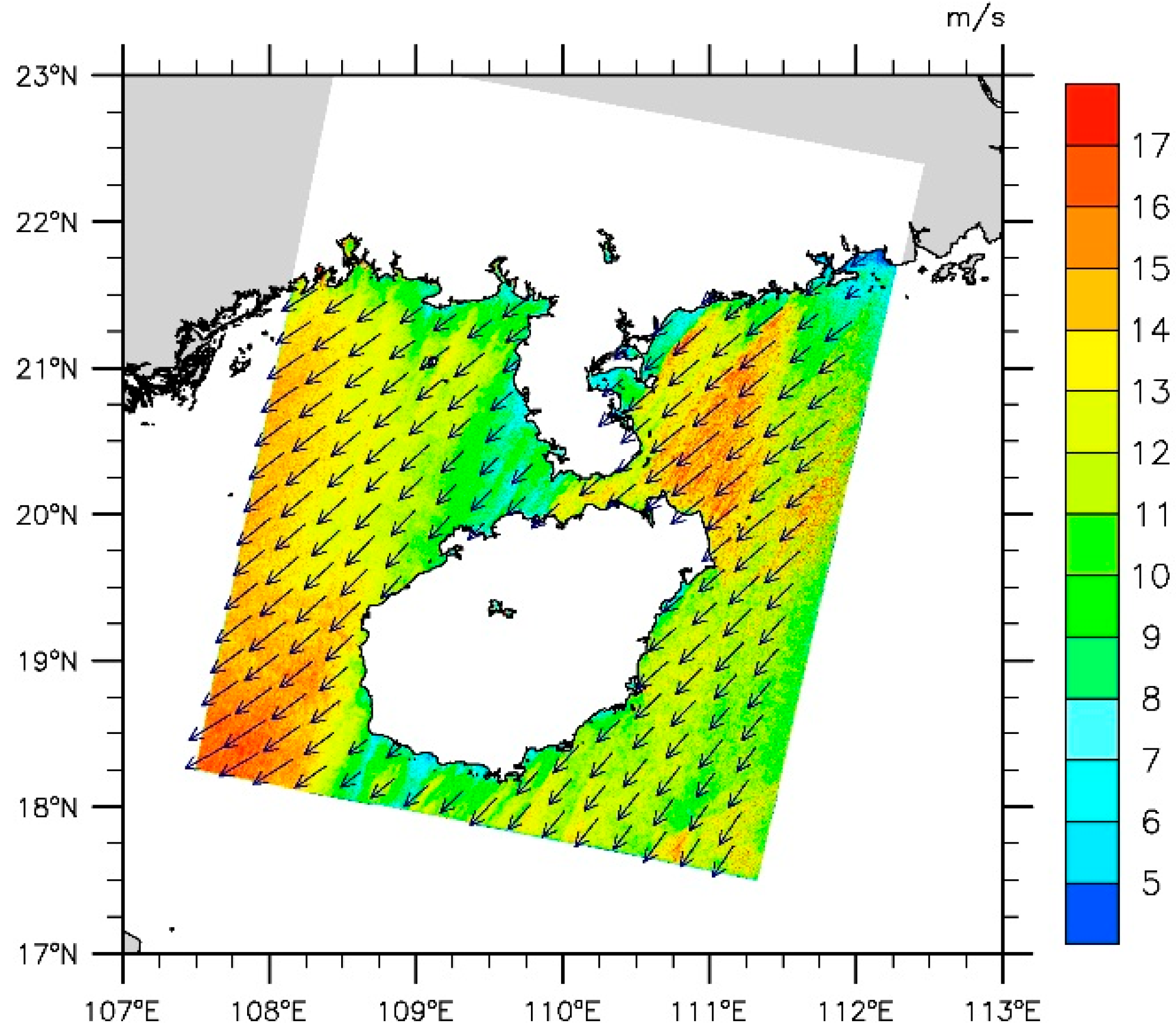
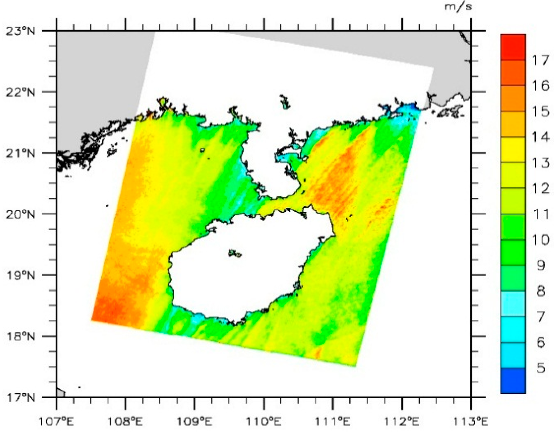
2.1. SAR Satellite Images and Wind Retrieval Method

The European ENVISAT satellite has acquired C-band ASAR images worldwide during the years 2002–2012. ENVISAT SAR scenes have previously been used for offshore wind resources assessment in Europe [9,15] and a similar approach is followed here for wind retrieval over the SCS.

The image archive at the ESA has been searched for ENVISAT scenes acquired in Wide Swath Mode with either vertical (C_VV) or horizontal (C_HH) polarization in transmit and receive. The spatial resolution of the WSM product is 150 m and the swath width is 400 km. The raw data is first calibrated to give the Normalized Radar Cross-section (NRCS), which expresses the radar return signal per unit area. NRCS depends on the instant wind stress over the sea surface and the radar viewing geometry.

Geophysical Model Functions (GMF) developed for scatterometer wind field retrievals can be used for retrieval of the instant wind speed from SAR observations of NRCS. The general form of these empirical GMFs is:

$$NRCS=U^{\gamma (\theta )}A(\theta )[1+B(\theta ,U)\cos \mathrm{\Phi }+C(\theta ,U)\cos 2\mathrm{\Phi }]$$

(1)

where ϴ is the local incidence angle; U is the wind speed at 10 m; ϕ is the wind direction with respect to the radar look direction; A, B, C and γ are the functions of incident angle and wind speed, and implicitly of the radar frequency. In this analysis, the GMF formulation called CMOD5.n is applied [16]. This GMF is tuned to observations of the Equivalent Neutral Wind (ENW) at 10 m in the open ocean i.e., effects of atmospheric stratification between the sea surface and 10 m are eliminated [17]. The output wind speed is thus given as ENW. The value of ENW is on average 0.2 m/s lower than the real wind speed in the tropics [18].

Equation (1) describes the backscatter-to-wind relationship for SAR observations acquired in C_VV whereas observations in C_HH need to be multiplied with a polarization ratio to compensate for their lower radar backscatter. Here, the polarization ratio of Mouche et al. [19] with directional dependence is used. In order to reduce the influence of long-period ocean waves and random image noise (speckle), NRCS needs to be spatially averaged before the wind retrieval. The original image pixels are averaged to the size 0.5 km in this study.

Wind speed retrieval from SAR requires a priori information about the wind direction as the SAR is only capable of observing each point at the sea surface from a single look angle. As a consequence, several wind speed and direction pairs correspond to a given value of NRCS. Our wind retrieval processing is initiated with wind direction inputs from the U.S. Navy Operational Global Atmospheric Prediction System (NOGAPS). The NOGAPS wind direction is from the lowest model layer, around 10 m above the surface. The model data has been interpolated from the original spatial resolution of 1° latitude and longitude to the 0.5-km grid of the satellite data. NOGAPS has a 6-h temporal resolution where the times nearest to the satellite data acquisitions are used.

An example of a wind speed map retrieved from SAR is shown in Figure 2 where the color coding shows the wind speed and the arrows give the input wind direction from NOGAPS. The winds are from the northeast, which is the prevailing wind direction in winter in the area. The image shows detailed wind speed variability around the island of Hainan with wind speed gradients near the coastlines especially on the sheltered sides of the land masses. The impact of the land topography is also noticeable.

Figure 2. Wind field retrieved from ENVISAT ASAR WSM data for 2 November 2009 at 02:36 UTC.

Figure 2. Wind field retrieved from ENVISAT ASAR WSM data for 2 November 2009 at 02:36 UTC.

The ENVISAT ASAR data set collected over the SCS amounts to 460 scenes in total (364 in C_VV and 96 in C_HH). Table 1 lists the number of scenes per year and per month. The scenes are almost equally distributed over the calendar year. A total of 379 scenes are morning passes acquired around 10:30 local time and 81 are evening passes acquired around 22:30 local time.

Table 1. SAR data used in the study per year and per month.

Year	Number of Scenes	Month	Number of Scenes
2003	1	January	35
2004	1	February	27
2005	12	March	39
2006	29	April	33
2007	62	May	36
2008	90	June	38
2009	58	July	53
2010	83	August	37
2011	100	September	34
2012	24	October	40
		November	53
		December	35

Table 1. SAR data used in the study per year and per month.

Year	Number of Scenes	Month	Number of Scenes
2003	1	January	35
2004	1	February	27
2005	12	March	39
2006	29	April	33
2007	62	May	36
2008	90	June	38
2009	58	July	53
2010	83	August	37
2011	100	September	34
2012	24	October	40
		November	53
		December	35

2.2. Scatterometer Wind Vectors

ASCAT Ocean Surface Wind Vectors data at 10 m height and 12.5 km resolution from 2009 to 2013 have been used in this study. The ASCAT data were processed by the National Oceanic and Atmospheric Administration (NOAA) utilizing measurements from ASCAT aboard the EUMETSAT METOP satellite at C-band. These scatterometer observations have similarities to C-band SAR; for example, the spectrum of capillary and short gravity waves is efficiently sensed by both sensor types, and a GMF can be used to calculate the wind speed. The major differences are that (1) wind direction can be calculated from scatterometers because they obtain multiple looks from different angles; (2) the spatial resolution is coarser than for a SAR instrument; (3) a mask is applied to scatterometer wind products eliminating winds over coastal seas; and (4) a scatterometer can provide one or two observations per day over most of the globe, whereas SAR sensing is more irregular [1].

The location of one of the ASCAT image frames is shown in Figure 3 where the color coding shows the wind speed and the black dots represent the locations of the satellite pixels. There are 5578 ASCAT scenes from March 2009 to July 2013 covering the South China Sea (see Table 2). Also, 2537 of the scenes are morning passes acquired around 09:00 local time and 3041 are evening passes acquired around 21:00 local time.

Figure 3. Wind field retrieved from ASCAT data for 2 March 2011 at 01:46 UTC.

Figure 3. Wind field retrieved from ASCAT data for 2 March 2011 at 01:46 UTC.

Table 2. ASCAT data used in the study per year.

Year	2009	2010	2011	2012	2013
Num of ASCAT scenes	1074	1282	1263	1297	662

Table 2. ASCAT data used in the study per year.

Year	2009	2010	2011	2012	2013
Num of ASCAT scenes	1074	1282	1263	1297	662

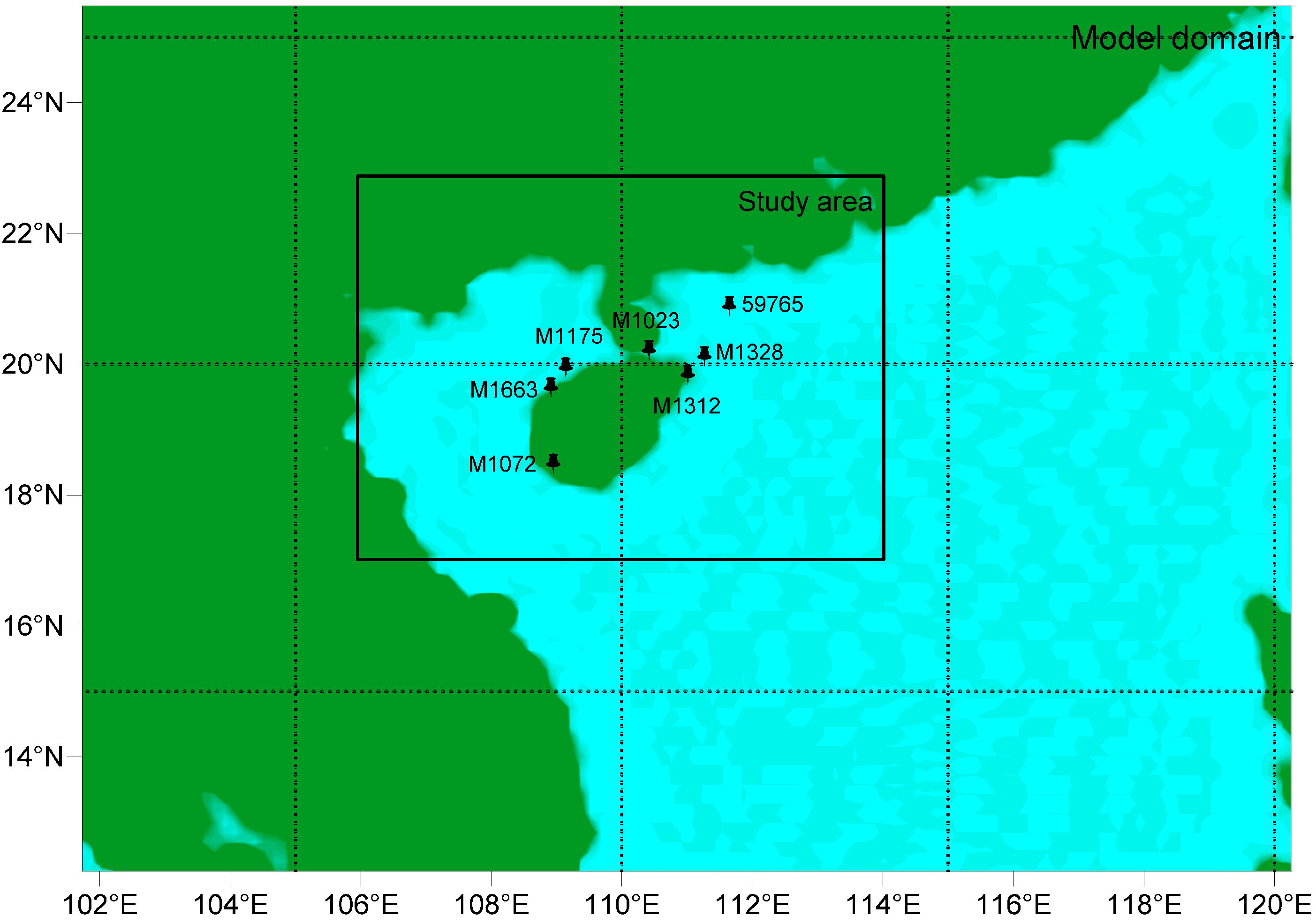
2.3. Wind Observations from Meteorological Stations

The meteorological observations over SCS is provided by Climate Center of Hainan Meteorological Bureau (see Figure 1 for specific locations), including hourly wind speed and wind direction observed at 10 m from seven in situ measurement stations. The data periods with the first and last observations from each of the seven met-masts used in the comparison study are listed in Table 3. The first four masts are located on islands in the ocean as close as 88 km, 31.5 km, 5.42 km and 2.2 km from the nearest continental coast, all are of relatively high data quality. The three masts from M1312 to M1663 are located on land at 0.05 km, 0.14 km and 0.48 km distance from the ocean. Observational environments of these masts are acceptable, large flat ground.

Table 3. In situ data from the seven masts are used in the comparison study. The altitude of met mast (H in m) and distance (D in km) to the nearest continental coast (−) or ocean (+) are given for all masts.

Met Mast	H	D	Observation Period
59765	0	−88	2010-07-23~2012-12-31
M1328	0	−31.5	2010-05-04~2012-12-31
M1072	0	−5.42	2010-04-27~2012-10-12
M1175	0	−2.2	2009-01-01~2012-10-12
M1312	0	0.05	2007-07-18~2012-10-12
M1023	3	0.14	2007-12-26~2012-10-12
M1663	8	0.48	2007-11-19~2012-10-12

Table 3. In situ data from the seven masts are used in the comparison study. The altitude of met mast (H in m) and distance (D in km) to the nearest continental coast (−) or ocean (+) are given for all masts.

Met Mast	H	D	Observation Period
59765	0	−88	2010-07-23~2012-12-31
M1328	0	−31.5	2010-05-04~2012-12-31
M1072	0	−5.42	2010-04-27~2012-10-12
M1175	0	−2.2	2009-01-01~2012-10-12
M1312	0	0.05	2007-07-18~2012-10-12
M1023	3	0.14	2007-12-26~2012-10-12
M1663	8	0.48	2007-11-19~2012-10-12

2.4. WRF Model Setup

The WRF model is a meso-scale numerical weather prediction system designed to serve both operational forecasting and atmospheric research needs [20]. In this study, we used version 3.4 of the Advanced Research WRF (ARW-WRF) model for one year (2011) of simulations at spatial resolution 15 km over the model domain (Figure 3).

Two main steps are used to combine the multiple satellite data and the pure WRF model output together: A relatively pure simulation based on the NCEP Climate Forecast System Reanalysis data, which from now on we will refer as “control”; and a simulation with the scatterometer data (here meaning ASCAT data) and SAR data assimilated into WRF model simulation files gotten from control runs, referred to here as “assimilation”.

2.4.1. Control Simulation

The model setup for the control simulation is described in Table 4. It is worth noting that the grid used covers the region of interest as shown in Figure 3. The choice of physical parameterizations is based upon the experiments done by Hahmann [20].

Table 4. Summary of model and system setup and physical parameterizations used in the control WRF simulations.

Model Setup:
WRF (ARW) Version 3.4 Model domain (121 × 92 grid points) with 15 km grid spacing on a Mercator projection (Figure 1). 36 vertical levels with model top at 50 hPa; eight of these levels are placed within 300 m of the surface.
Simulation Setup:
Initial, boundary conditions, and fields for grid nudging come from the NCEP Climate Forecast System Reanalysis data at 0.5° × 0.5° resolution [21]. Sea surface temperature (SST) and sea-ice fractions come from the dataset produced at USA NOAA/NCEP at 1/12° × 1/12° resolution [22] and are updated daily. Runs are started (cold start) at 00:00 UTC every 10 days and are integrated for 11 days, the first 24 h of each simulation are disregarded. Model output: Hourly. Time step in most simulations: 90 s. Grid nudging on model domain; nudging coefficient 0.0003 s−1 for wind, temperature and specific humidity.
Physical Parameterizations:
Precipitation: Thompson graupel scheme (option 8), Kain-Fritsch cumulus parameterization (option 1). Radiation: RRTM scheme for long-wave (option 1); Dudhia scheme for shortwave (option 1). PBL and land surface: Mellor-Yamada-Janjic scheme (option 2), Eta similarity (option 2) surface-layer scheme, and Noah Land Surface Model (option 2). Diffusion: Simple diffusion (option 1); 2D deformation (option 4); 6th order positive definite numerical diffusion (option 2); rates of 0.06; no vertical damping. Positive definite advection of moisture and scalars.

Table 4. Summary of model and system setup and physical parameterizations used in the control WRF simulations.

Model Setup:
WRF (ARW) Version 3.4 Model domain (121 × 92 grid points) with 15 km grid spacing on a Mercator projection (Figure 1). 36 vertical levels with model top at 50 hPa; eight of these levels are placed within 300 m of the surface.
Simulation Setup:
Initial, boundary conditions, and fields for grid nudging come from the NCEP Climate Forecast System Reanalysis data at 0.5° × 0.5° resolution [21]. Sea surface temperature (SST) and sea-ice fractions come from the dataset produced at USA NOAA/NCEP at 1/12° × 1/12° resolution [22] and are updated daily. Runs are started (cold start) at 00:00 UTC every 10 days and are integrated for 11 days, the first 24 h of each simulation are disregarded. Model output: Hourly. Time step in most simulations: 90 s. Grid nudging on model domain; nudging coefficient 0.0003 s−1 for wind, temperature and specific humidity.
Physical Parameterizations:
Precipitation: Thompson graupel scheme (option 8), Kain-Fritsch cumulus parameterization (option 1). Radiation: RRTM scheme for long-wave (option 1); Dudhia scheme for shortwave (option 1). PBL and land surface: Mellor-Yamada-Janjic scheme (option 2), Eta similarity (option 2) surface-layer scheme, and Noah Land Surface Model (option 2). Diffusion: Simple diffusion (option 1); 2D deformation (option 4); 6th order positive definite numerical diffusion (option 2); rates of 0.06; no vertical damping. Positive definite advection of moisture and scalars.

2.4.2. Assimilation

Data assimilation is the technique by which observations are combined with a numerical weather prediction product (the first guess) and their respective error statistics to provide an improved estimate (the analysis) of the atmospheric state. Variational (Var) data assimilation achieves this through the iterative minimization of a prescribed cost function as Equation (2) [23]:

$$J=\frac{1}{2}{(x-x_b)}^T{B}^{-l}(x-x_b)+\frac{1}{2}{[H(x)-y_{obs}]}^T{o}^{-l}[H(x)-y_{obs}]$$

(2)

where x is the gridded analysis; x_b is the first guess (or background); y_obs represents the observation; B and O are the background and observation error covariance matrices, respectively; H is the observation operator used to transform the gridded analysis x to observation space for comparison against observation y_obs. This solution represents a posteriori maximum likelihood (minimum variance) estimate of the true state of the atmosphere given the two sources of a priori data: the first guess (or background) x_b and observations y_obs [24].

In this paper, it is the three-dimensional variational (3D-Var) data assimilation system that we used to assimilate satellite data with the wrfout product. The choice of the parameters in the WRFDA system is listed as: Background error statistics from generic BE data (cv_ option = 3); the first guess from the control WRF runs; primary quality control and thinning, such as excluding the satellite data with low accuracy, thinning the SAR data into 15 km; observations processed by OBSPROC module which is built in WRFDA system; and observation error and the response of BE length scalling parameters from the default settings for this observation.

3. Spatial Averaging and Post-Processing Procedure

SAR winds were retrieved as spatial means whereas in situ measurements were temporal means obtained at one point. Here, SAR-retrieved wind fields were compared to measurements from the meteorological masts using a simple box averaging method and a post-processing procedure approach. The box averaging is done through processing of the original SAR wind maps with pixels sizes of 0.5 km (Figure 2) to maps with 5 km pixel size (Figure 4) at every scanning point. After spatial averaging, SAR wind speed at each pixel represents the mean wind of the all the pixels within a 5 km square box surrounding it. The SAR wind speed at the nearest pixel to the in situ site with a distance between them of usually less than 1 km is selected to compare against the in situ measurement.

Figure 4. Spatial averaging wind field retrieved from ENVISAT ASAR WSM data for 2 November 2009 at 02:36 UTC.

Figure 4. Spatial averaging wind field retrieved from ENVISAT ASAR WSM data for 2 November 2009 at 02:36 UTC.

The post-processing procedure is a must for quantitative data validation. Satellite data and in situ measurements can only be compared “qualitatively” without post-processing, especially in the coastal areas. As listed in Table 3, most of the observation sites we used in this area are located on the coastal area. The observation environments in these in situ observational stations are strictly according to the China Ground-based Observation Criterion. The roughness length for the observational environments of the in situ stations is set to 0.02 m in this study. The topography and roughness over the satellite scanning area are often very different from those over the in situ stations. Based on the concept and technique described by Larsén [25], we transform the wind between different topographies and surface roughness, keeping the wind variability consistent through the physical description, to the in situ site condition.

Briefly, to introduce the generalization process, we first calculate the friction velocity (u_*) and the roughness length (Z₀) obtained from the satellite wind maps through a combination of Equation (3) with Equation (4):

$$u_{10}=\frac{u_{*}}{k}[\ln \frac{10}{z_0}]$$

(3)

where u₁₀ is the equivalent neutral wind speed at 10 m retrieved from the satellite, k is the von Kármán constant (0.4) and Z₀ is the roughness length, which can be described as:

$$z_0={\alpha }_c\frac{u_{*}^2}{g}$$

(4)

where α_c is Charnock’s parameter (here set to 0.0144) and g is the gravitational acceleration of the Earth.

Then, the geostrophic wind, G, is calculated from u_* and Z₀ through the geostrophic drag law [26]:

$$G=\frac{u_{*}}{k}\sqrt{{(\ln \frac{u_{*}}{f{z}_0}-A)}^2+B^2}$$

(5)

where f is the Coriolis parameter and A = 1.8 and B = 4.5 are dimensionless parameters according to [27]. Neutral atmospheric conditions are assumed as no temperature observations are available for estimation of the atmospheric stability. The fundamental principle of this process is that G remains the same before and after the generalization. Under the same G but with a new roughness length for the meteorological masts site condition, here Z₀ = 0.02 m, a new friction velocity, u_*, is obtained through Equation (5). Using this new set of u_* and Z₀ and Equation (3), we obtain the processed satellite wind speed, which will be validated by the in situ measurements.

In order for the statistics from the hourly in situ measurements to match well with the averaging technique, a 70 min average centered at the satellite recording time is used, which means the in situ measurements at the two sides of satellite recording time are averaged. After calculating and selecting, seven collocated data series of wind speed from satellite data and in situ measurement in SCS region are ready to be compared.

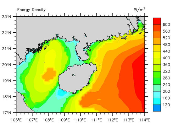
4. Wind Resource Statistics

The Weibull probability distribution function is commonly used to describe wind speed data, as in the European Wind Atlas [2]. The available wind power density, E, may be calculated from the two Weibull parameters, the scale parameter A and the shape parameter k, using the gamma function Γ, and the air density ρ as

$$E=0.5\times \rho \times A^3\times \mathrm{\Gamma }(1+\frac{3}{k})$$

(6)

Previous studies have shown that a total of 60–70 randomly selected and perfectly accurate samples (i.e., SAR scenes) are required to characterize the mean wind speed and Weibull scale parameter with an accuracy of 10% for sites with a limited diurnal wind variability [28]. In the SCS, the diurnal wind patterns could have a significant impact on the wind resource which cannot be resolved by satellite SAR.

5. Validation Results

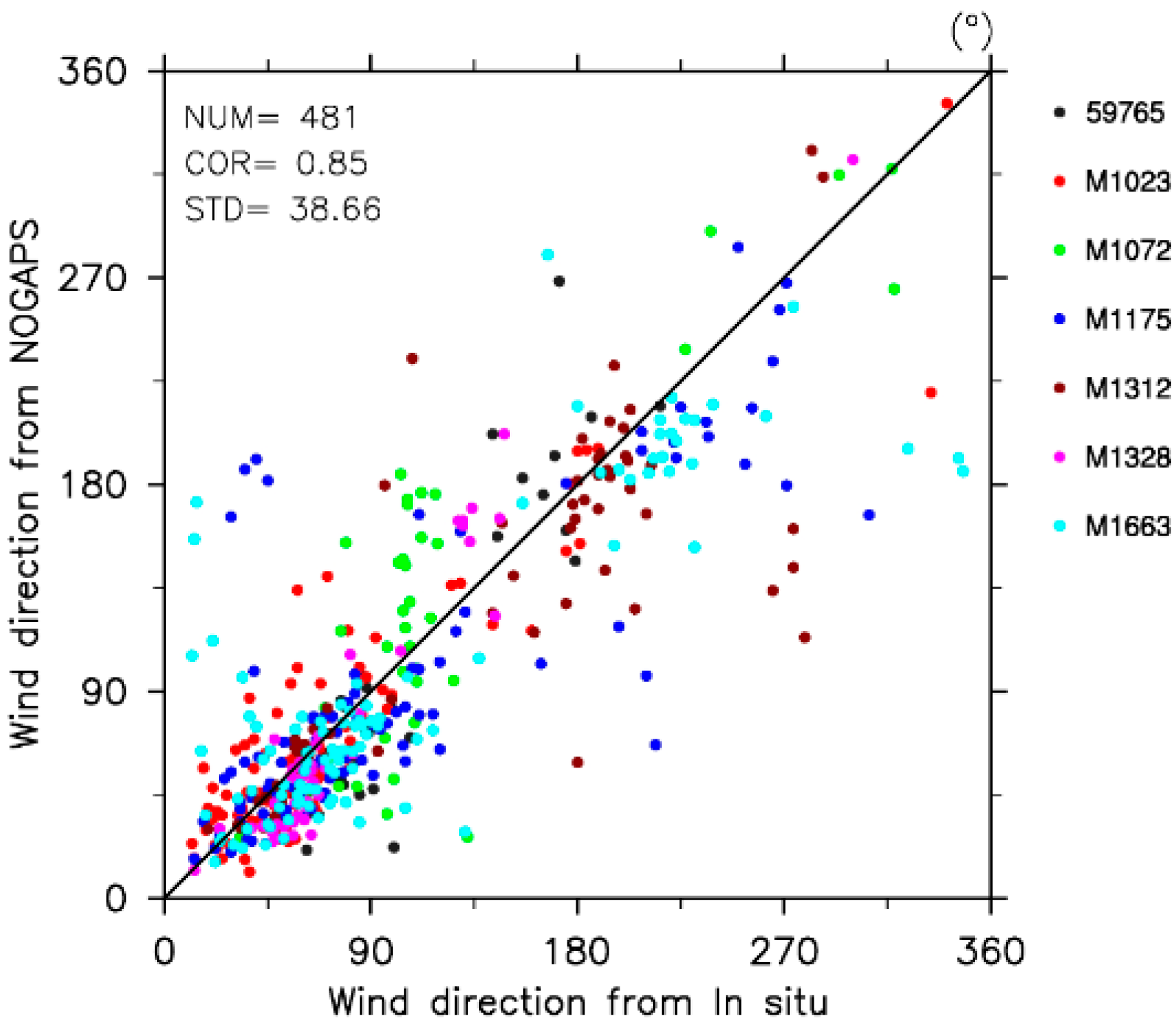
5.1. Wind Direction between In Situ Data vs. SAR

The wind direction in SAR images are from the NOGAPS wind directions interpolated in time and space to match the SAR data. The wind directions from all masts versus NOGAPS are shown in Figure 5, and a few observations near 0° and 360° are removed. The statistical results show a standard deviation (SD) of 38.66° and correlation coefficient of R 0.85. The wind roses of every mast are then investigated (not shown here), and it is shown that the features from NOGAPS are similar to these from in situ measurements, indicating a satisfactory consistency in wind direction at most of the in situ sites except for M1072, partly because of the small statistical number in this site (less than 45). This wind direction uncertainty affects the accuracy of the SAR wind speed retrieval.

Figure 5. Wind directions from in situ measurements vs. NOGAPS.

Figure 5. Wind directions from in situ measurements vs. NOGAPS.

5.2. Wind Speed between In Situ Data vs. SAR

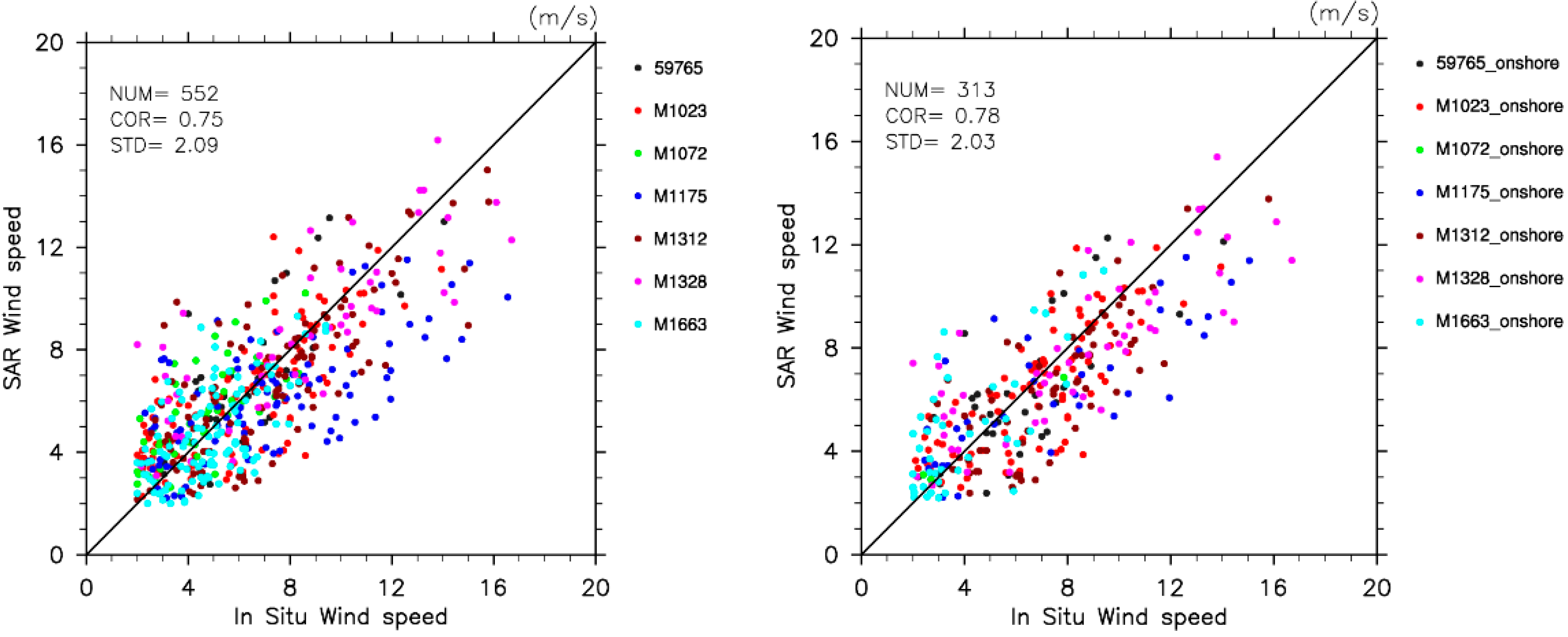
The comparison results on wind speed are calculated for each meteorological station. The overall data are included in the plot between in situ wind speed and SAR-based wind speed shown in Figure 6 (left) and winds less than 2.0 m/s are excluded. Table 5 shows the results of the correlation analyses between them. The correlation coefficients are smaller than 0.8 and standard deviations are larger than 1.8 m/s at most of the meteorological masts. In all, it shows that regression using N = 552 samples of collocated wind speed observed at meteorological stations and SAR-based wind speed results in R = 0.75, SD = 2.09 m/s. The overall mean error in Table 5 is −0.27 m/s, which represents that the SAR winds underestimate the in situ wind speeds a little bit. For the onshore samples (Figure 6 (right)), which means the wind flows from ocean to land, the statistical results show a correlation coefficient of R = 0.78, with a standard deviation of 2.03 m/s, indicating the higher retrieval accuracy of SAR data over the ocean. This phenomenon can be explained in this way: The retrieval of SAR wind is based on the interaction between the sea surface winds and ocean waves, and it can reflect the ocean winds very well. When the wind flows from land to ocean, it holds lots of effects of the land surface, which can impose a negative effect on the comparison results.

Figure 6. In situ wind speeds from seven meteorological stations vs. SAR wind speeds for all samples (left, N = 552) and onshore samples (right, N = 313).

Figure 6. In situ wind speeds from seven meteorological stations vs. SAR wind speeds for all samples (left, N = 552) and onshore samples (right, N = 313).

Table 5. Statistic results for wind speed between in situ data vs. SAR-wind. N is the number of comparing samples, R is the correlation coefficient, SD is the standard deviation (m/s); ME is the mean error (m/s).

Station No.	N	R	SD (m/s)	ME (m/s)
59765	31	0.74	2.00	0.67
M1328	50	0.81	2.37	−0.01
M1072	52	0.72	1.41	0.84
M1175	99	0.67	2.5	−0.46
M1312	108	0.77	2.09	−1.34
M1023	106	0.74	1.86	−0.07
M1663	106	0.62	1.55	−0.20
All	552	0.75	2.09	−0.27

Table 5. Statistic results for wind speed between in situ data vs. SAR-wind. N is the number of comparing samples, R is the correlation coefficient, SD is the standard deviation (m/s); ME is the mean error (m/s).

Station No.	N	R	SD (m/s)	ME (m/s)
59765	31	0.74	2.00	0.67
M1328	50	0.81	2.37	−0.01
M1072	52	0.72	1.41	0.84
M1175	99	0.67	2.5	−0.46
M1312	108	0.77	2.09	−1.34
M1023	106	0.74	1.86	−0.07
M1663	106	0.62	1.55	−0.20
All	552	0.75	2.09	−0.27

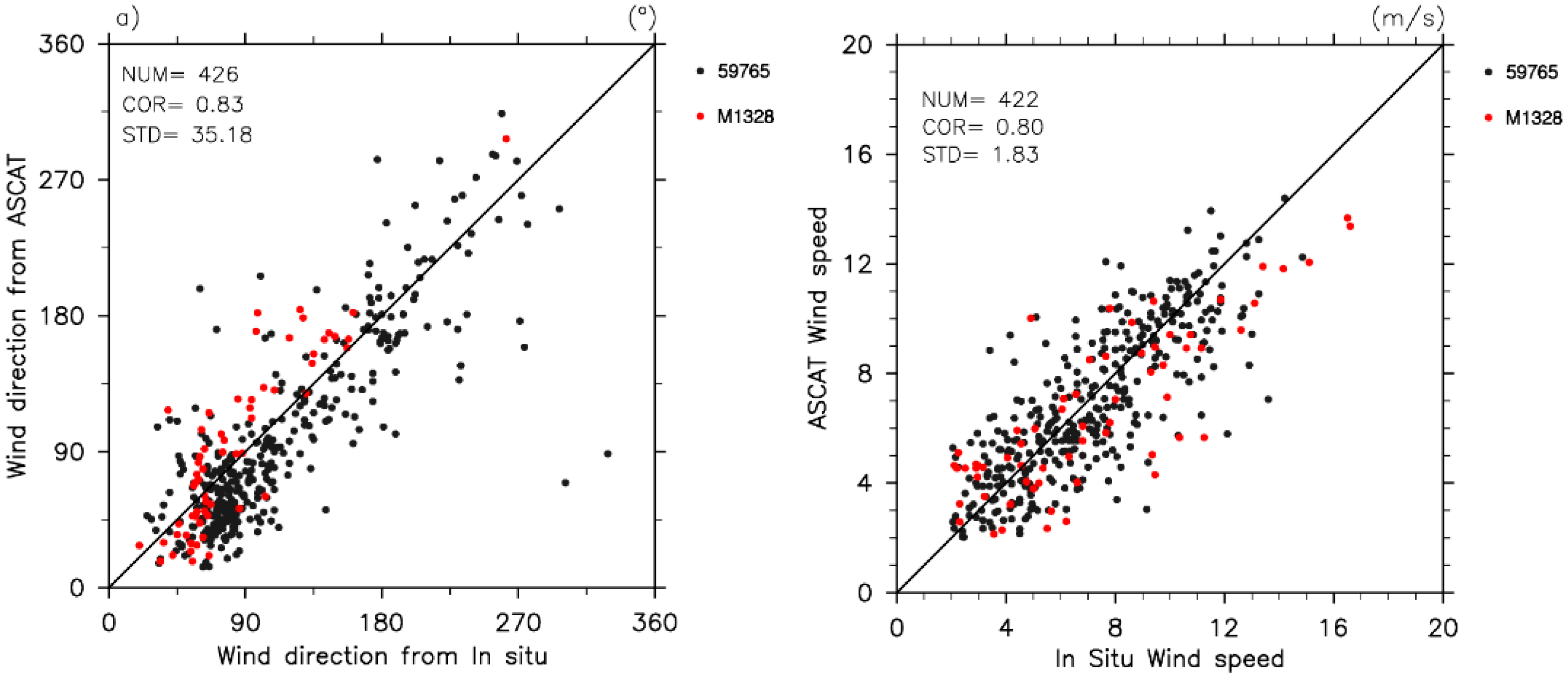
5.3. Wind between Scatterometer Data and In Situ Data

We have also validated the accurancy of ASCAT wind vectors using the in situ measurements in the SCS area. Similar to the method used in SAR data, the scatterometer wind at the nearest pixel to the in situ site has been selected to compare against the in situ measurements, and the post-processing procedure described in Section 3 has been applied to overcome the adverse effect of the different topographies and surface roughness between the comparative candidates. The spatial resolution of the ASCAT is 12.5 × 12.5 km and there is a long distance from location of the effective retrieval winds to the coastline as shown in Figure 3. Therefore, when we selected the nearest ASCAT wind data for the seven in situ stations at 30 km around, only two stations are qualified to be used to validate the ASCAT data.

The comparison results on wind direction and wind speed are presented in Figure 7. In the left figure, a few observations near 0° and 360° are removed, and in the right figure, observations less than 2 m/s are removed. The good consistency between in situ data and scatterometer data in the wind directions (Figure 7 (left)) leads to the high correlation coefficient and relatively low standard deviation (Figure 7 (right) and Table 6) in the wind speeds. The statistic results can be compared with the SAR data validation results at 59765 and M1328 (Table 5). For M1328, SAR and ASCAT have similar N, similar R and similar SD, and only mean error is different, indicating a satisfactory level of accuracy which was similar for SAR and scatterometer winds in the study area. It is important to note that the satellites provide the equivalent neutral wind (ENW) whereas the masts give the real wind. This might explain some of the deviation between satellite and in situ winds shown here.

Table 6. The same as Table 5, but for ASCAT.

Station No.	N	R	SD (m/s)	ME (m/s)
59765	358	0.79	1.77	−0.32
M1328	64	0.82	2.13	−0.85
All	422	0.80	1.83	−0.40

Table 6. The same as Table 5, but for ASCAT.

Station No.	N	R	SD (m/s)	ME (m/s)
59765	358	0.79	1.77	−0.32
M1328	64	0.82	2.13	−0.85
All	422	0.80	1.83	−0.40

Figure 7. In situ wind directions (left) and wind speeds (right) vs. ASCAT wind.

Figure 7. In situ wind directions (left) and wind speeds (right) vs. ASCAT wind.

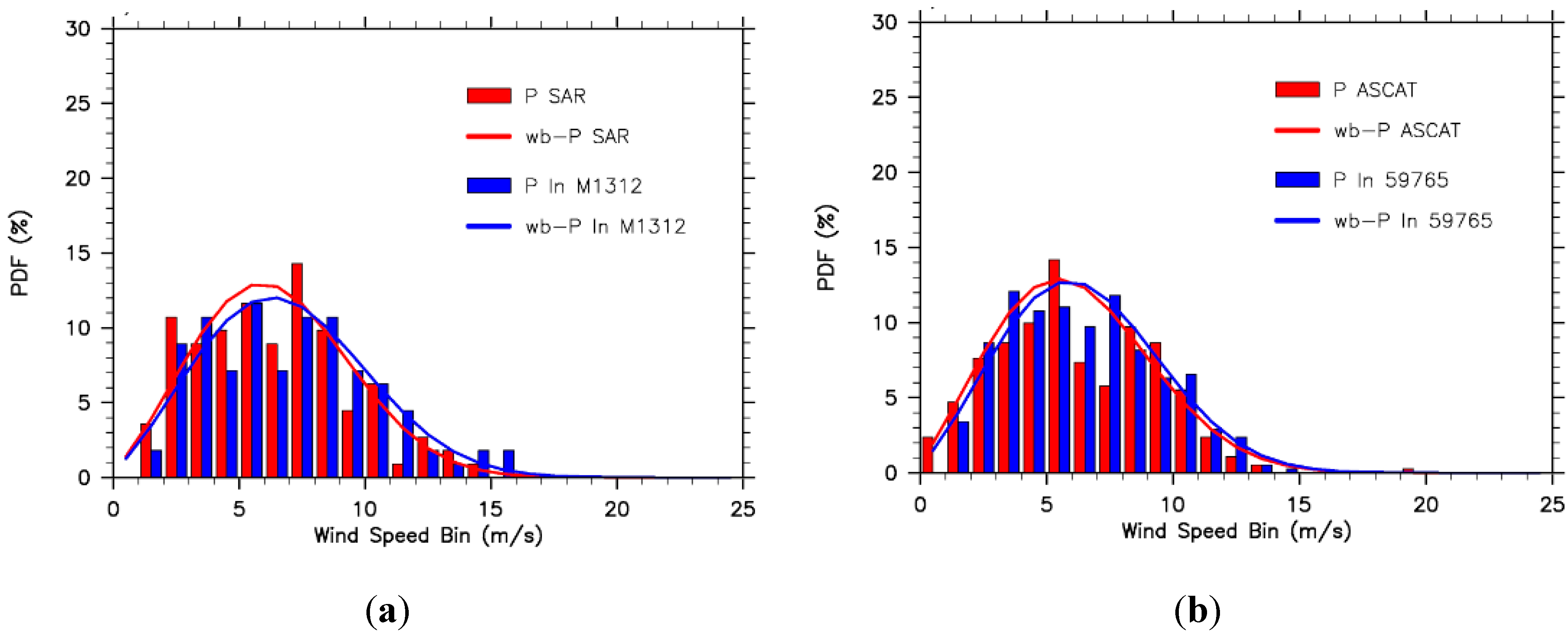
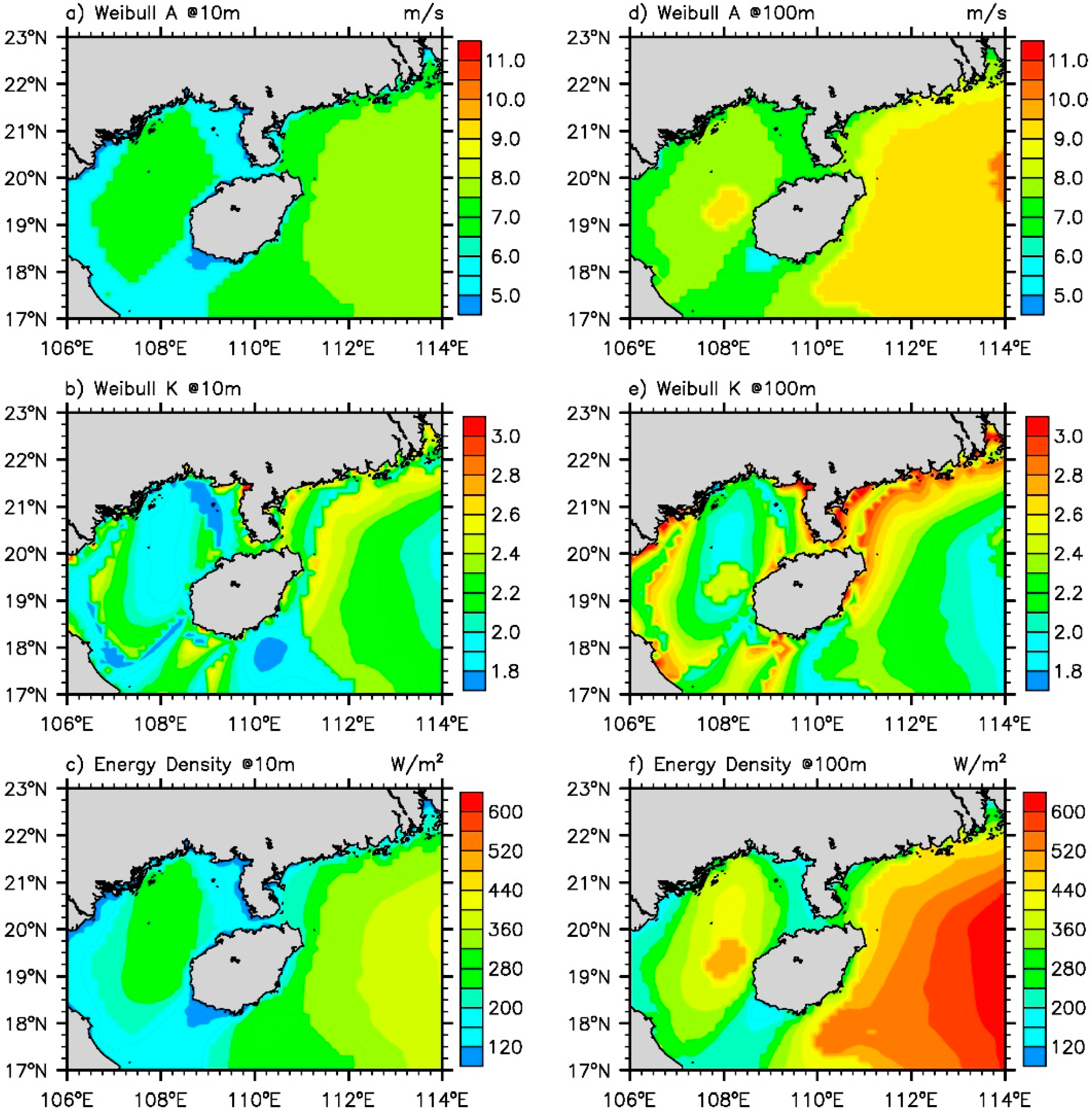
5.4. Weibull Parameter Based on Satellite Data

Due to the different periods of operation, the number of co-located mast and satellite samples is limited. As noted in Section 4, the perfectly accurate samples for characterizing the Weibull parameters (Equation (6)) should not be less than 60–70. Because the samples at 59765 and M1328 for SAR-based wind speed are all less than 60, it is difficult to compare SAR and ASCAT for the same station in this part. Therefore, the SAR-based and ASCAT-based wind speed distributions are calculated at M1312 and 59765, respectively. The statistical results show that the Weibull scale parameter of A and the shape parameter of K computed at M1312 are 10.4 m/s and 2.49 for the 108 samples. These two Weibull parameters are first determined from SAR, yielding a good agreement on the Weibull fitting lines with the in situ measurements (Figure 8a). A similar agreement on the wind resource statistics are found between the ASCAT data and in situ data at 59765 (Figure 8b). This high consistency makes the multiple satellite data fusion possible.

Figure 8. Histograms of in situ winds (red bars) and satellite retrieval winds (blue bars) as well as their Weibull fits (red curves for in situ winds and blue curves for satellite retrieval winds): (a) in situ winds and the co-located SAR winds at M1312; (b) in situ winds and the co-located ASCAT winds at 59765.

Figure 8. Histograms of in situ winds (red bars) and satellite retrieval winds (blue bars) as well as their Weibull fits (red curves for in situ winds and blue curves for satellite retrieval winds): (a) in situ winds and the co-located SAR winds at M1312; (b) in situ winds and the co-located ASCAT winds at 59765.

6. Satellite Data Assimilation

It has been shown that the satellite retrieval winds over the ocean agree well with the in situ measurements. Meanwhile, these quasi-observation data, ASCAT- and SAR-based retrieval winds hold a low time resolution and can only characterize the 10 m wind over the ocean, which make them missing a lot of wind events. Conversely, the WRF data sets give the whole year simulations with hourly outputs in multiple vertical levels, while the pure simulations from WRF usually deviate from the in situ measurements [29].

To make full use of the multiple source data in the offshore wind resources assessment, the WRFDA data assimilation system is used to combine the wind speed information from satellite scenes with the simulation information from WRF. In this study, WRF model experiments are carried out for control runs and assimilation runs during 2011. Since the spatial resolution of SAR wind maps is about 0.5 km, which is much higher than the spatial resolution of WRF model used here, these data are resampled to 15 km before they get into the assimilation system. As noted in Section 5, the retrieval credibility of the satellite data near the coastal lines is lower than the open ocean, so the retrieval wind speeds near the coastal lines are removed in the assimilation experiments, also.

The control simulation covers the period from 1 January 2011 to 31 December 2011, with hourly outputs. Before the assimilation experiments, ASCAT retrieval winds at ten points and SAR winds at five points scattered over the study area were extracted randomly from the satellite datasets. Then, ASCAT retrieval winds and SAR retrieval winds from the rest pixels are assimilated into the WRF model. Of all the 8760 h in 2011, there are 743 h corresponding with ASCAT scanning time and 75 h with SAR scanning time. Based on the WRFDA data assimilation system, these satellite data were assimilated at the corresponding hours, generating the hourly assimilation results of the total 818 samples.

Table 7 summarizes the number of co-located samples, correlation coefficient and root mean square error (RMSE) for the excluded ten points of ASCAT data which are scattered over the ocean at the study area. At these points, there are obvious improvement of correlation coefficient and RMSE. Similar test experiments are processed by SAR retrieval winds at five excluded points, and also show the similar results (not shown). Meanwhile, the high correlation coefficients and low RMSEs in Table 7 illustrate the good overall agreements on the WRF simulated winds and satellite retrieval winds, especially for the assimilated winds.

Table 7. Correlation coefficients and RMSE (m/s) calculated from control run and assimilation run with the ASCAT retrieval winds at ten points, respectively. N is the number of satellite samples at the location during 2011.

Station Location	N	Statistical Variables	Control Run	Assimilation Run
(115.5°E, 20.5°N)	242	correlation coefficient	0.85	0.96
		RMSE (m/s)	1.94	0.93
(108.5°E, 18.7°N)	270	correlation coefficient	0.86	0.91
		RMSE	1.91	1.57
(111.8°E, 19.5°N)	226	correlation coefficient	0.92	0.96
		RMSE (m/s)	1.36	0.97
(108.0°E, 20.0°N)	300	correlation coefficient	0.89	0.96
		RMSE (m/s)	1.50	1.00
(108.0°E, 17.5°N)	290	correlation coefficient	0.80	0.90
		RMSE (m/s)	1.89	1.29
(112.0°E, 18.5°N)	250	correlation coefficient	0.92	0.95
		RMSE (m/s)	1.39	1.05
(108.0°E, 20.0°N)	299	correlation coefficient	0.89	0.96
		RMSE (m/s)	1.87	1.10
(107.0°E, 19.0°N)	300	correlation coefficient	0.85	0.95
		RMSE (m/s)	1.93	1.02
(103.0°E, 19.0°N)	237	correlation coefficient	0.91	0.96
		RMSE (m/s)	1.54	1.02
(109.0°E, 20.2°N)	290	correlation coefficient	0.86	0.92
		RMSE (m/s)	1.86	1.35

Table 7. Correlation coefficients and RMSE (m/s) calculated from control run and assimilation run with the ASCAT retrieval winds at ten points, respectively. N is the number of satellite samples at the location during 2011.

Station Location	N	Statistical Variables	Control Run	Assimilation Run
(115.5°E, 20.5°N)	242	correlation coefficient	0.85	0.96
		RMSE (m/s)	1.94	0.93
(108.5°E, 18.7°N)	270	correlation coefficient	0.86	0.91
		RMSE	1.91	1.57
(111.8°E, 19.5°N)	226	correlation coefficient	0.92	0.96
		RMSE (m/s)	1.36	0.97
(108.0°E, 20.0°N)	300	correlation coefficient	0.89	0.96
		RMSE (m/s)	1.50	1.00
(108.0°E, 17.5°N)	290	correlation coefficient	0.80	0.90
		RMSE (m/s)	1.89	1.29
(112.0°E, 18.5°N)	250	correlation coefficient	0.92	0.95
		RMSE (m/s)	1.39	1.05
(108.0°E, 20.0°N)	299	correlation coefficient	0.89	0.96
		RMSE (m/s)	1.87	1.10
(107.0°E, 19.0°N)	300	correlation coefficient	0.85	0.95
		RMSE (m/s)	1.93	1.02
(103.0°E, 19.0°N)	237	correlation coefficient	0.91	0.96
		RMSE (m/s)	1.54	1.02
(109.0°E, 20.2°N)	290	correlation coefficient	0.86	0.92
		RMSE (m/s)	1.86	1.35

Table 8. Validation of the control run and assimilation run with in situ measurements. N_S and N_A are the co-located samples for SAR and ASCAT, RMSE _ct (m/s) and RMSE_da (m/s) are the root mean square error for control runs and assimilation runs during 2011, ΔRMSE (m/s) is the difference between RMSE_da and RMSE_ct.

Station No.	Validation Results of SAR Wind Assimilation				Validation Results of ASCAT Wind Assimilation
	NS	RMSEct (m/s)	RMSEda (m/s)	ΔRMSE (m/s)	NA	RMSEct (m/s)	RMSEda (m/s)	ΔRMSE (m/s)
59765	48	8.58	5.71	−2.87	410	5.91	3.95	−1.96
M1328	33	7.08	7.81	0.73	369	7.34	6.62	−0.72
M1072	57	7.37	5.94	−1.43	521	6.69	5.63	−1.06
M1175	42	6.62	8.11	1.49	588	5.61	6.04	0.43
M1312	58	7.10	5.10	−2	598	4.30	4.59	0.29
M1023	47	5.53	5.17	−0.36	368	4.45	4.87	0.42
M1663	77	6.44	4.65	−1.79	539	7.34	6.07	−1.27

Table 8. Validation of the control run and assimilation run with in situ measurements. N_S and N_A are the co-located samples for SAR and ASCAT, RMSE _ct (m/s) and RMSE_da (m/s) are the root mean square error for control runs and assimilation runs during 2011, ΔRMSE (m/s) is the difference between RMSE_da and RMSE_ct.

Station No.	Validation Results of SAR Wind Assimilation				Validation Results of ASCAT Wind Assimilation
	NS	RMSEct (m/s)	RMSEda (m/s)	ΔRMSE (m/s)	NA	RMSEct (m/s)	RMSEda (m/s)	ΔRMSE (m/s)
59765	48	8.58	5.71	−2.87	410	5.91	3.95	−1.96
M1328	33	7.08	7.81	0.73	369	7.34	6.62	−0.72
M1072	57	7.37	5.94	−1.43	521	6.69	5.63	−1.06
M1175	42	6.62	8.11	1.49	588	5.61	6.04	0.43
M1312	58	7.10	5.10	−2	598	4.30	4.59	0.29
M1023	47	5.53	5.17	−0.36	368	4.45	4.87	0.42
M1663	77	6.44	4.65	−1.79	539	7.34	6.07	−1.27

In order to validate the assimilation results, it is necessary to use the independent in situ measurements on ships, lighthouses or buoys over the open ocean. Because of the lack of these measurements in this study, the seven offshore in situ measurements (see Section 2.3) are used in this part. The validation results are listed in Table 8. It shows an obvious improvement of RMSE at most stations (five out of seven) and a small increasing RMSE at M1328 for SAR wind assimilation experiments. Meanwhile, four out of seven stations is characteristic by the obvious improvement of RMSE for ASCAT wind assimilation experiments and the small increasing RMSE found in the other three stations are partly because of the large mask of the scatterometer wind products over coastal seas as shown in Figure 3 which introduced less wind information over the coastal area than SAR wind retrieval. On the other hand, the weak simulation capability of WRF near the coast and islands gives rise to the large deviation in Table 8, which also illustrate that it is a really good idea to assimilate satellite data and even in situ measurements in the future. Overall, the main point shown in Table 8 is that the results improve quite clearly when the satellite data are assimilated.

Figure 9 shows the maps of the 10 m and 100 m mean wind speed from WRF control run data and WRF assimilation run data. The patterns of the wind speeds from the assimilation runs both at 10 m and 100 m are similar to the control runs, but the wind speeds from the assimilation data are lower than those from the control run, mainly because the wind speeds from the control run are higher than those from the satellite data.

Figure 9. Maps of the mean wind speed at 10 m and 100 m from control run and assimilation run averaged with co-located samples: (a) wind speed at 10 m from control run, (b) wind speed at 10 m from assimilation run; (c) wind speed at 100 m from control run and (d) wind speed at 100 m from assimilation run.

Figure 9. Maps of the mean wind speed at 10 m and 100 m from control run and assimilation run averaged with co-located samples: (a) wind speed at 10 m from control run, (b) wind speed at 10 m from assimilation run; (c) wind speed at 100 m from control run and (d) wind speed at 100 m from assimilation run.

The 818 pairs of numerical winds from the control simulation and from the assimilation run are then linked and established a statistical relationship. Based on this relationship, the numerical winds at other hours are modified. Finally, a whole-year hourly reconstructed wind data fully combining the information from multiple satellites as well as the numerical model (WRF) is achieved.

The wind energy resource statistics in the SCS are calculated based on the hourly reconstructed wind data using the method in Section 4. The resulting maps are presented in Figure 10, showing the Weibull A and k, and wind power density E, at 10 m and 100 m height. The spatial variability of the wind energy resources at these two heights is similar, but the absolute values are higher at 100 m than at 10 m. At 100 m height (Figure 10 (right)), Weibull A ranges from 7.5 m/s along the eastern Hainan coast to 9.5 m/s over the eastern part of the study area and from 7.5 m/s along the southwestern Hainan coast to 9.5 m/s over the western water area of this coast. Weibull k ranges from 1.9 over the open ocean, western and eastern parts of the study area, up to 2.5 near the coastlines. Wind power density values range from 400 to 600 W/m². The higher wind power density values are found over the southwestern and eastern parts of the study area.

Figure 10. Wind resource statistics based on 8760 reconstructed winds at 10 m (left) and 100 m (right) covering SCS. Panels top: (a) Weibull A (m/s); (b) Weibull k; (c) wind power density (W/m²), (d) Weibull A (m/s); (e) Weibull k; and (f) wind power density (W/m²).

Figure 10. Wind resource statistics based on 8760 reconstructed winds at 10 m (left) and 100 m (right) covering SCS. Panels top: (a) Weibull A (m/s); (b) Weibull k; (c) wind power density (W/m²), (d) Weibull A (m/s); (e) Weibull k; and (f) wind power density (W/m²).

7. Discussions

The aim of this paper is to study the application methods of multi-source satellite data in the Chinese offshore wind resources assessment, including the validation of the satellite data and satellite data assimilation technique. The validation accuracy depends, to a large degree, on the quality of the in situ measurements and the locations of the in situ site and the corresponding satellite pixel. All but one of the meteorological masts is on land. Human activities from residents living in the islands may affect the observational environment of the meteorological masts. The different topographies, surface roughness and the significant coastal wind gradients impose negative effects on the validation works. Further, it has not been possible to account for atmospheric stability effects on the mast observations due to a lack of temperature gradient observations.

Satellite winds retrieval and the post-processing procedure are all carried out based on the equivalent neutral atmospheric situation, whereas the real conditions over the SCS area are very unstable because of the very high sea surface temperature over this region (i.e., above 23 °C throughout the year). Therefore, we cannot expect a perfect agreement between the satellite and mast winds. Hypothetically, the lack of stability correction for the mast observations should reduce wind speed values at 10 m during unstable compared to neutral conditions, assuming a constant wind stress at the sea surface. This would result in a positive bias on the satellite ENW. The negative biases found in this study for both the SAR and scatterometer winds are most likely related to the limited fetch of the investigated stations or systematic biases in the wind retrieval algorithms.

Although the unstable conditions and the limited fetch in the study area add uncertainty to the SAR wind retrievals, the validation results show a higher consistency with in situ measurements than the validation results in Hangzhou Bay, China [30]. The deviations between satellite and in situ measurements found in this paper is higher than results from some European wind farm sites with near-neutral atmospheric conditions and real offshore masts [9].

In this paper, the satellite data are assimilated into WRF model by three-dimensional (3D-Var) data assimilation system. Although the choice of the parameters in the WRFDA system is preliminary or simple, and most choices are just according to the default settings, we established a feasible and applicable method that can be used to operate the offshore wind resources assessment in China. This method could be improved through lots of sensitivity experiments, such as more proper background error, len scaling and other relative assimilation parameters. An improvement of the accuracy of the satellite winds used for the assimilation is also desirable before the full benefit of the data assimilation can be achieved.

The robust validation of the reconstructed wind resource statistics is not done in this study, mainly because of the lack of in situ measurements on ships, lighthouses or buoys at the study area. The validation of the assimilation effects by the winds from the satellite pixels and the coastal measurements (Table 7 and Table 8) give us confidence that the final findings in this study are rational and credible to some extent. As for the weak simulation capability of WRF near the coast and islands, it would be interesting to assimilate the in situ measurements in the future.

8. Conclusions

The study outlines a methodology for combining multiple satellite winds and winds from WRF simulations in order to acquire the accurate reconstructed offshore winds which can be used for offshore wind resource assessment. In order to validate the satellite winds quantitatively, especially in the coastal areas, the study firstly converts the satellite winds into the processed satellite wind speed by post-processing procedure as introduced in Section 3. Then, the co-located satellite winds are validated by the in situ winds from seven meteorological sites on the coastal land of Hainan island. The standard deviation (SD) and correlation coefficient (R) between in situ wind speed and SAR-based (ASCAT-based) wind speed is 2.09 m/s (1.83 m/s) and 0.75 (0.80). When the offshore winds are excluded, the validated results at wind speeds show a significant improvement in SD and R, indicating that the satellite data are much more credible over the open ocean.

To make full use of these quasi-observed satellite data and hourly winds from WRF simulations, WRFDA data assimilation system has been used. Wind resource statistics based on the final reconstructed wind data illustrate that the wind power density at 100 m height ranges from 400 to 600 W/m² over the study area. These findings presented here as well as the methodology for combining the satellite winds and winds from WRF simulations are valuable in offshore wind resource assessment in China, where the in situ measurements on ships, lighthouses or buoys are very rare at this time.

References

1. Hasager, C.B.; Barthelmie, R.J.; Christiansen, M.B. Quantifying offhsore wind resources from satellite wind maps: Study area the North Sea. Wind Energy 2006, 9, 63–74. [Google Scholar] [CrossRef]
2. Troen, I.; Petersen, E.L. European Wind Atlas. Available online: https://www.etde.org/etdeweb/details_open.jsp?osti_id=5920204 (accessed on 23 August 2014).
3. Christiansen, M.B.; Koch, K.; Horstmann, J.; Hasager, C.B.; Nielsen, M. Wind resource assessment from C-band SAR. Remote Sens. Environ. 2006, 105, 68–81. [Google Scholar] [CrossRef]
4. Dagestad, K.F.; Horstmann, J.; Mouche, A.; Perrie, W.; Shen, H.; Zhang, B.; Li, X.; Monaldo, F.; Pichel, W.; Lehner, S.; et al. Wind Retrieval from Synthetic Aperture Radar—An Overview. Available online: http://orbit.dtu.dk/ws/files/59267621/SeaSAR2012_whitepaper_wind.pdf (accessed on 23 August 2014).
5. Xu, J.W.; Yong, L.; Zhang, X.Z.; Zhu, R. China offshore wind energy resources assessment with the QuickSCAT data. In Proceedings of the SPIE Remote Sensing of the Ocean, Sea Ice and Large Water Regions, Cardiff, UK, 13–15 September 2008.
6. Chou, K.-H.; Wu, C.-C.; Lin, S.-Z. Assessment of the ASCAT wind error characteristics by global dropwindsonde observations. J. Geophys. Res. 2013, 118, 9011–9021. [Google Scholar]
7. Johannessen, J.A. Coastal Observing Systems: The Role of Synthetic Aperture Radar. Available online: http://www.jhuapl.edu/techdigest/TD/td2101/johann.pdf (accessed on 23 August 2014).
8. Hasager, C.B.; Nielsen, M.; Astrup, P. Offshore wind resource estimation from satellite SAR wind field maps. Wind Energy 2005, 8, 403–419. [Google Scholar] [CrossRef]
9. Hasager, C.B.; Christiansen, M.B.; Peña, A.; Larsén, X.G.; Bingöl, F. SAR-Based wind resource statistics in the Baltic Sea. Remote Sens. 2011, 3, 117–144. [Google Scholar] [CrossRef]
10. Horstmann, J.; Schiller, H.; Schulz-Stellenfleth, J.; Lehner, S. Global wind speed retrieval form SAR. IEEE Trans. Geosci. Remote Sens. 2003, 41, 2277–2286. [Google Scholar] [CrossRef]
11. Monaldo, F.M.; Thompson, D.R.; Pichel, W.G.; Clemente-Colon, P. A systematic comparison of QuickSCAT and SAR ocean surface wind speeds. IEEE Trans. Geosci. Remote Sens. 2004, 42, 283–291. [Google Scholar] [CrossRef]
12. Ebuchi, N.; Graber, H.C.; Caruso, M.J. Evaluation of wind vectors observed by QuikSCAT/SeaWinds using ocean buoy data. J. Atmos. Ocean. Tech. 2002, 19, 2049–2062. [Google Scholar] [CrossRef]
13. Pickett, M.H.; Tang, W.; Rosenfeld, L.K. QuikSCAT satellite comparisons with nearshore buoy wind data off the U.S. West Coast. J. Atmos. Ocean. Tech. 2003, 20, 1869–1979. [Google Scholar] [CrossRef]
14. Li, J.; Wang, D.X.; Chen, J. Comparison of remote sensing data with in-situ wind observation during the development of the South China Sea monsoon. Chin. J. Ocean. Limnol. 2012, 30, 933–943. [Google Scholar] [CrossRef]
15. Christiansen, M.B; Badger, J.; Nielsen, M.; Hasager, C.B.; Peña, P. Wind class sampling of satellite SAR imagery for offshore wind resource mapping. J. Appl. Meteorol. Clim. 2010, 49, 2474–2491. [Google Scholar] [CrossRef]
16. Hersbach, H. Comparison of C-band scatterometer CMOD5.N equivalent neutral winds with ECMWF. J. Atmos. Ocean. Tech. 2010, 27, 721–736. [Google Scholar] [CrossRef]
17. Liu, W.T.; Tang, W. Equivalent Neutral Wind; Jet Propulsion Laboratory: Pasadena, CA, USA, 1996. [Google Scholar]
18. Portabella, M.; Stoffelen, A.C.M. On scatterometer ocean stress. J. Atmos. Ocean. Tech. 2009, 26, 368–382. [Google Scholar] [CrossRef]
19. Mouche, A.A.; Hauser, D.; Daloze, J.F.; Guerin, C. Dual-polarization measurements at C-band over the ocean: Results from airborne radar observations and comparison with ENVISAT ASAR data. IEEE Trans. Geosci. Remote Sens. 2005, 43, 753–769. [Google Scholar] [CrossRef]
20. Hahmann, A.N.; Vincent, C.L.; Pena, A. Wind Climate Estimation Using WRF Model Output: Method and Model Sensitivities over the Sea. Available online: http://www.readcube.com/articles/10.1002%2Fjoc.4217?r3_referer=wol&tracking_action=preview_click&show_checkout=1 (accessed on 23 August 2014).
21. CISL Research Data Archive. Available online: http://rda.ucar.edu/datasets/ (accessed on 23 August 2014).
22. Gemmill, W.; Katz, B.; Li, X. Daily Real-Time Global Sea Surface Temperature High Resolution Analysis at NOAA/NCEP. Available online: http://polar.ncep.noaa.gov/sst (accessed on 20 August 2014).
23. William, C.S.; Joseph, B.K.; Jimy, D.; David, O.G.; Dale, M.B.; Michael, G.D.; Huang, X.Y.; Wang, W.; Jordan, G.P. A Description of the Advanced Research WRF Version 3. Available online: http://funnel.sfsu.edu/students/luyilin/Lu_Yilin/FALL%202014/Thesis/arw_v3_bw.pdf (accessed on 23 August 2014).
24. Lorenc, A.C. Analysis methods for numerical weather prediction. Q. J. Roy. Meteor. Soc. 1986, 112, 1177–1194. [Google Scholar] [CrossRef]
25. Larsén, X.G.; Badger, J.; Hahmann, A.N. The selective dynamical downscaling method for extreme-wind atlases. Wind Energy 2013, 16, 1167–1182. [Google Scholar] [CrossRef]
26. Tennekes, H. Similarity relations, scaling laws and spectral dynamics. Atmos. Turbul. Air Pollut. Model. 1982, 1, 37–68. [Google Scholar]
27. Landberg, L.; Myllerup, L.; Rathmann, O.; Petersen, E.L.; Jørgensen, B.H.; Badger, J.; Mortensen, N. Wind resource estimation—An overview. Wind Energy 2003, 6, 261–271. [Google Scholar] [CrossRef]
28. Barthelmie, R.J.; Pryor, S.C. Can satellite sampling of offshore wind speeds realistically represent wind speed distributions? J. Appl. Meteorol. 2003, 42, 83–94. [Google Scholar] [CrossRef]
29. Liu, C.X.; Wang, J.; Qi, Y.Q.; Wan, Q.L. A Preliminary study on QuikSCAT wind data assimilation using model WRF. J. Trop. Oceanogr. 2004, 23, 69–74. [Google Scholar]
30. Chang, R.; Zhu, R.; Badger, M.; Hasager, C.B.; Zhou, R.; Ye, D.; Zhang, X. Applicability of Synthetic Aperture Radar wind retrievals on offshore wind resources assessment in Hangzhou Bay, China. Energies 2014, 7, 3339–3354. [Google Scholar] [CrossRef] [Green Version]