Evaluation of a Global Soil Moisture Product from Finer Spatial Resolution SAR Data and Ground Measurements at Irish Sites

Abstract
: In the framework of the European Space Agency Climate Change Initiative, a global, almost daily, soil moisture (SM) product is being developed from passive and active satellite microwave sensors, at a coarse spatial resolution. This study contributes to its validation by using finer spatial resolution ASAR Wide Swath and in situ soil moisture data taken over three sites in Ireland, from 2007 to 2009. This is the first time a comparison has been carried out between three sets of independent observations from different sensors at very different spatial resolutions for such a long time series. Furthermore, the SM spatial distribution has been investigated at the ASAR scale within each Essential Climate Variable (ECV) pixel, without adopting any particular model or using a densely distributed network of in situ stations. This approach facilitated an understanding of the extent to which geophysical factors, such as soil texture, terrain composition and altitude, affect the retrieved ECV SM product values in temperate grasslands. Temporal and spatial variability analysis provided high levels of correlation (p < 0.025) and low errors between the three datasets, leading to confidence in the new ECV SM global product, despite limitations in its ability to track the driest and wettest conditions.
1. Introduction
Although only a small percentage (∼1%, [1]) of the total freshwater budget is contained in the soil layer of the Earth’s surface, it is a key parameter in the exchange of mass and energy at the soil-atmosphere boundary, as well as in eco-hydrological processes [2–5]. Soil moisture (SM) controls the partitioning of incoming radiant energy into latent and sensible heat fluxes through evaporation and transpiration [6,7]. Moreover, surface runoff and infiltration of precipitation are strongly related to the soil moisture content, which, as a result, has important control over the biogeochemical cycling of nutrients [8], the availability of transpirable water for plants and groundwater recharge. Hence, the knowledge of soil moisture behaviour is of vital importance for flood and drought forecasting, water resource management, irrigation, weather prediction and for global climate change research [9].
For these reasons, the Global Climate Observing System (GCOS) secretariat has identified soil moisture as an “Essential Climate Variable” (ECV), thereby requiring enhanced observation of its spatial and temporal variability in support of the United Nations Framework Convention on Climate Change (UNFCCC). It has been observed that particular meteorological conditions, geological characteristics, topography and land cover can affect the soil moisture variation in a small area as much as in a large region [10,11]. Moreover, considering the top layer of the soil, which is more subject to the influences of the atmosphere (than deeper soil layers), soil moisture can change significantly within a few hours [12]. Such high spatial variability and temporal dynamics make the monitoring of soil moisture over wide areas challenging.
Given the increasing interest of the scientific community in understanding the relationship between soil moisture and climate change, the in situ stations network is currently expanding worldwide [13]. Nevertheless, mapping local- and regional-scale variations in soil moisture requires a high spatial density of observations over time, making in situ measurements time consuming and costly. On the other hand, remote sensing represents a useful tool, as satellites can regularly provide information over large areas [14].
A first global soil moisture product meeting the requirements set by the GCOS was created within the framework of the European Space Agency (ESA) Water Cycle Multi-mission Observation Strategy (WACMOS) project [15], by merging soil moisture products derived from multi-frequency radiometer and C-band scatterometer observations into a single dataset covering the period from 1979 to 2010 [16–18]. Global soil moisture maps are provided on an almost daily basis and with a spatial resolution of 0.25 degrees.
Building on the WACMOS project, the ECV SM global time series is currently being extended and enhanced, by improving the retrieval and merging algorithms, in the context of the ESA-funded Climate Change Initiative (CCI) programme [19].
Despite the advantageous daily frequency of such products, there is still a relatively coarse spatial resolution. The assessment of soil moisture retrieved from satellite acquisitions is commonly carried out through a comparison with in situ measurements. In [20], promising results have been found by validating three global soil moisture products, including the WACMOS time series, through a comparison with in situ measurements taken at 196 stations from five networks across the world. While the satellite measurements represent hundreds of km2 of a more variable soil layer (0–5 cm), the in situ measurements describe the smaller areas (few dm2) of a deeper stratum.
However, the higher spatial resolution and the regular coverage provided by spaceborne Synthetic Aperture Radars (SARs) makes them a promising approach for measuring monthly, seasonal and long-term variations in surface soil moisture content [21,22]. In addition, the characterization of the errors inherent in the coarser spatial resolution ECV products can be studied. On the other hand, the retrieval of soil moisture by using SAR acquisitions is a non-trivial task. In fact, not only the soil moisture content, but also the speckle noise, terrain typology, soil roughness, vegetation cover and incidence angle affect the microwave backscattering. All of these factors must be taken into account to reduce the uncertainty and to improve the accuracy of the soil moisture estimate. In addition, the characterization of the errors inherent in the coarser spatial resolution ECV products can be studied. The comparison of soil moisture time series datasets acquired by different sensors and representing different spatial scales remains challenging due to the large-scale differences [23,24]. Nevertheless their inter-comparisons are still useful owing to the temporal stability of soil moisture patterns [25], where soil moisture values at smaller scales are representative of the mean soil moisture content over larger areas.
The opportunities to characterize large areas through the use of higher spatial resolution (hundreds of metres to several kilometres) image data acquired every few days make the ENVISAT Advanced Synthetic Aperture Radar (ASAR) sensor a suitable tool for improving the understanding of the ECV SM global products. In [26–35], the capability of ASAR backscattering to estimate the surface soil moisture has been demonstrated.
In this study, the ASAR Wide Swath (WS) mode of ASAR images (150-m spatial resolution) acquired at VV polarization have been used for the retrieval of soil moisture in Southern Ireland, where three in situ stations have been taken into account. The overall aim of the study was to determine how representative the ECV SM product is of the SM condition, both spatially and temporally. To achieve this, temporal and spatial analyses of the soil moisture are examined with the goals of:
- (1)
Improving the understanding of the temporal variability of the difference between soil moisture values derived from the different sensors.
- (2)
Improving the understanding of the main factors affecting the soil moisture spatial variability and ECV SM values.
Firstly, in order to analyse the soil moisture temporal behaviour, the derived ASAR pixel-based information has been averaged over the corresponding ECV pixel, which includes a single in situ station. Then, a triple comparison between ASAR WS, ECV and in situ soil moisture time series has been carried out. The spatial variability of the soil moisture within the ECV size pixel has been successively studied by exploiting the finer spatial resolution of the ASAR WS images. Ancillary data, such as a European Digital Elevation Model (EU-DEM) [36], the Irish soil map provided by the Environmental Protection Agency (EPA) and the Corine Land Cover map (CLC2006), have been used to interpret the spatial and temporal soil moisture information retrieved.
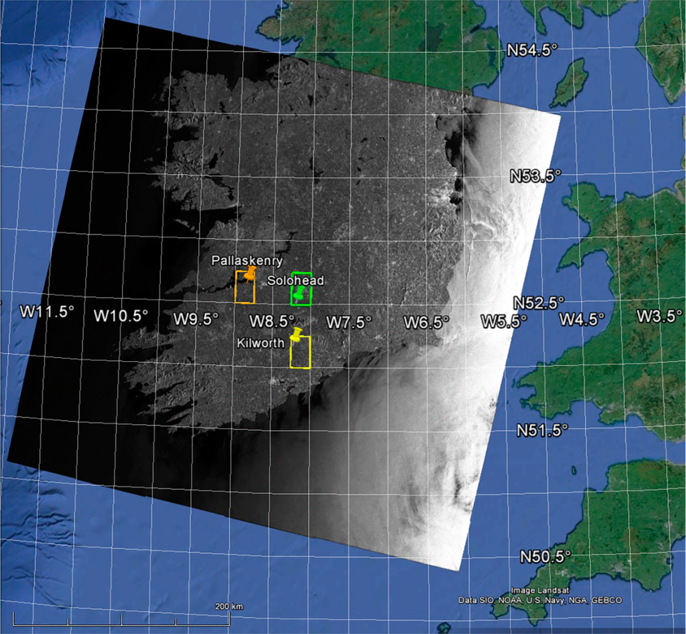
2. Test Site Description
The study focused on the south of Ireland using three in situ sites, namely Kilworth (KW), Pallaskenry (PK) and Solohead (SH) (Figure 1). The region is characterized by a humid mild temperate climate, with a mean annual precipitation of ∼1200 mm·y−1. The in situ stations are installed in grassland areas, which represent almost 80% of the agricultural area of Ireland (4.4 million hectares) [37]. The region is typically low lying, with altitudes ranging between 15 m and 104 m above sea level, and relatively flat (slope lower than 6°). On the basis of the United States Department of Agriculture (USDA), the soil texture is classified as sandy loam in Kilworth and as loam in Pallaskenry and Solohead. In Table 1, the specific characteristics of each location are reported.
3. Material and Methods
3.1. In Situ SM Data
Soil moisture in situ measurements have been collected using time domain reflectometers (TDR), Campbell Scientific CS616, installed horizontally at each of the three study sites. The instruments have not been calibrated with the soil texture, but a standard manufacturer calibration closest to the soil type has been used. This indicates that while the absolute soil moisture may not be exact, the relative soil moisture and changes of soil moisture from day to day are correct. The instrument manufacturer’s accuracy is ±2%. Measurements have been recorded at 30-min intervals, together with precipitation and soil temperature, since 2007.
The in situ instruments provide soil moisture values to a depth of 5 cm from the surface and are expressed as the soil water-filled pore space (WFPS). The ECV SM data are in volumetric units (m3·m−3). The in situ values have been converted to the same units, by using the porosity f as in Equation (1):
3.2. Remotely Sensed Data
3.2.1. ECV SM Product
In the first version of the global ECV SM product, released in June 2012, by the Vienna University of Technology (TUW) and freely available at [19], soil moisture has been retrieved from several microwave multi-frequency radiometers (Scanning Multichannel Microwave Radiometer (SMMR), Special Sensor Microwave/Imager (SSM/I), Tropical Rainfall Measuring Mission's (TRMM) Microwave Imager (TMI) and Advanced Microwave Scanning Radiometer for Earth Observation System (ASMR-E), and C-band scatterometers European Remote Sensing (ERS), Advanced SCATterometer (ASCAT)). The Water Retrieval Package (WARP) developed at TUW has been used to derive the soil moisture from active system acquisitions, while all passive products were generated using the VUA-NASA (Vrije Universiteit Amsterdam and NASA) land Parameter Retrieval Model (LPRM) software package. Secondly, two homogenized products have been generated from all of the passive and active data [38]. The error characterization of the merged passive and merged active product has been carried out through triple collocation and error propagation modelling [39]. Finally, active-passive datasets have been merged in a unique soil moisture product [16–18,40]. The rationale behind this approach is that calibration differences and other structural biases between the products in the individual product groups can be removed, before merging two products based on completely different retrieval principles. The merging procedure involves firstly rescaling the different products into common reference climatology by using AMSR-E and ASCAT-based soil moisture data as a reference. Such systems provide the most reliable climatology for the individual product groups. To supply a global coverage, a supplementary dataset is needed to scale the merged active and passive dataset into a globally-consistent climatology. Hence, the GLDAS-Noah (Global Land Data Assimilation System) data assimilation system [41] is used. Scaling is performed using cumulative distribution function (cdf) matching [16,42–44]. The drivers of the merging approach are data availability and the relative accuracy of the products.
Data availability (at a daily time step) and data sensitivity to vegetation are taken into account to combine the merged active and merged passive datasets. The average vegetation optical depth (VOD) over transitional regions (i.e., regions between sparsely and moderately vegetated areas) is calculated and used as the threshold for separating sparsely- from moderately-vegetated regions outside of the transition zones. Active soil moisture data are used for regions with moderate vegetation density (a VOD value higher than the threshold), whereas the passive product is used for (semi-) arid regions (a VOD value lower than the threshold) [38]. When, at a given location in transition zones, the correlation coefficient (R) between the merged active and passive soil moisture products is greater than 0.65, both products are used [39]. This is done by simply averaging merged passive and merged active products for time steps where both products are available; if only one product type is available, that one is used [38]. In [16], it has been shown that this procedure increases the number of observations while minimally changing the accuracy of the merged soil moisture product. Moreover, it has been observed that when the active and passive merged datasets at a given location have an R lower than 0.65, using them both reduces the quality of the merged product relative to the single products.
The SM time series maps are provided on an almost daily basis, covering a period of more than thirty years, from 1979 to 2010. The spatial resolution of the ECV SM product is approximately 0.25 degrees. Data are provided in volumetric units (m3·m−3), together with quality flags indicating the possible presence of dense vegetation, snow or a temperature below 0 °C. The ECV data used in this study are ASCAT acquisitions exclusively.
3.2.2. ENVISAT ASAR WS SM Data
The ENVISAT Advanced Synthetic Aperture Radar (ASAR) data are used in this research. The satellite was launched in 2002 by the European Space Agency (ESA), and the mission ended in April, 2012. ASAR used a C-band (5.3 GHz) SAR, which acquired images in multiple modes, polarizations and at various incidence angles [45]. In particular, the ScanSAR modes included the Wide Swath (WS) and Global Monitoring (GM) modes, covering swaths of a 405-km width under varying incidence angles. The WS mode allowed a spatial resolution of 150 m, a radiometric accuracy of less than 0.6 dB and a maximum duty cycle (the measure of the fraction of the time the radar is transmitting) of 30%, whereas the GM mode provided data with a spatial resolution of 1 km, a radiometric accuracy of about 1.2 dB and a duty cycle of 100%. Although a number of soil moisture studies have been carried out by using ASAR GM images [29,46,47], the high level of noise affecting such data led us to focus on ASAR WS products. Given their higher spatial resolution and the possibility to collect theoretically up to 3–5 images a month, ASAR WS have the potential for better characterization and monitoring of soil moisture. As regards the best geometry of acquisition for the soil moisture retrieval, previous works demonstrated that more accurate results can be achieved by considering descending orbits [48,49], whereas others by using the ascending ones [50]. However, since the combination of ascending and descending orbits allows image acquisitions of a region up to 10-times a month, both orbits were considered here. Concerning the choice of polarization, the largest amount of VV acquisitions over the region under investigation (more than 300 archive images available) led us to discard the HH-polarized data (less than 25 archive images available).
Radar backscattering mostly depends on both sensor parameters (incidence angle, polarization) and land characteristics, such as soil roughness, vegetation cover and soil moisture [51]. In particular, in the C-band, the sensitivity of the backscattering to the soil wetness decreases in the presence of vegetation [52]. However, it has been found in various studies that sparse or low vegetation cover has little influence on the backscattered signal and can generally be neglected. For example, in [53], the authors found that a grass cover (average height of 40 cm) had little influence on ERS-1 (VV polarization) backscattering coefficients, attenuating the signal by less than 0.2 dB. Since all of the study sites are cultivated with relatively short grass, the influence of the vegetation can be considered insignificant on the ASAR WS dataset.
The retrieval of soil moisture from multi-temporal SAR images has been effectively carried out in many studies with a change detection approach [54]. In this work, the change detection algorithm developed by TUW originally for ERS scatterometer images has been used [55]. It is based on the assumption of the time-invariance of surface roughness and vegetation cover, which allows differences in the backscatter to be directly related to the soil moisture variations. Such a hypothesis is met in the grassland areas under investigation, which we can assume to have undergone minimal variation during the period of observation. The original method has been successively adapted for ENVISAT ASAR GM data (1-km spatial resolution). A complete explanation of the algorithm can be found in [29], where the effects on backscattering due to varying incidence angle are taken into account by adopting a standard approach, that is the pixel-wise multi-temporal incidence angle normalization. The estimation of the maximum soil moisture retrieval error, which could affect the ASAR GM SM product, has been evaluated in [29] as:
By using the Corine Land Cover 2006 Map, the retrieved soil moisture maps have been then masked in order to exclude from the subsequent analysis pixels representing classes where the soil moisture values are not reliable (i.e., urban, evergreen broadleaf forest, water bodies, barren or sparsely vegetated areas, snow or ice). In the specific areas under investigation, only a few pixels representing water bodies in the region of Pallaskenry have been masked out. As a further indicator of the reliability of each single pixel, an additional masking has been carried out. In principle, the idea is to select only the points where the adaptation of the algorithm to the ASAR data works better. The temporal stability of soil moisture fields gives rise to an associated temporal stability in the backscatter signal [57]. A strong correlation between local and regional backscatter is usually a good indicator of high sensitivity to soil moisture dynamics at the local scale. At locations with a weak correlation, either the backscatter response to soil moisture dynamics is dominated by noise and speckle or the backscatter characteristics are adversely influenced by factors, such as dense vegetation, complex topography or soil structure/texture characteristics, which inhibit the retrieval of reliable soil moisture estimates. Therefore, for each 1 km × 1 km ASAR pixel, the correlation between the time series of the local σ0 and the average of the backscattering over the 25 km × 25 km area covering the ASAR one has been evaluated. There is no specific correlation value that is optimally applicable for the purpose of masking ASAR-based soil moisture products in general, as this value depends on backscattering mechanisms, environmental conditions and on the requirements of the intended application of the soil moisture data. In this study, a threshold of R2 = 0.3 was set based on the mentioned assumptions and the experience of other researchers working with ASAR data [58]. After the masking process, it has been observed that in all of the sites, the classes cropland/grassland mosaic and pastures occur over 90% of the ECV pixel areas.
In order to compare the soil moisture expressed by the same unit (m3·m−3), the ASAR relative SM index values have been transformed by applying Equation (1).
3.3. Regional Scale Analysis of SM Temporal Variability
The ECV SM product was compared, on a regional scale basis, with the finer spatial resolution ASAR WS SM data and with the ground measurements. Bearing in mind the different temporal frequency of each dataset, only the ECV and in situ SM data corresponding to the ASAR WS acquisitions dates have been considered. The absolute soil moisture values derived from each sensor and their relative changes over time have been considered. This study mainly focused on the latter, aiming at an understanding of the capability of the ECV SM product in capturing soil moisture temporal variations.
The geographical position of the in situ stations has been plotted on a georeferenced grid, and the surrounding regions that exactly coincide with the ECV pixels have been selected. Because of the masking process, the number of ASAR data in each ECV pixel is lower than the maximum obtainable. Specifically, when the ECV pixels are completely covered by the ASAR acquisitions, the percentage of available ASAR pixels in each site is: 92.1% for Kilworth, 80.5% for Pallaskenry and 94.7% for Solohead. Moreover, because of the variability of the ASAR coverage over the areas of interest, the number of accessible soil moisture values can change significantly in each acquisition taken during the period of observation. In order to make the subsequent analysis statistically consistent, only the ASAR acquisitions that cover the ECV pixels for more than the 50% of the available pixels (after masking) were considered in the study. For each ASAR acquisition, the average of the soil moisture values retrieved within the corresponding ECV cell has been taken into account for the dataset comparison.
At first, ascending (A) and descending (D) ASAR acquisitions (soil moisture and backscattering) were compared separately with the ECV and in situ soil moisture values. The number of ASAR data temporally compatible with the other two datasets is reported in Table 2. Subsequently, two more studies have been carried out: in the first experiment, the whole set of ASAR WS data (AD) has been used together, whereas in the second one, ascending and descending SM values referring to the same day have been averaged ( ).
The in situ SM values have been estimated by adopting two different approaches:
Only the soil moisture measurements recorded at the time closest to the ASAR acquisitions have been used.
The soil moisture values have been evaluated on a daily basis, by averaging the measurements recorded from 0:00 to 23:30 of the same day as the ASAR acquisition.
Summarizing, according to the different approaches, seven comparisons have been performed between the ECV SM product and the other two datasets. Specifically:
A_A: only ASAR ascending acquisitions, Approach A for the in situ values;
A_B: only ASAR ascending acquisitions, Approach B for the in situ values;
D_A: only ASAR descending acquisitions, Approach A for the in situ values;
D_B: only ASAR descending acquisitions, Approach B for the in situ values;
AD_A: both ASAR ascending and descending acquisitions, Approach A for the in situ values;
AD_B: both ASAR ascending and descending acquisitions, Approach B for the in situ values;
: both ASAR ascending and descending acquisitions, averaging the ASAR and the in situ soil moisture values on a daily basis.
In addition, a seasonal comparison has been also carried out between the three datasets, aiming at evaluating the performance of ASAR and ECV soil moisture products in capturing the annual cycle of surface SM and its short-term variability. Since it has been demonstrated that the seasonal vegetation C-band signal is much weaker than the soil moisture signal [59], its effects are generally neglected in the retrieval algorithms [49]. However, the vegetation cycle or intense precipitation periods may reduce the quality of satellite soil moisture products. Therefore, long time series have been split into four seasons (i.e., winter (DJF), spring (MAM), summer (JJA) and autumn (SON)) and analysed in comparison with the in situ measurements, which are considered as a reference for the product quality assessment.
The Pearson correlation coefficient (R) has been used to characterize the temporal agreement between each dataset (ECV, ASAR, and in situ) at each test site. However, due to the limited number of collocated measurements (approximately 100 for the annual analysis and consequently only around 25 for the seasonal analysis), a certain chance exists that the obtained correlation levels are achieved by coincidence rather than a real statistical dependency. The null hypotheses of the non-significant correlation was tested using the Student’s t-test, which relates the correlation value to the number of measurements used to calculate it, in order to estimate the probability (p-value) of the achieved correlation to be a coincidence, i.e., not significant. The used threshold for accepting the null hypotheses was 0.025 (i.e., 2.5% chance for a statistical coincidence). It should be emphasized that statistical significance does not mean that the correlation is high, but that the correlation estimate is reliable.
3.4. Analysis of SM Spatial Variability
Heterogeneity of terrain, vegetation cover and topography can make the soil moisture extremely variable even over small distances [60], a variability that the coarse spatial resolution of the ECV SM product may mask. Previous studies [61–63] used soil moisture measurements recorded in several in situ stations aiming at the understanding of soil moisture variability over relatively small distances. However, contradictory results have been found, highlighting the complexity of the phenomenon and thus the difficulty of accurately predicting the dynamics of the soil moisture in different areas.
In this work, the SM spatial variability has been studied at the resampled ASAR scale (1-km spatial resolution after resampling). The aim is to investigate which geophysical factors (e.g., terrain composition, altitude, land cover) mainly affect the representativity of the ECV SM product.
Firstly, the average of the soil moisture retrieved from the ASAR WS acquisitions over each ECV-sized cell has been compared with the coefficient of variation (CV) expressed as:
Successively, the ASAR SM time series values recorded in each pixel have been compared with the ECV SM data. Finally, correlation maps have been provided also on a seasonal basis. The objective of this analysis was to investigate the correlation patterns within the ECV cell and their relationship with specific soil characteristics in terms of texture, land cover and altitude.
3.5. Error Characterization
A statistical approach has been used to quantify the error terms, by computing the root mean square difference (RMSD). This signifies the closeness of two independent datasets representing the same phenomenon. Because of the complexity of the soil moisture phenomenon and the different spatial scale representativity, none of the investigated datasets can be assumed to be the truth, although the in situ measurements are normally considered as the reference. As a consequence, the RMSD does not provide a measure of accuracy, but represents the relative error of the soil moisture dynamic range [64]. The RMSD varies with the variability within the distribution of error magnitudes and with the square root of the number of data, as well as with the average-error magnitude (MAE) [65]. Since the ASAR, and the in situ SM values are expressed in degrees of saturation, while the ECV SM product is given in volumetric soil moisture; and because of their different spatial resolution, the RMSD is generally affected by a bias. Therefore, all of the SM datasets have been expressed in the same unit (m3·m−3), and the bias has been removed, achieving a better and more reliable estimate of the error by evaluating the centred (unbiased) RMSD:
4. Results
4.1. Soil Moisture Temporal Variability
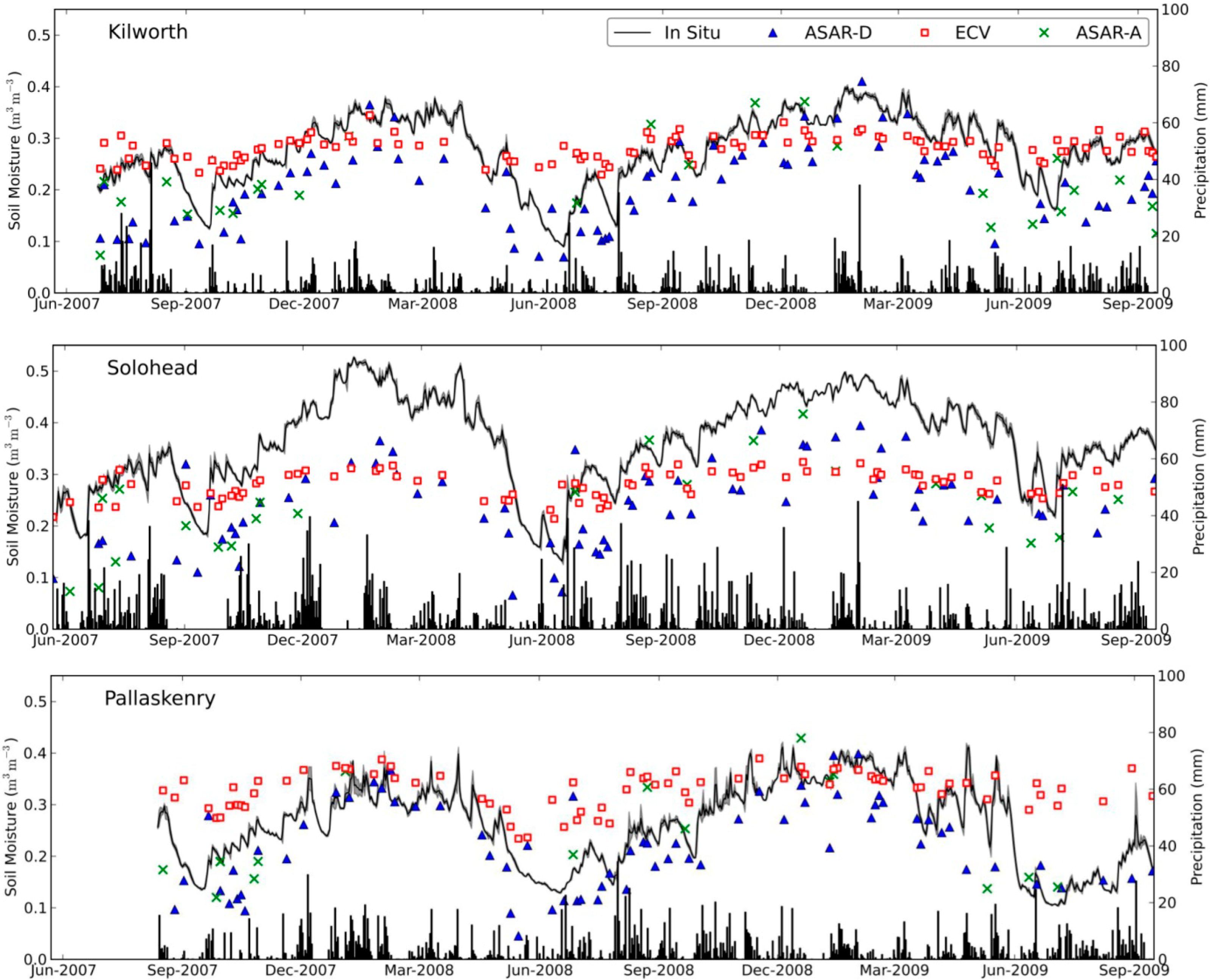
In Figure 2, the soil moisture time series retrieved from ascending and descending ASAR WS acquisitions are shown with the ECV values and the in situ continuous measurements. The accumulated daily precipitation values are displayed in Figure 2.
Comparable trends are seen for Kilworth and Pallaskenry, where the ECV SM values are about 25% and 31% greater than those retrieved from ASAR, respectively. For Pallaskenry, there is good agreement with the temporal trend of the in situ measurements. While the ECV SM varies in a relatively small interval (0.1 m3·m−3), a more significant temporal variation occurs in the ASAR time series. The same behaviour is much more evident in the in situ measurements, which vary in an interval of approximately 0.25 m3·m−3. Generally, the ECV SM values tend towards the highest in situ values. On the contrary, the driest ground conditions are not well represented by the ECV product. Such an observation confirms what has already been shown in other studies [66], where in situ measurements and the soil moisture derived from scatterometer acquisitions have been compared. The bias between ASAR and ECV soil moisture is smaller in Solohead, while neither dataset follows the temporal variation exhibited by the in situ time series. In this case, the ECV SM values vary in a small interval (0.21–0.32 m3·m−3) below the average of the soil moisture ground measurements (0.35 m3·m−3) recorded during the period under investigation. Contrary to the other two sites, here the best agreement between absolute SM values (ECV, ASAR and in situ) occurs in the driest conditions. Such a different behaviour of the soil moisture may be explained as a consequence of the low infiltration capacity of the clay, whose percentage is larger in the soil at Solohead than in the other regions studied. The comparison between the soil moisture retrieved from the remote sensing acquisitions and the in situ measurements show very similar results for both approaches, “A” and “B”. The daily standard deviation of the in situ values for all sites is 0.006 on average. This means that the variation of soil moisture during the day is negligible. Therefore, the value recorded at the time of the ASAR acquisition (Approach “A”), does not differ significantly from the daily mean (Approach “B”).
Moreover, in terms of correlation and error (Tables 3 and 4), the results are essentially independent of the choice of the ASAR dataset (ascending, descending or both of the acquisitions). It should be noted that the number of ascending acquisitions is much smaller than the number of descending ones. In general, a lower degree of correlation occurs when only the ascending ASAR SM time series are used, with the exception of Pallaskenry. However, statistically significant correlation levels (p < 0.025) and low unbiased RMSD (ubRMSD) between the independent and multi-scale soil moisture time series have been noted in all of the sites. Specifically, the ASAR vs. ECV SM analysis demonstrate high correlations (KW: R = 0.76–0.77, PK: R = 0.72–0.79, SH: R = 0.77–0.88), associated with a quite low ubRMSD generally equal to 0.06. High agreement has been found between the ASAR and in situ SM time series, with a degree of correlation larger than 0.71 and ubRMSD ranging between 0.05 and 0.06, with the only anomaly being the ascending ASAR SM data at Kilworth. Probably due to the spatial scale difference, the worst outcome in terms of correlation has been estimated between ECV and in situ SM data. Nevertheless, R is still quite high (generally higher than 0.6), and the ubRMSD varies in the interval 0.04–0.06.
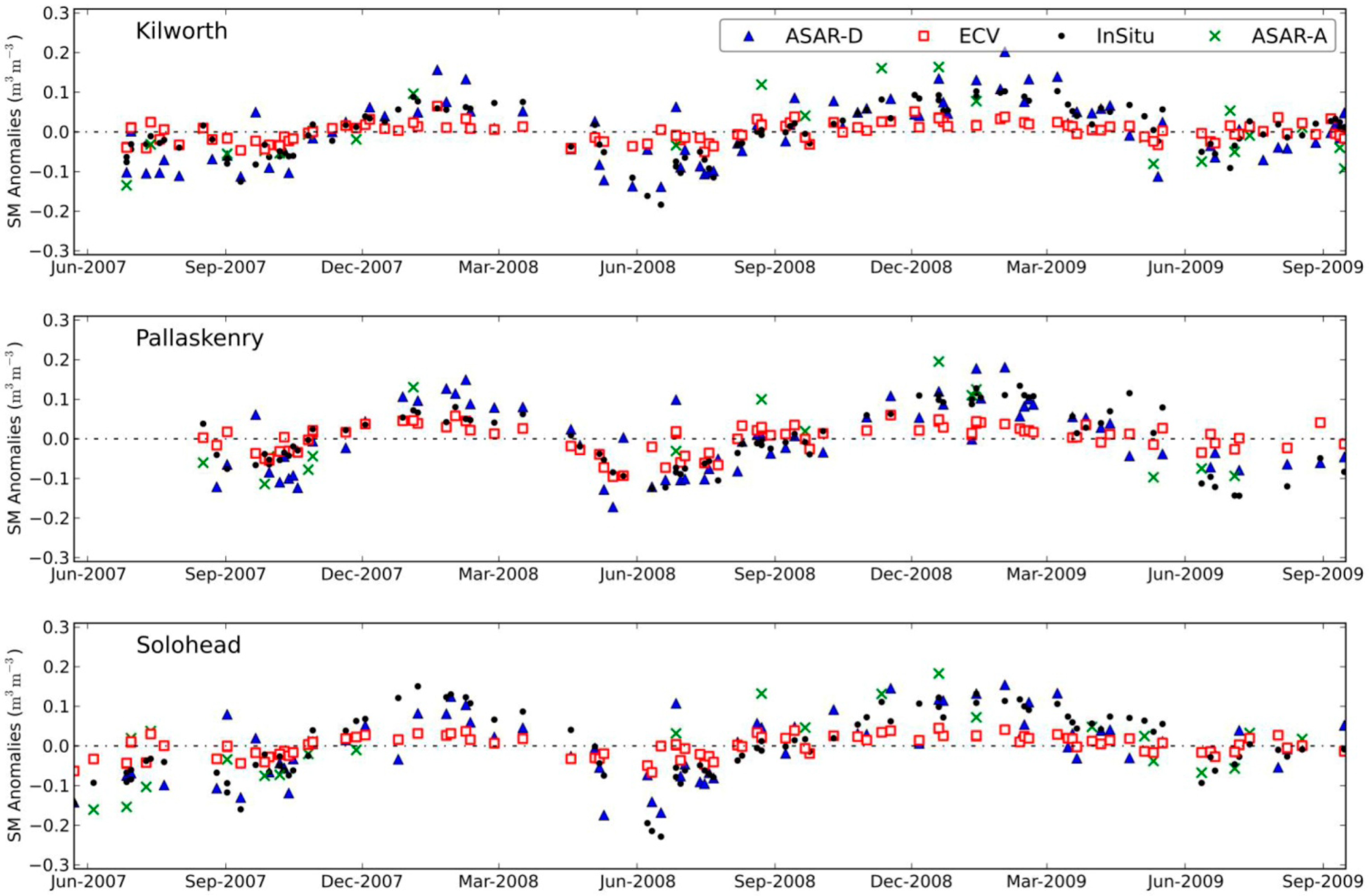
Soil moisture anomalies have been estimated for all three datasets, during the time interval 2007–2009 (Figure 3). The seasonal cycles are well represented by the temporal evolution of the ASAR and in situ SM anomalies, which exhibit similar positive higher values in winter and negative lower values in summer. On the other hand, the poor variability of the ECV SM data leads to a very small range of variation of the associated anomalies. Despite the short period of observation (about two years), it is still possible to detect atypical moisture conditions through the analysis of ASAR and in situ SM anomalies. Specifically, in 2007, a drier autumn occurred at all sites compared to 2008. Based on the in situ measurements, in Kilworth and Solohead, the summer of 2008 was drier than the previous and following year. While ASAR SM data are able to capture such a condition, the ECV SM product does not detect any significant anomaly. In Pallaskenry, similar dry soil conditions are revealed by the computation of in situ, ASAR and ECV SM anomalies. Successively, in 2009, a wetter summer occurred in Kilworth and Solohead, where the SM anomalies estimated by using all three datasets are very close to zero, meaning that the soil moisture was close to the average evaluated over the whole period of observation (2007–2009). In Pallaskenry, the in situ and ASAR anomalies are similar to those recorded in the summer of the previous year; however, the ECV SM anomalies hover about the null value, thereby suggesting wetter conditions compared to the previous summer.
4.1.1. Seasonal-Based Analysis
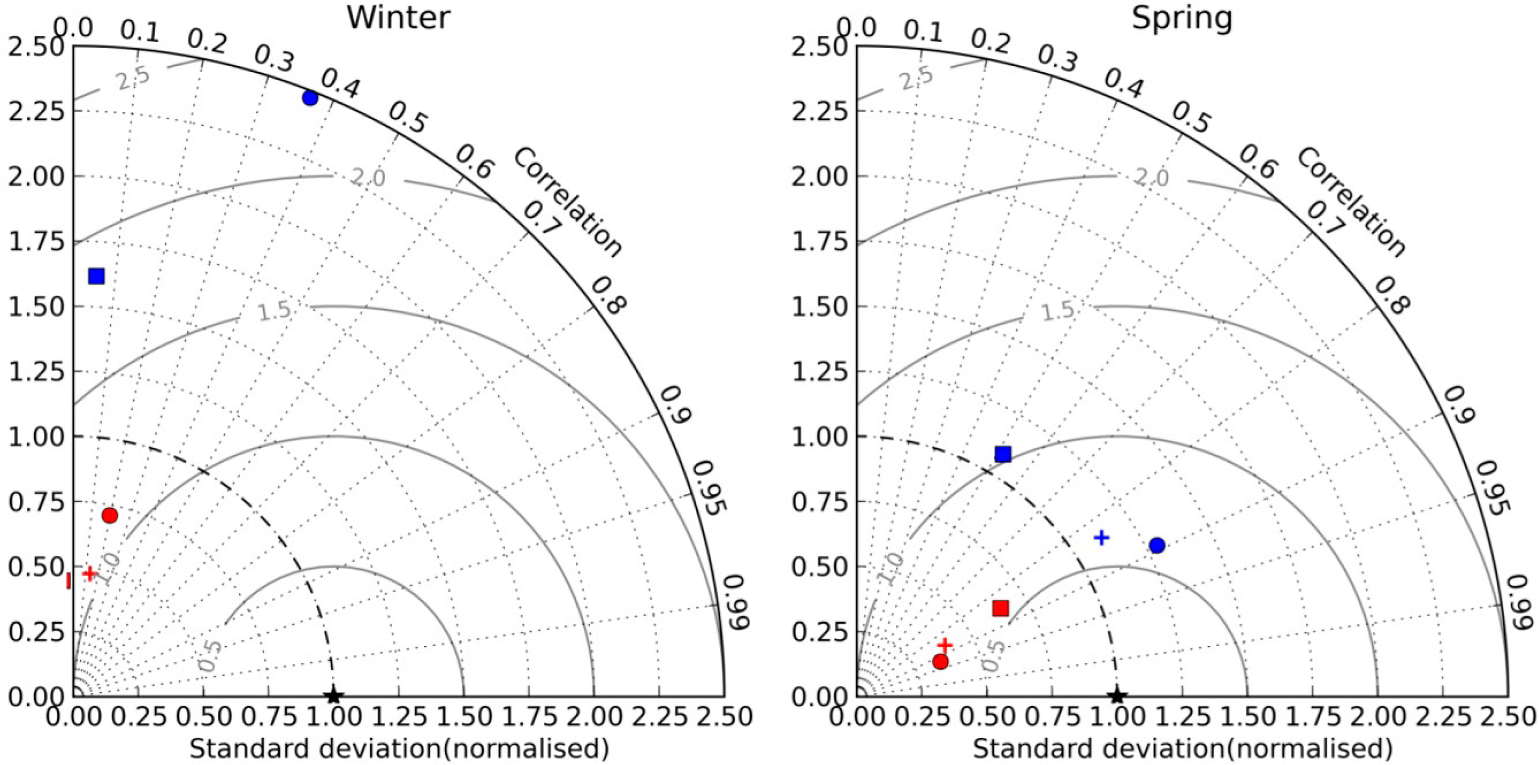
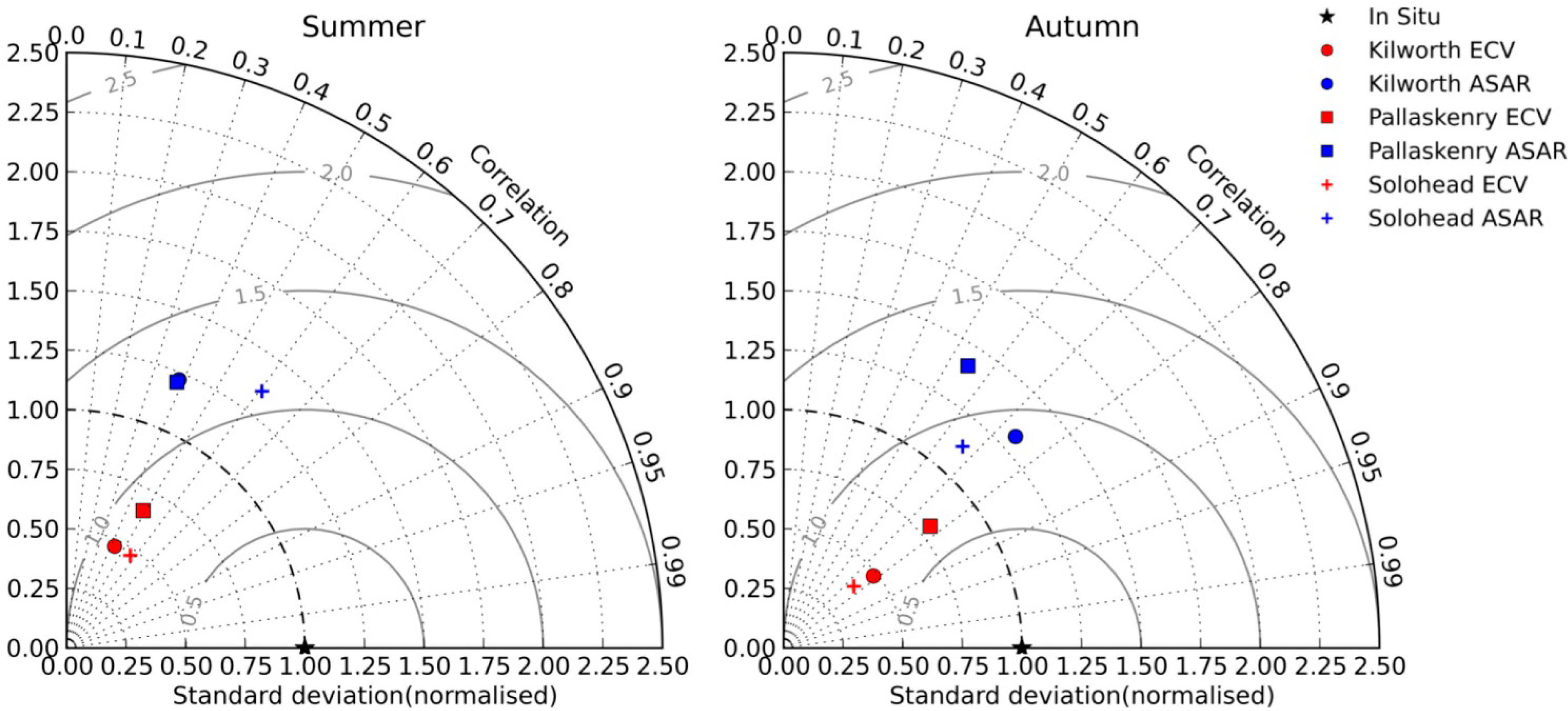
To investigate the ability of ASAR and ECV SM products to capture the annual cycle of surface SM and its short-term variability, a seasonal comparison has been carried out. For each dataset comparison, the correlation R, the unbiased RMSD and the normalized standard deviation (SDV) have been estimated and plotted in the Taylor diagrams in Figure 4. The normalized standard deviation is defined as the ratio between the standard deviations of soil moisture product and in situ measurements:
The best agreement between the different remote sensing SM products and the in situ measurements occurs at a short distance to the R = 1, SDV = 1 point.
4.1.2. ASAR vs. In Situ SM
The seasonal Taylor plots in Figure 4 with the ASAR SM symbols, always located on the right side of the arc with a radius equal to one, highlight the larger variability of the ASAR SM mean with respect to the local in situ measurements. For both Solohead and Kilworth, the highest correlation value occurs in spring (MAM), with the poorest agreement in winter (DJF) and summer (JJA) (Figure 4). For Pallaskenry, similarly high correlations are seen in autumn (SON) and spring, while the lowest correlation occurs in winter (Table 5). However, in this case, the p-value is 0.4, making the analysis statistically unreliable. The seasonal-based analysis shows the poorest agreement generally occurring in Pallaskenry (Table 5).
Concerning the error estimation, no significant seasonal variations are seen across the sites. In fact, the ubRMSD ranges between 0.03 and 0.06. The only exception occurs in Solohead, where higher values (0.07–0.08) are observed in all the seasons, except in winter.
4.1.3. ECV vs. In Situ SM
As the ECV SM symbols are always on the left side of the arc with a radius equal to one (Figure 4), this indicates that the ECV values are less variable than the in situ measurements. The seasonal comparison between ECV and in situ SM data (Table 6) confirmed what has been generally found in the previous analysis: the best agreement is achieved in spring and the worst in winter at all sites. However, the results of the analysis carried out for the winter datasets are characterized by high p-values, indicating less statistical reliability. At the same time, low correlation values, with p < 0.025, have been observed also in summer. This suggests that the retrieval algorithm may be sub-optimal in very wet or in the driest conditions.
The highest ubRMSD occurs in spring, varying between 0.05 and 0.06. However, no significant variations are noted in the other seasons and in every site. (Table 6)
4.1.4. ASAR vs. ECV SM
Regarding the ASAR-ECV SM comparison (Table 7), the highest correlation values are in spring in the Kilworth and Pallaskenry sites and in winter in Solohead. The lowest correlation values are in winter for Kilworth and Pallaskenry and in summer for Solohead. Different to the previous comparison, the correlation between ASAR and ECV SM datasets is less sensitive to the season. The highest variability in the seasonal R values can be observed in Kilworth (R = 0.62–0.84), whereas an even smaller range of variation has been evaluated for Pallaskenry (R = 0.53–0.66) and Solohead (R = 0.70–0.78). As the p-values are lower than 0.025, all of the results can be regarded as statistically reliable.
Regarding the ubRMSD, the lowest errors occur in winter in all of the sites, although in Kilworth, the same value has been found in summer. In other seasons, there is minimal or no variability at all sites.
4.2. Soil Moisture Spatial Variability
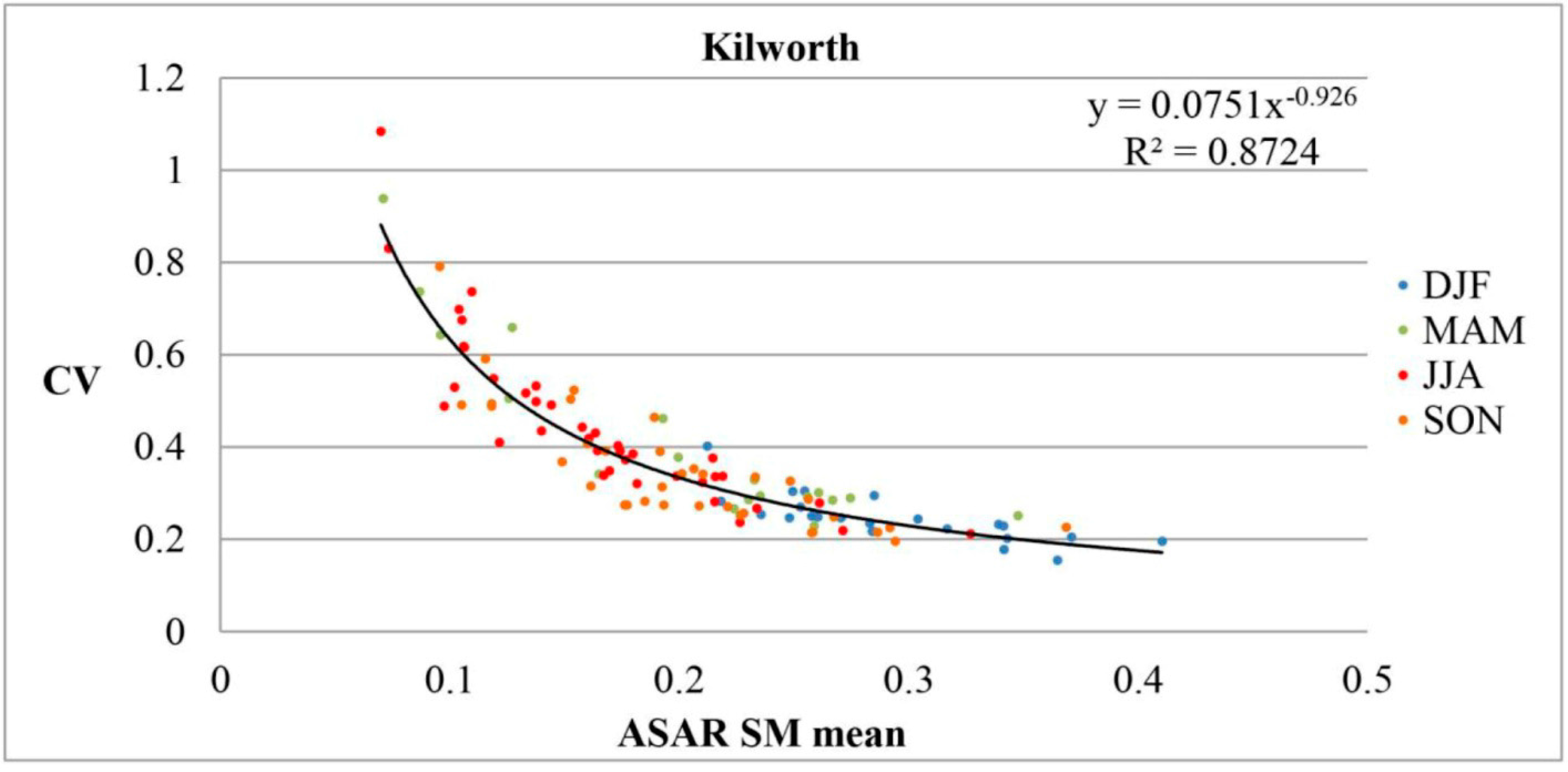
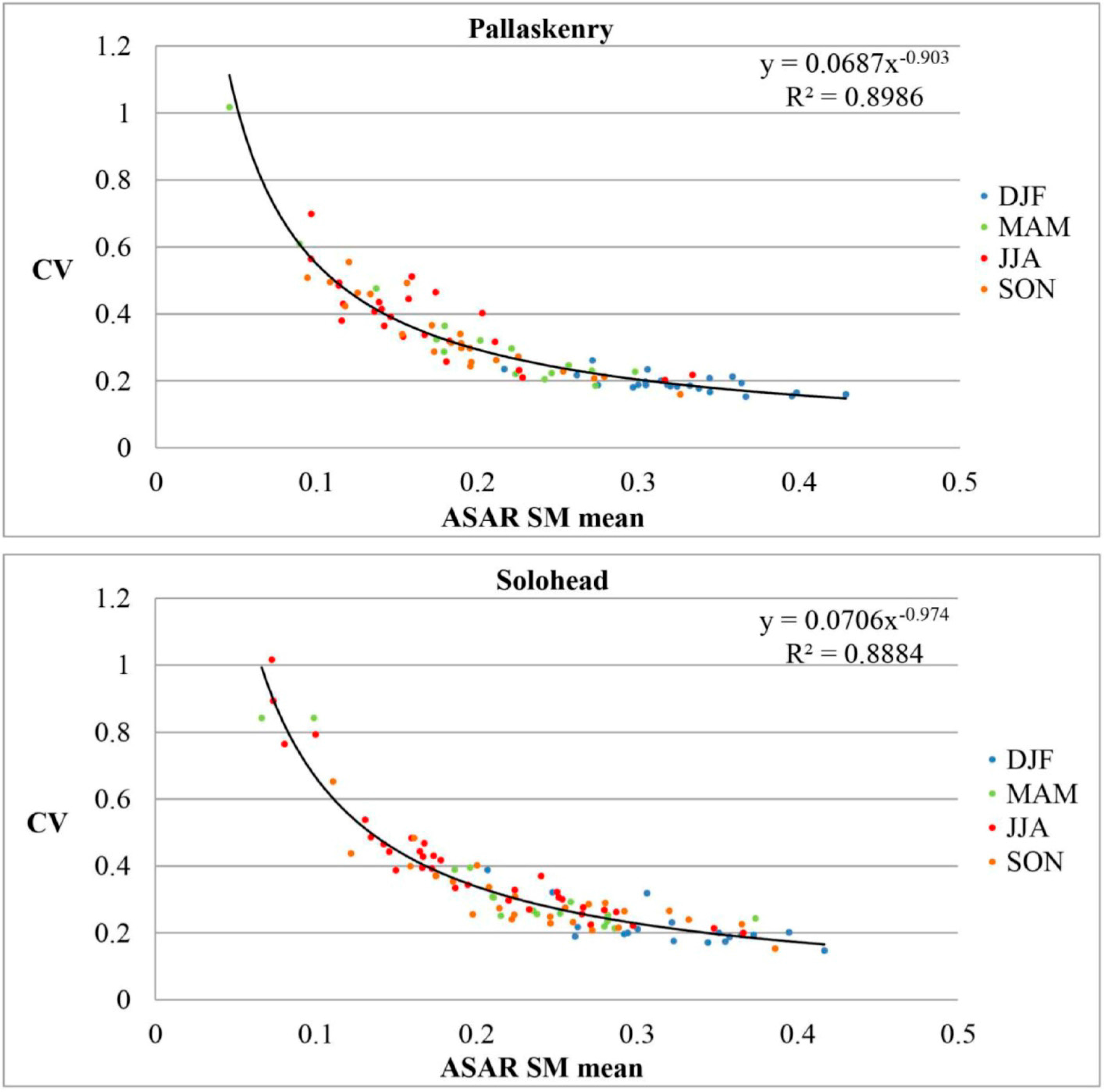
As a measure of the spatial variability of the soil moisture, for each ASAR acquisition, the coefficient of variation (CV) has been plotted as a function of the mean of the SM (Figure 5). Furthermore, seasonal values are highlighted with different colours. In wetter conditions, the soil moisture is less variable for all sites. As a consequence, in winter, the soil moisture is more homogeneously distributed, whereas in summer, high spatial variability occurs. The trend of the CV approximates a decreasing power function, with a high coefficient of determination (R2 > 0.87). Our results agree with the findings reported in [60]. However, it can be observed that, above values of 0.2 m3·m−3, the CV tends to vary linearly with the mean of the soil moisture, as reported also in [67,68].
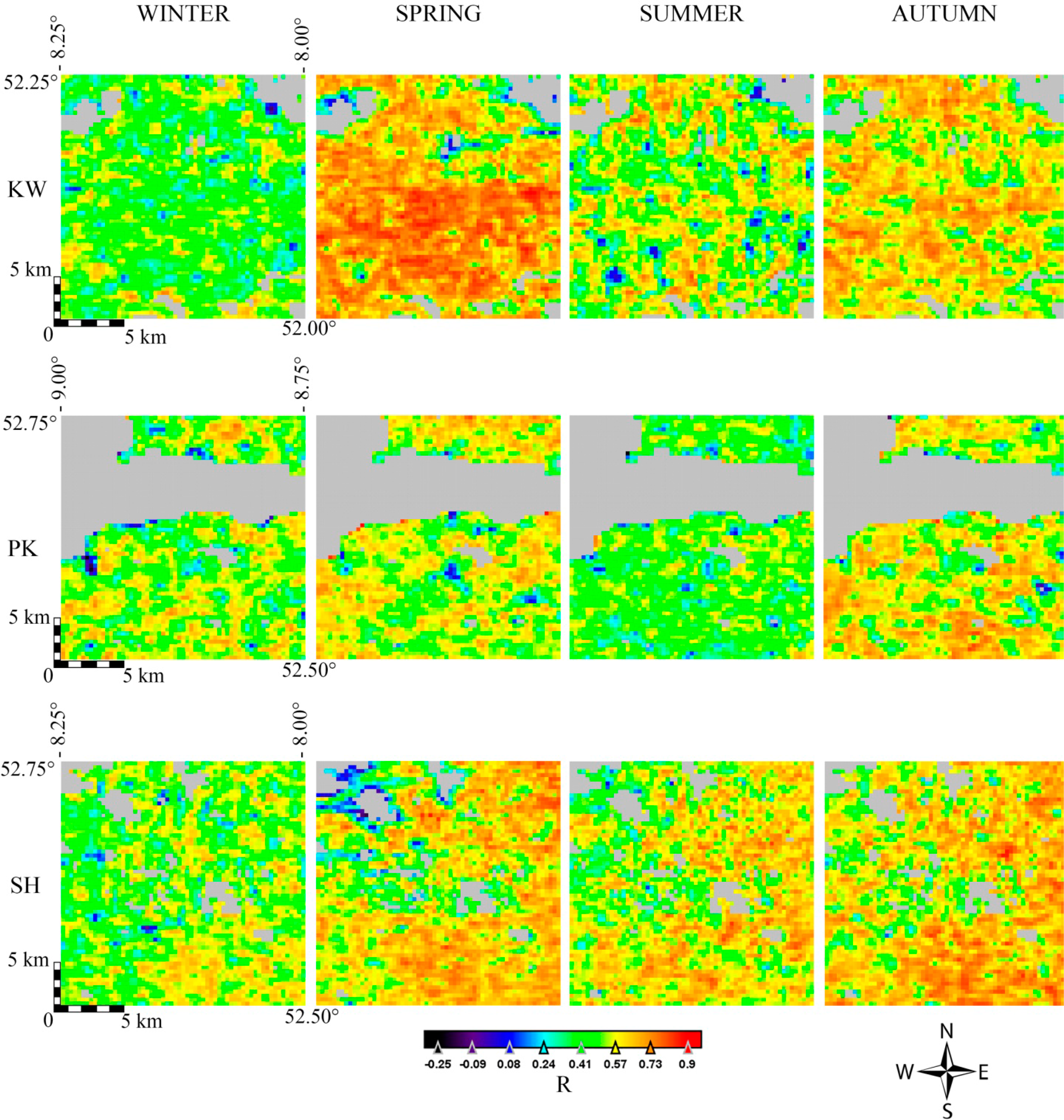
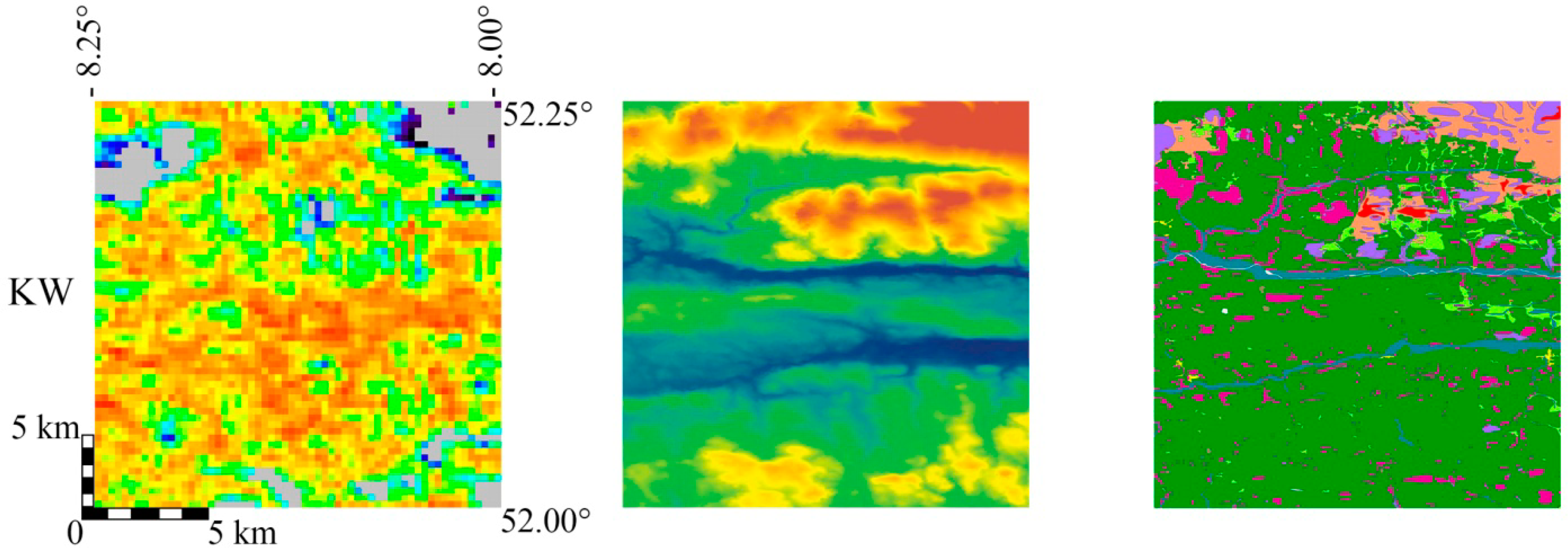
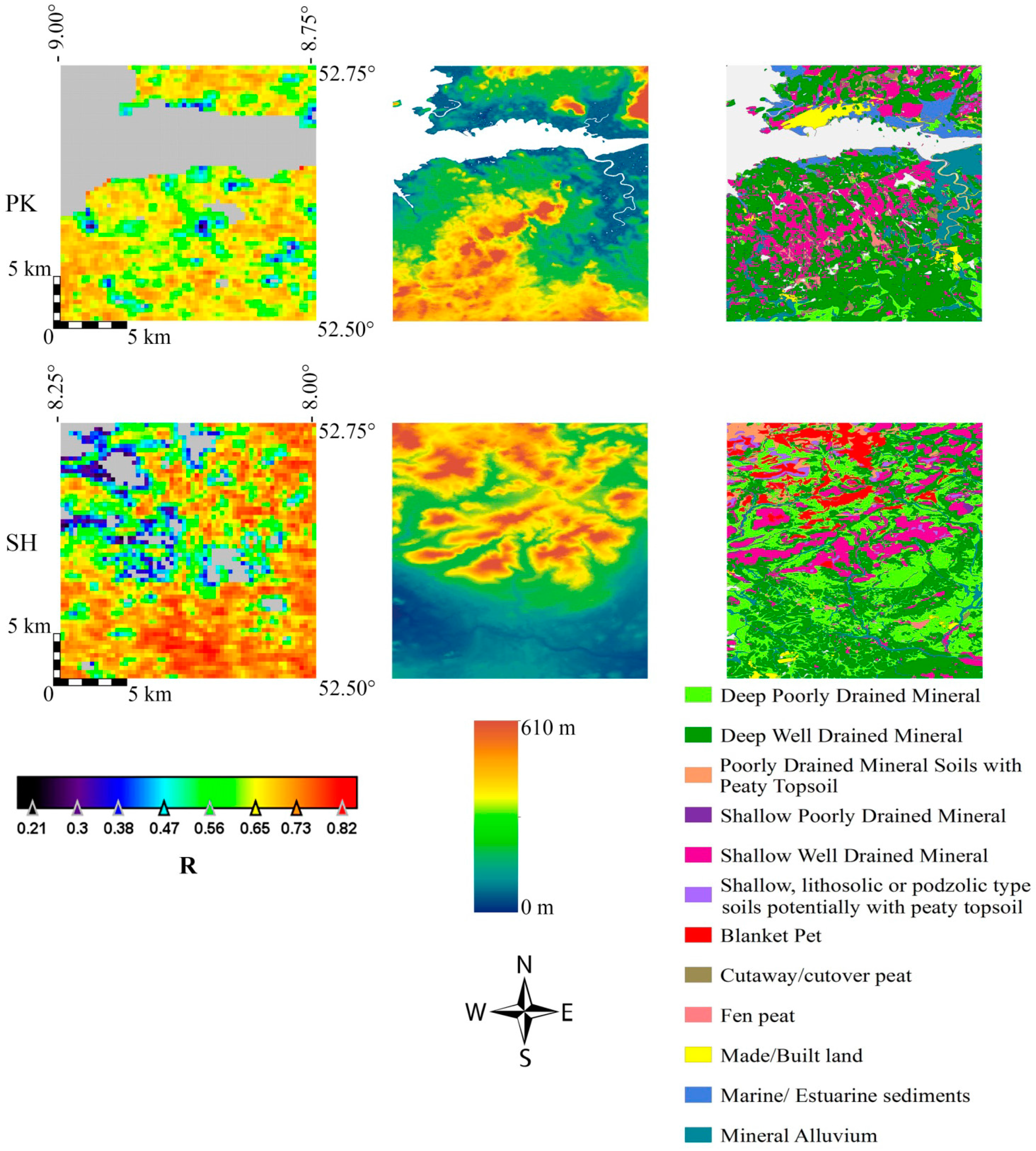
Each ASAR SM local time series value has been successively correlated with the ECV SM data (Figure 6, left). In general, there are quite high R values across all three sites. The highest correlations are seen in Kilworth and Solohead, although the top left corner of the Solohead ECV-sized pixel has quite a low correlation. The comparison with the DEM and soil maps (Figure 6, middle and right) highlights the influence of the combination of altitude and soil type on the soil moisture variations and, hence, on the representation of the ECV SM product. The soil moisture behaviour over those areas characterized by lower altitudes is better described by the ECV SM dataset (high correlation values). These regions mainly correspond to zones where the soil type is classified as deep, well-drained, mineral and mineral alluvium.
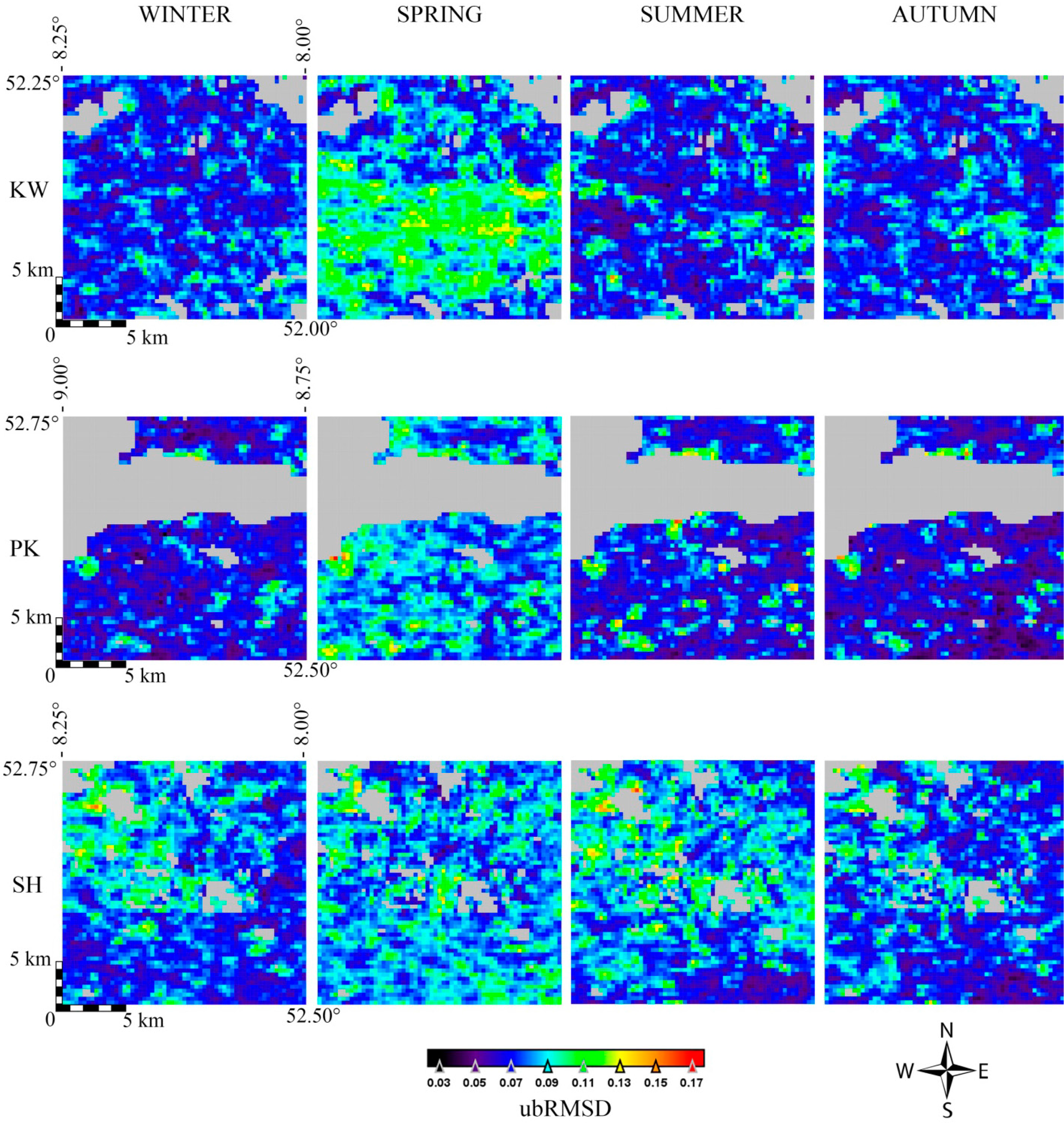
The soil moisture spatial analysis has been carried out also on a seasonal basis. The correlation and ubRMSD values between ASAR SM time series collected in each 1 km × 1 km pixel and the ECV SM dataset are shown in Figures 7 and 8, respectively. A seasonal cycle of the correlation can be noted: in the spring and autumn seasons, the highest values are reached; in summer, R exhibits lower values, as well as in winter. Conversely, the seasonal ubRMSD shows a different behaviour, with higher values generally occurring in spring. In the other seasons, no significant variation of the ubRMSD can be observed. Such seasonal variation is slightly different in Solohead, where high and more homogenously distributed ubRMSD values occur in spring and summer, while generally lower values can be observed in winter and autumn in most of the ASAR pixels.
5. Discussion
As a contribution to the validation of the innovative CCI-ECV SM global product, in this work, a triple way comparison has been carried out for the first time for such a long time series of SM observations collected using different sensors and provided at very different spatial resolution. The results achieved by comparing the three soil moisture datasets temporally and spatially demonstrate the capability of the ECV SM product in representing the soil moisture variability, despite its coarser spatial resolution. The comparison of the ECV SM product with the ASAR WS and in situ time series has shown the capability of the former to capture the temporal dynamics of soil moisture in all three test sites. The ECV SM dataset is highly correlated with the finer spatial resolution ASAR SM product and with the in situ measurements. Such outcomes are consistent with the results obtained in previous works. For instance, in [20], the authors related ECV SM data and in situ measurements taken at several stations worldwide, representing different climate zones and characterized by different topography, but mostly located over grassland or agricultural fields. They found correlation values ranging between 0.5 and 0.7 and ubRMSD equal to 0.05–0.06, which are in agreement with what has been observed in the present study. In [50,69], correlation values calculated between ASCAT SM and in situ values taken in humid regions are similar to those calculated here between ECV SM data (in our work, generated by using only ASCAT acquisitions) and in situ measurements. Our results also agree with those in [29], where the soil moisture retrieved from ASAR GM acquisitions has been compared with that derived from ERS scatterometer data and in situ measurements.
It should be noted that the lowest correlations have been estimated when only ascending (10:00 pm) ASAR acquisitions have been used, while improved outcomes have been achieved by using images taken during the descending orbit (10:00 am). Similar findings have been reported in other papers, where ASCAT- and/or AMSR-E-derived SM data have been analysed [50,69,70]. For instance, in [69], the authors suggest the use of morning measurements, because of the day-time decoupling that could happen in the afternoon due to the non-hydraulic equilibrium of the soil.
By analysing the satellite soil moisture values, it has been observed that those provided by the ECV product are generally higher than those derived from the ASAR WS acquisitions. The reason may be related to the change detection algorithm used to retrieve the soil moisture from the SAR images. It is based on parameters that have been shown to be sensitive to the season [71] and on assumptions derived from the use of SM time series by ERS scatterometer data [29]. Nevertheless, we have demonstrated here that ASAR WS data are suitable to assess the quality of the coarser spatial resolution ECV SM product. By considering the in situ soil moisture dataset as the reference, high correlation values and small bias have been estimated between ASAR SM time series and the ground measurements.
The comparison between the three soil moisture datasets shows that the temporal variability of the ECV SM product is lower than for the ASAR SM and in situ data, as noted previously in [20]. The different spatial scale of the SM products used may lead to such a behaviour [29]. In particular, the processing performed to generate the ECV SM data, which are scaled to the GLDAS-Noah model, yields a coarser spatial resolution with a limited ability to track the seasonal soil moisture variability. At the same time, the absolute SM values variations are reduced throughout the whole period of observation. In this regard, the analysis of the soil moisture anomalies during approximately two years of observations has shown a seasonal periodicity, which is particularly evident in the ASAR and in situ SM datasets, rather than in the ECV SM time series. Higher anomalies have been observed in winter and lower ones in summer. Specifically, the ASAR and in situ soil moisture products highlight the occurrence of anomalous dry and wet summers in Kilworth and Solohead in 2008 and 2009, respectively, whereas the ECV SM product fails to capture dry extremes. However, it should be noted that anomalies were calculated with respect to just over two years of data. For this specific study, only ASCAT data were available to generate the ECV product. As has been already observed in [66], in the driest conditions, the SM retrieved from only scatterometer acquisitions tends to overestimate the real moisture content as measured by in situ instruments. The very small anomalies of the ECV SM time series reflect this trend. The poor capability of the ECV SM product in capturing the driest and wettest soil conditions has been highlighted also in a seasonal-based analysis. It demonstrated that very low correlations occur in winter and summer between both satellite products and the ground soil moisture dataset, whereas the best agreement has been achieved in spring and autumn. Winter is the wettest season in Southern Ireland. When heavy and/or continuous precipitation occur over a poorly-drained soil (e.g., Solohead), a water layer could persist on the surface, reducing the satellite microwave backscattering sensitivity to soil moisture and, hence, providing incorrect estimates of the moisture content. Summer is the driest season, during which the vegetation reaches the maximum growth, which may affect the quality of the retrieved soil moisture from SAR and scatterometer images. Furthermore, when the change detection algorithm is applied on humid sites by using a limited number of images, the sensitivity of the microwave signal to soil moisture (the difference between the driest and wettest signal) is likely to be underestimated [72,73]. This can explain the low correlation between ASAR and in situ SM data in winter and summer.
Concerning the soil moisture spatial variability study, while published works are typically carried out through geostatistical analysis by using hydrological models and in situ networks over rather wide regions, in this work, the spatial distribution of soil moisture has been investigated at the ASAR scale (1 km) within a smaller area (i.e., the ECV size pixel). In doing so, actual observations covering the whole area have been used, without the need for adopting any particular model. This approach facilitated an understanding of the extent to which geophysical factors, such as soil texture, terrain composition and altitude, affect the retrieved ECV SM product values in temperate grasslands. The spatial variability of the soil moisture retrieved from the ASAR WS acquisitions over each ECV-sized pixel shows that wet conditions lead to more homogeneous moisture content across the area, while in the driest conditions, a significant variation in soil moisture values can occur. Therefore, in winter, the distribution of soil moisture is rather homogenous over the ASAR pixels within the ECV cells. On the contrary, a larger spatial variability has been observed in summer. This may be due to the frequent, but localized, heavy shower activity, which characterizes summer in Ireland. Under such conditions, the combination of soil texture type, terrain composition, evapotranspiration and percolation processes and water table levels is likely to play a significant role in the soil moisture dynamics. In the present work, we have been able to demonstrate how CV varies against the ASAR mean values for a full range of moisture conditions, and this highlights the seasonal variability. The trend of the CV approximates a decreasing power function, with a high coefficient of determination (R2 > 0.87). Winter mean soil moisture values are associated with the lowest and most stable CV. On the contrary, summer mean soil moisture values correspond to high and more variable CV values. Our results agree with the findings reported in [60], where the authors described the SM spatial variability for different types of soil texture. In particular, the authors note that the CV of sandy soil increases as the soil dries and reaches its maximum near the residual moisture content. However, it can be observed that above values of 0.2 m3·m−3, the CV tends to vary linearly with the mean of the soil moisture. This result is in line with [67,68], where, focusing on soil moisture behaviour in humid grassland, the authors found the relationship between CV and the mean soil moisture to be a decreasing linear function. In [74], the authors observed that in wet catchments in New Zealand, the variability decreases with increasing moisture content, whereas it increases in the drier Australian catchments. They assert that these differences in behaviour are due to differences in the seasonal patterns of controlling processes associated with seasonal changes in spatial mean soil moisture, particularly the lateral flow processes, which are related to climatic differences. Our results underline the ability of ASAR WS retrieved SM data to track this full spectrum of varying moisture content and seasonal behaviour.
The comparison between soil moisture time series in each ASAR pixel and in the corresponding ECV cells has shown high R values, larger than 0.56 on average at all sites. This highlights the effectiveness of the ECV SM product in representing the soil moisture conditions, despite the coarse spatial resolution. A further confirmation of the quality of the ECV SM product is given by the fact that the seasonal R values are quite homogenously distributed over all sites, following the same periodic trend observed by carrying out the regional based analysis (higher R values in spring, lower in winter). By studying the spatial distribution of the correlation between ASAR and ECV SM, it has been observed that the soil moisture behaviour over those areas characterized by lower altitudes is better described by the ECV SM dataset (high R values). These regions mainly correspond to zones of deep, well-drained, mineral and mineral alluvium soils. On the contrary, areas located at a higher altitude, mainly characterized by poorly-drained soil, show lower correlation between the two satellite SM products. In addition, high slope variability contributes to the further loss of correlation. Indeed, infiltration, drainage and runoff depend on the slope angle. Steeper slopes generally cause lower infiltration rates, rapid subsurface drainage and higher surface runoff [75]. Since ASAR WS acquisitions are not necessarily taken at the same time as the ECV satellite data, different moisture content is likely to be detected by each product over these regions. The lower spatial correlation observed in Pallaskenry, which is characterized by a more complex topography and higher altitude, supports such a hypothesis.
6. Conclusions
The representativeness of the global soil moisture product provided in the framework of the ESA CCI programme has been investigated through the use of finer spatial resolution ASAR WS data and ground measurements across three grassland sites in Southern Ireland. In doing so, this is the first time a comparison has been carried out between three sets of independent observations from different sensors at very different spatial resolutions for such a long time series. Neither dense in situ station networks, nor hydrological models have been used, but the results obtained from the adopted approach are consistent with those reported in other papers using different sensors and classical methods. Therefore, the applicability and reliability of the approach presented has the potential to be an efficient and cost-effective validation method for low resolution SM products.
Both the regional-based and the ASAR pixel-based analysis demonstrated that there is a high correlation between the different soil moisture products. By carrying out the regional-based analysis, it has been observed that for all of the sites, the correlation between ASAR and ECV SM datasets varies between 0.72 and 0.8 (ubRMSD = 0.05–0.07). Slightly lower values have been found when the satellites products are compared to the in situ SM time series (ASAR vs. in situ: R = 0.63–0.78, ubRMSD = 0.05–0.06; ECV vs. in situ: R = 0.52–0.77, ubRMSD = 0.04–0.06). The ASAR pixel-based analysis highlighted the presence of high correlation patterns (R = 0.7–0.8) in each area under investigation. Moreover, despite the topography and soil type playing a role in the quality of the ECV SM product, we found limited differences in the correlation values across all of the studied areas, where R is generally higher than 0.6. Such results highlight the capability of the ECV SM product to describe the actual moisture dynamics in quite a large area (0.25 × 0.25 degrees), with a rather low ubRMSD. However, the evaluation of the SM anomalies revealed a limitation in the ECV product, which is its poor capability in capturing the wettest and driest conditions. It is important to be aware of this when the product is used in climate change studies, as not capturing the extremes may lead to underestimation of evapotranspiration in summer and underestimation of surface runoff in winter. On the basis of these observations, we can conclude that further tuning of the algorithms is necessary in order to provide a higher quality product and, hence, gain more confident use of the ECV SM global dataset for climate change studies.
The recently improved and updated global ECV SM product will be released in mid-2014, after testing and validation. Quality assessment will be carried out by using in situ measurements, ASAR WS, as well as Sentinel-1 data, as soon as they become available. In order to verify any improvement of the new ECV SM dataset, the analysis will be performed by considering the same test sites. However, with the aim of comprehensively understanding the ECV global product, it will be necessary to test it with further studies in other regions worldwide. Therefore, different climate zones, various soil types and topography will be taken into account. Since the Irish sites are mainly located in grassland areas, in this work, it has not been possible to investigate the sensitivity of the soil moisture to the land cover. Yet, it is a major factor to take into account when soil moisture dynamics are studied. Therefore, future work will address such issues by selecting more heterogeneous regions, where it will be possible to establish how specific land covers affect the soil moisture provided by the ECV product.
Supplementary Information
remotesensing-06-08190-s001.pdfAcknowledgments
This work has been carried out in the framework of the ESA-funded Climate Change Initiative programme (European Space Research Institute (ESRIN) Contract No. 4000104814/11/I-NB). ENVISAT ASAR WS SM data were kindly provided by the Vienna University of Technology (TUW). In situ soil moisture data were provided by the Civil and Environmental Engineering Department, UCC.
The authors wish to thank Wolfgang Wagner and Wouter Dorigo for their support.
Author Contributions
Chiara Pratola carried out all of the analyses under the supervision of Edward Dwyer and Brian Barrett. Alexander Gruber performed the ASAR SM retrieval. The discussion of the findings has benefitted from the expertise of Gerard Kiely. All of the authors contributed to the preparation of the paper through their review, editing and comments. Brian Barrett provided some of the plots shown in the manuscript.
Conflicts of Interest
The authors declare no conflict of interest.
References
- Brutsaert, W. Hydrology: An Introduction; Cambridge University Press: Cambridge, UK, 2005. [Google Scholar]
- Koster, R.D.; Mahanama, S.P.P.; Livneh, B.; Lettenmaier, D.P.; Reichle, R.H. Skill in streamflow forecasts derived from large-scale estimates of soil moisture and snow. Nat. Geosci 2010, 3, 613–616. [Google Scholar]
- Pumo, D.; Viola, F.; Noto, L.V. Climate changes’ effects on vegetation water stress in Mediterranean areas. Ecohydrology 2010, 3, 166–176. [Google Scholar]
- Teuling, A.J.; Seneviratne, S.I.; Stocklil, R.; Reichstein, M.; Moors, E.; Ciais, P.; Luyssaert, S.; van den Hurk, B.; Ammann, C.; Berbhofer, C.; et al. Contrasting response of European forest and grassland energy exchange to heatwaves. Nat. Geosci 2010, 3, 722–727. [Google Scholar]
- Tietjen, B.; Jeltsch, F.; Zehe, E.; Classen, N.; Groengroeft, A.; Schiffers, K.; Oldel, J. Effects of climate change on the coupled dynamics of water and vegetation in drylands. Ecohydrology 2010, 3, 226–237. [Google Scholar]
- Delworth, T.; Manabe, S. The influence of soil wetness on near-surface atmospheric variability. J. Clim 1989, 2, 1447–1462. [Google Scholar]
- Entekhabi, D.; Jackson, T.J.; Njoku, E.; O’Neill, P.; Entin, J. Soil moisture active/passive (SMAP) mission concept. Proc. SPIE 2008. [Google Scholar] [CrossRef]
- Raich, J.; Schlesinger, W. The global carbon dioxide flux in soil respiration and its relationship to vegetation and climate. Tellus B 1992, 44, 81–89. [Google Scholar]
- Entekhabi, D.; Rodriguez-Iturbe, I.; Castelli, F. Mutual interaction of soil moisture state and atmospheric processess. J. Hydrol 1996, 184, 3–17. [Google Scholar]
- Western, A.W.; Blöschl, G. On the spatial scaling of soil moisture. J. Hydrol 1999, 217, 203–224. [Google Scholar]
- Dubayah, R.; Wood, E.F.; Lavallee, D. Multiscaling analysis in distributed modelling and remote sensing: An application using soil moisture. In Scale in Remote Sensing and GIS; Lewis Publishers: Boca Raton, FL, USA, 1997; pp. 93–112. [Google Scholar]
- Raju, S.; Chanzy, A.; Wigneron, J.; Calvet, J.; Kerr, Y.; Laguerre, L. Soil moisture and temperature profile effects on microwave emission at low frequencies. Remote Sens. Environ 1995, 54, 85–97. [Google Scholar]
- Dorigo, W.A.; Wagner, W.; Hohensinn, R.; Hahn, S.; Paulik, C.; Xaver, A.; Gruber, A.; Drusch, M.; Mecklenburg, S.; van Oevelen, P.; et al. The international soil moisture network: A data hosting facility for global in situ soil moisture measurements. Hydrol. Earth Syst. Sci 2011, 15, 1675–1698. [Google Scholar]
- Jackson, T.J.; Schmugge, T.J. Passive microwave remote sensing system for soil moisture: Some supporting research. IEEE Trans. Geosci. Remote Sens 1989, 27, 225–235. [Google Scholar]
- WACMOS Project. Available online: http://wacmos.itc.nl/?q=node/5 (accessed on 5 August 2014).
- Liu, Y.Y.; Parinussa, R.M.; Dorigo, W.A.; de Jeu, R.A.M.; Wagner, W.; van Dijk, A.I.J.M.; McCabe, M.F.; Evans, J.P. Developing an improved soil moisture dataset by blending passive and active microwave satellite-based retrievals. Hydrol. Earth Syst. Sci 2011, 15, 425–436. [Google Scholar]
- Liu, Y.Y.; Dorigo, W.A.; Parinussa, R.M.; de Jeu, R.A.M.; Wagner, W.; McCabe, M.F.; Evans, J.P.; Van Dijk, A.I.J.M. Trend-preserving blending of passive and active microwave soil moisture retrievals. Remote Sens. Environ 2012, 123, 280–297. [Google Scholar]
- Wagner, W.; Dorigo, W.; de Jeu, R.; Fernandez, D.; Benveniste, J.; Haas, E.; Ertl, M. Fusion of active and passive microwave observations to create an essential climate variable data record on soil moisture. Proceedings of the XXII International Society for Photogrammetry and Remote Sensing (ISPRS) Congress, Melbourne, Australia, 25 August–1 September 2012.
- ESA Climate Change Initiative (CCI) Program. Available online: http://www.esa-cci.org/ (accessed on 5 August 2014).
- Albergel, C.; Dorigo, W.; Reichle, R.H.; Balsamo, G.; de Rosnay, P.; Munoz-Sabater, J.; Isaksen, L.; de Jeu, R.A.M.; Wagner, W. Skill and global trend analysis of soil moisture from reanalyses and microwave remote sensing. J. Hydrometeorol 2013, 14, 1259–1277. [Google Scholar]
- Barrett, B.W.; Dwyer, E.; Padraig, W. Soil moisture retrieval from active spaceborn microwave observations: An evaluation of current techniques. Remote Sens 2009, 1, 210–242. [Google Scholar]
- Baghdadi, N.; Cerdan, O.; Zribi, M.; Auzet, V.; Darboux, F.; Hajj, M.E.; Kheir, R.B. Operational performance of current synthetic aperture radar sensors in mapping soil surface characteristics in agricultural environments: Application to hydrological and erosion modelling. Hydrol. Proc 2008, 22, 9–20. [Google Scholar]
- Western, A.W.; Rodger, B.; Grayson, R.B.; Blöschl, G. Scaling of soil moisture: A hydrologic perspective. Ann. Rev. Earth Planet Sci 2002, 30, 149–180. [Google Scholar]
- Crow, W.T.; Berg, A.A.; Cosh, M.H.; Loew, A.; Mohanty, B.P.; Panciera, R.; de Rosnay, P.; Ryu, D.; Walker, J.P. Upscaling sparse ground-based soil moisture observations for the validation of coarse-resolution satellite soil moisture products. Rev. Geophys 2002. [Google Scholar] [CrossRef]
- Vachaud, G.; Passerat de Silans, A.; Balabanis, P.; Vauclin, M. Temporal stability of spatially measured soil water probability density function. Soil Sci. Soc. Am. J 1985, 49, 822–828. [Google Scholar]
- Loew, A.; Ludwig, R.; Mauser, W. Derivation of surface soil moisture from ENVISAT ASAR wide swath and image mode data in agricultural areas. IEEE Trans. Geosci. Remote Sens 2006, 44, 889–899. [Google Scholar]
- Baup, F.; Mougin, E.; de Rosnay, P.; Timouk, f.; Chênerie, I. Surface soil moisture estimation over the AMMA Sahelian site in Mali using ENVISAT ASAR data. Remote Sens. Environ 2007, 109, 473–481. [Google Scholar]
- Baup, F.; Mougin, E.; Hiemaux, P.; Lopes, A.; de Rosnay, P.; Chenerie, I. Radar signatures of Sahelian surfaces in Mali using ENVISAT ASAR data. IEEE Trans. Geosci. Remote Sens 2007, 44, 2354–2363. [Google Scholar]
- Pathe, C.; Wagner, W.; Sabel, D.; Doubkova, M.; Basara, J.B. Using ENVISAT ASAR global mode data for surface soil moisture retrieval over Oklahoma, USA. IEEE Trans. Geosci. Remote Sens 2009, 47, 468–480. [Google Scholar]
- Paloscia, S.; Pampaloni, P.; Pettinato, S.; Santi, E. A comparison of algorithms for retrieving soil moisture from ENVISAT/ASAR images. IEEE Trans. Geosci. Remote Sens 2009, 46, 3274–3284. [Google Scholar]
- Mladenova, I.; Lakshmi, V.; Wagner, W. Validation of ASAR global monitoring mode soil moisture product using the NAFE’05 data set. IEEE Trans. Geosci. Remote. Sens 2010, 48, 2498–2508. [Google Scholar]
- Zribi, M.; Chahbi, A.; Shabou, M.; Lili-Chabaane, Z.; Duchemin, B.; Baghdadi, N.; Chehbouni, A. Multi-Scale estimation of surface moisture in a semi-arid region using ENVISAT ASAR radar data. Hydrol. Earth Syst. Sci. Discuss 2010, 7, 8045–8089. [Google Scholar]
- Balenzano, A.; Mattia, F.; Satalino, G.; Davidson, M.W.J. Dense Temporal Series of C- and L-band SAR data for soil moisture retrieval over agricultural crops. IEEE J. Sel. Top. Appl. Earth Observ. Remote Sens 2011, 4, 439–450. [Google Scholar]
- Notarnicola, C. Retrieval of soil moisture variations in agricultural fields through a new bayesian change detection approach. Proceedings of 2012 IEEE International Geosicience and Remote Sensing Symposium, Munich, Germany, 22–27 July 2012; pp. 1235–1238.
- Santi, E.; Paloscia, S.; Pettinato, S.; Notarnicola, C.; Pasolli, L.; Pistocchi, A. Comparison between SAR soil moisture estimates and hydrological model simulations over the Scrivia test site. Remote Sens 2013, 5, 4961–4976. [Google Scholar]
- EUropean Digital Elevation Model. Available online: http://www.eea.europa.eu/data-and-maps/data/eu-dem (accessed on 5 August 2014).
- Teagasc 2010. Available online: http://www.teagasc.ie/agrifood/ (accessed on 5 August 2014).
- Chung, D.; de Jeu, R.A.M.; Dorigo, W.; Hahn, S.; Melzer, T.; Parinussa, R.M.; Paulik., C.; Reimer, C.; Vreugdenhil, M.; Wagner, W. Algorithm Theoretical Baseline Document (ATBD), Version 1, Available online: www.esa-soilmoisture-cci.org (accessed on 5 August 2014).
- Wagner, W.; Dorigo, W.; de Jeu, R.; Parinussa, R.; Scarrott, R.; Lahoz, K.W.; Doubková, M.; Dwyer, N.; Barrett, B. Comprehensive Error Characterization Report (CECR), Version 0.7, Available online: www.esa-soilmoisture-cci.org (accessed on 5 August 2014).
- Dorigo, W.; Scipal, K.; Parinussa, R.M.; Liu, Y.Y.; Wagner, W.; de Jeu, R.A.M.; Naeimi, V. Error characterization of global active and passive microwave soil moisture datasets. Hydrol. Earth Syst. Sci 2010, 14, 2605–2616. [Google Scholar]
- Rodell, M.; Houser, P.R.; Jambor, U.; Gottschalck, J.; Mitchell, K.; Meng, C.J.; Arsenault, K.; Cosgrove, B.; Radakovich, J.; Bosilovich, M.; et al. The global land data assimilation system. Bull. Am. Meteor. Soc 2004, 85, 381–394. [Google Scholar]
- Drusch, M.; Wood, E.; Gao, H. Observation operators for the direct assimilation of TRMM microwave imager retrieved soil moisture. Geophys. Res. Lett 2005. [Google Scholar] [CrossRef]
- Liu, Y.; de Jeu, R.A.M.; van Dijk, A.I.J.M.; Owe, M. TRMM-TMI satellite observed soil moisture and vegetation density (1998–2005) show strong connection with El Niño in eastern Australia. Geophys. Res. Lett 2007. [Google Scholar] [CrossRef]
- Reichle, R.H.; Koster, R.D.; Dong, J.; Berg, A.A. Global soil moisture from satellite observation, land surface models, and ground data: Implications for data assimilation. J. Hydrometeorol 2004, 5, 430–442. [Google Scholar]
- ENVISAT ASAR Handbook. Available online: http://envisat.esa.int/pub/ESA_DOC/ENVISAT/ASAR/asar.ProductHandbook.2_2.pdf (accessed on 5 August 2014).
- Doubkova, M.; van Dijk, A.I.J.M.; Sabel, D.; Wagner, W.; Blöschl, G. Evaluation of the predicted error of the soil moisture retrieval from C-band SAR by comparison against modelled soil moisture estimates over Australia. Remote Sens. Environ 2012, 120, 188–196. [Google Scholar]
- Wagner, W.; Pathe, C.; Sabel, D.; Bartsch, A.; Künzer, C.; Scipal, K. Experimental 1 km soil moisture products from ENVISAT ASAR for Southern Africa. Proceedings of the Envisat Symposium 2007, Montreux, Switzerland, 23–27 April 2007.
- Draper, C.S.; Walker, J.P.; Steinle, P.J.; de Jeu, R.A.M.; Holmes, T.R.H. An evaluation of AMSR-E derived soil moisture over Australia. Remote Sens. Environ 2009, 113, 703–710. [Google Scholar]
- Jackson, T.J.; Cosh, M.H.; Bindlish, R.; Starks, P.J.; Bosch, D.D.; Seyfried, M.; Goodrich, D.C.; Moran, M.S.; Du, J. Validation of Advanced Microwave Scanning Radiometer soil moisture products. IEEE Trans. Geosci. Remote Sens 2010, 48, 4256–4272. [Google Scholar]
- Brocca, L.; Hasenauer, S.; Lacava, T.; Melone, F.; Moramarco, T.; Wagner, W.; Dorigo, W.; Matgen, P.; Martines-Fernandez, J.; Llorens, P.; et al. Soil moisture estimation through ASCAT and AMSR-E sensors: An intercomparison and validation study across Europe. Remote Sens. Environ 2011, 115, 3390–3408. [Google Scholar]
- Ulaby, F.T.; Aslam, A.; Dobson, M.C. Effects of vegetation cover on the radar sensitivity to soil moisture. IEEE Trans. Geosci. Remote Sens 1982. [Google Scholar] [CrossRef]
- Ulaby, F.T.; Moore, R.K.; Fung, A.K. Microwave Remote Sensing: Active and Passive. Volume Scattering and Emission Theory, Advanced Systems and Applications; Artech House: Dedham, MD, USA, 1986; Volume III. [Google Scholar]
- Dobson, M.; Pierce, L.; Sarabandi, K.; Ulaby, F.; Sharik, T. Preliminary analysis of ERS-1 SAR for forest ecosystem studies. IEEE Trans. Geosci. Remote Sens 1992, 30, 203–211. [Google Scholar]
- Wagner, W.; Blöschl, G.; Pampaloni, P.; Calvet, J.C.; Bizzarri, B.; Wigneron, J.P.; Kerr, Y. Operational readiness of microwave remote sensing of soil moisture for hydrologic applications. Nord. Hydrol 2007, 38, 1–20. [Google Scholar]
- Wagner, W.; Naeimi, V.; Scipal, K.; de Jeu, R.; Martinez-Fernandez, J. Soil moisture from operational meteorological sattelites. Hydrogeol. J 2007, 15, 121–131. [Google Scholar]
- Sabel, D.; Doubkova, M.; Wagner, W.; Snoeij, P.; Attema, E. A global backscatter model for C-band SAR. Proceedings of the ESA Living Planet Symposium, Bergen, Norway, 28 June–2 July 2010.
- Wagner, W.; Pathe, C.; Doubkova, M.; Sabel, D.; Bartsch, A.; Hasenauer, S.; Blöschl, G.; Scipal, K.; Martínez-Fernández, J.; Löw, A. Temporal stability of soil moisture and radar backscatter observed by the Advanced Synthetic Aperture Radar (ASAR). Sensors 2008, 8, 1174–1197. [Google Scholar]
- Sabel, D.; Hasenauer, S. Department of Geodesy and Geoinformation, Vienna University of Technology, Vienna, Austria. Personal communications. 2014. [Google Scholar]
- Wagner, W.; Lemoine, G.; Rott, H. A method for estimating soil moisture from ERS scatterometer and soil data. Remote Sens. Environ 1999, 70, 191–207. [Google Scholar]
- Vereecken, H.; Kamai, T.; Harter, T.; Kasteel, R.; Hopmans, J.; Vanderborght, J. Explaining soil moisture variability as a function of mean soil moisture: A stochastic unsaturated flow perspective. Geophys. Res. Letter 2007. [Google Scholar] [CrossRef]
- Hupet, F.; van Clooster, M. Intraseasonal dynamics of soil moisture variability within a small agricultural maize cropped field. J. Hydrol 2002, 261, 86–101. [Google Scholar]
- De Lannoy, G.J.M.; Verhoest, N.E.C.; Houser, P.R.; Gish, T.J.; van Meirvenne, M. Spatial and temporal characteristics of soil moisture in an intensively monitored agricultural field (OPE3). J. Hydrol 2006, 331, 719–730. [Google Scholar]
- Choi, M.; Jacobs, J.M. Soil moisture variability of root zone profiles within SMEX02 remote sensing footprints. Adv. Water Resour 2007, 30, 883–896. [Google Scholar]
- Albergel, C.; Brocca, L.; Wagner, W.; De Rosnay, P.; Calvet, J.C. Selection of performance metrics for global soil moisture products: the case of ASCAT product. In Remote Sensing of Energy Fluxes and Soil Moisture Content; Petropoulos, G.P., Ed.; CRC Press: Boca Raton, FL, USA, 2013; pp. 427–444. [Google Scholar]
- Willmott, C.; Matsuura, K. Advantages of the mean absolute error (MAE) over the root mean square error (RMSE) in assessing average model performance. Clim. Res 2005, 30, 79–82. [Google Scholar]
- Wagner, W.; Brocca, L.; Naeimi, V.; Reichle, R.; Draper, C.; de Jeu, R.; Ryu, D.; Su, C.H.; Western, A.; Clavet, J.C.; et al. Clarification on the “Comparison between SMOS,VUA, ASCAT, and ECMWF soil moisture products over four watersheds in U.S.”. IEEE Trans. Geosci. Remote Sens 2014, 52, 1901–1906. [Google Scholar]
- Liu, W.; Xu, X.; Kiely, G. Spatial variability of remotely sensed soil moisture in a temperate-humid grassland catchment. Ecohydrology 2011. [Google Scholar] [CrossRef]
- Koyama, C.N.; Korres, W.; Fiener, P.; Shneider, K. Variability of surface soil moisture observed from multitemporal C-band Synthetic Aperture Radar and field data. Vadose Zone J 2010, 9, 1014–1024. [Google Scholar]
- Leroux, D.J.; Kerr, Y.H.; Bitar, A.A.; Bindlish, R.; Jackson, T.J.; Berthelot, B.; Portet, G. Comparison between SMOS, VUA, ASCAT, and ECMWF soil moisture products over four watersheds in U.S. IEEE Trans. Geosci. Remote Sens 2014, 52, 1562–1571. [Google Scholar]
- Albergel, C.; Rüdiger, C.; Carrer, D.; Calvet, J.-C.; Fritz, N.; Naeimi, V.; Bartelis, Z.; Hasenauer, S. An evaluation of ASCAT surface soil moisture products with in situ observations in Southwestern France. Hydrol. Earth Syst. Sci 2009, 13, 115–124. [Google Scholar]
- Van doninck, J.; Peters, J.; Lievens, H.; de Baets, B.; Verhoest, N.E.C. Accounting for seasonality in a soil moisture change detection algorithm for ASAR Wide Swath time series. Hydrol. Earth Syst. Sci 2012, 16, 773–786. [Google Scholar]
- Hornacek, M.; Wagner, W.; Sabel, D.; Truong, H.L.; Snoeij, P.; Hahmann, T.; Diedrich, E.; Doubkova, M. Potential for high resolution systematic global surface soil moisture retrieval via change detection using Sentinel-1. IEEE J. Sel. Top. Appl. Earth Observ. Remote Sens 2012, 5, 1303–1311. [Google Scholar]
- Zribi, M.; Kotti, F.; Amri, R.; Wagner, W.; Shabou, M.; Lili-Chabaane, Z.; Baghdadi, N. Soil moisture mapping in a semiarid region, based on ASAR/Wide Swath satellite data. Water Resour. Res 2014. [Google Scholar] [CrossRef]
- Western, A.W.; Zhou, S.-L.; Grayson, R.B.; McMahon, T.A.; Blöschl, G.; Wilson, D.J. Spatial correlation of soil moisture in small catchments and its relationship to dominant spatial hydrological processes. J. Hydrol 2004, 286, 113–114. [Google Scholar]
- Qiu, Y.; Fu, B.; Wang, J.; Chen, L. Spatial variability of soil moisture content and its relation to environmental indices in a semi-arid gully catchment of the Loess Plateau, China. J. Arid Environ 2001, 49, 723–750. [Google Scholar]


| Site | Latitude | Longitude | Bulk Density (g/cm3) | Sand% | Silt% | Clay% | Porosity% |
|---|---|---|---|---|---|---|---|
| KW | 52°10′N | −8°14′E | 1.08 ± 0.07 | 52.68 ± 1.38 | 25.50 ± 2.91 | 17.81 ± 1.52 | 59 ± 3.82 |
| PK | 52°39′N | −8°51′E | 1.03 ± 0.10 | 49.50 ± 0.25 | 31.50 ± 1.61 | 19 ± 1.36 | 61 ± 5.92 |
| SH | 52°30′N | −8°12′E | 0.99 ± 0.14 | 45.85 ± 1.32 | 31.90 ± 2.90 | 22.25 ± 1.57 | 63 ± 8.90 |
| Site | Temporal Interval | N. ASAR Ascending (∼10:00 pm UTC) | N. ASAR Descending (∼11:00 am UTC) | N |
|---|---|---|---|---|
| KW | 6/27/2007–09/15/2009 | 26 | 88 | 114 |
| PK | 08/17/2007–09/15/2009 | 16 | 70 | 86 |
| SH | 05/23/2007–09/15/2009 | 24 | 72 | 96 |
| R | ASAR vs. ECV | ASAR vs. in situ | ECV vs. in situ | ||||||
|---|---|---|---|---|---|---|---|---|---|
| Orbit | KW | PK | SH | KW | PK | SH | KW | PK | SH |
| A | 0.76 | 0.79 | 0.88 | 0.63 | 0.74 | 0.71 | 0.52 | 0.73 | 0.60 |
| D | 0.77 | 0.72 | 0.77 | 0.78 | 0.74 | 0.74 | 0.74 | 0.69 | 0.77 |
| 0.77 | 0.73 | 0.80 | 0.76 | 0.75 | 0.76 | 0.69 | 0.69 | 0.75 | |
| ubRMSD | ASAR vs. ECV | ASAR vs. in situ | ECV vs. in situ | ||||||
|---|---|---|---|---|---|---|---|---|---|
| Orbit | KW | PK | SH | KW | PK | SH | KW | PK | SH |
| A | 0.06 | 0.07 | 0.06 | 0.06 | 0.06 | 0.05 | 0.04 | 0.06 | 0.05 |
| D | 0.06 | 0.06 | 0.06 | 0.05 | 0.06 | 0.06 | 0.05 | 0.05 | 0.06 |
| 0.06 | 0.06 | 0.05 | 0.05 | 0.06 | 0.05 | 0.05 | 0.06 | 0.06 | |
| Seasons | Kilworth | Pallaskenry | Solohead | |||||||||
|---|---|---|---|---|---|---|---|---|---|---|---|---|
| n | R | p | ubRMSD | n | R | p | ubRMSD | n | R | p | ubRMSD | |
| DJF | 23 | 0.37 | 0.04 | 0.05 | 23 | 0.06 | 0. | 0.05 | 18 | −0.05 | 0.4 | 0.04 |
| MAM | 18 | 0.89 | <0.001 | 0.03 | 15 | 0.52 | <0.025 | 0.06 | 17 | 0.84 | <0.001 | 0.08 |
| JJA | 38 | 0.39 | <0.025 | 0.05 | 25 | 0.38 | 0.03 | 0.06 | 34 | 0.60 | <0.001 | 0.08 |
| SON | 35 | 0.74 | <0.001 | 0.04 | 24 | 0.55 | <0.025 | 0.05 | 27 | 0.66 | <0.001 | 0.07 |
| Seasons | Kilworth | Pallaskenry | Solohead | |||||||||
|---|---|---|---|---|---|---|---|---|---|---|---|---|
| n | R | p | ubRMSD | n | R | p | ubRMSD | n | R | p | ubRMSD | |
| DJF | 23 | 0.20 | 0.18 | 0.04 | 23 | −0.09 | 0.34 | 0.04 | 18 | 0.13 | 0.3 | 0.04 |
| MAM | 18 | 0.92 | <0.001 | 0.06 | 15 | 0.85 | <0.001 | 0.05 | 17 | 0.86 | <0.001 | 0.05 |
| JJA | 38 | 0.43 | <0.025 | 0.04 | 25 | 0.48 | <0.025 | 0.05 | 34 | 0.57 | <0.001 | 0.05 |
| SON | 35 | 0.78 | <0.001 | 0.05 | 24 | 0.77 | <0.001 | 0.04 | 27 | 0.75 | <0.001 | 0.05 |
| Seasons | Kilworth | Pallaskenry | Solohead | |||||||||
|---|---|---|---|---|---|---|---|---|---|---|---|---|
| n | R | p | ubRMSD | n | R | p | ubRMSD | n | R | p | ubRMSD | |
| DJF | 23 | 0.62 | <0.001 | 0.04 | 23 | 0.53 | <0.025 | 0.04 | 18 | 0.78 | <0.001 | 0.02 |
| MAM | 18 | 0.84 | <0.001 | 0.06 | 15 | 0.66 | <0.025 | 0.05 | 17 | 0.72 | <0.001 | 0.04 |
| JJA | 38 | 0.66 | <0.001 | 0.04 | 24 | 0.60 | <0.001 | 0.05 | 34 | 0.70 | <0.001 | 0.04 |
| SON | 35 | 0.71 | <0.001 | 0.05 | 24 | 0.59 | 0.001 | 0.05 | 27 | 0.77 | <0.001 | 0.04 |
© 2014 by the authors; licensee MDPI, Basel, Switzerland This article is an open access article distributed under the terms and conditions of the Creative Commons Attribution license (http://creativecommons.org/licenses/by/3.0/).
Share and Cite
Pratola, C.; Barrett, B.; Gruber, A.; Kiely, G.; Dwyer, E. Evaluation of a Global Soil Moisture Product from Finer Spatial Resolution SAR Data and Ground Measurements at Irish Sites. Remote Sens. 2014, 6, 8190-8219. https://doi.org/10.3390/rs6098190
Pratola C, Barrett B, Gruber A, Kiely G, Dwyer E. Evaluation of a Global Soil Moisture Product from Finer Spatial Resolution SAR Data and Ground Measurements at Irish Sites. Remote Sensing. 2014; 6(9):8190-8219. https://doi.org/10.3390/rs6098190
Chicago/Turabian StylePratola, Chiara, Brian Barrett, Alexander Gruber, Gerard Kiely, and Edward Dwyer. 2014. "Evaluation of a Global Soil Moisture Product from Finer Spatial Resolution SAR Data and Ground Measurements at Irish Sites" Remote Sensing 6, no. 9: 8190-8219. https://doi.org/10.3390/rs6098190