A New Database of Global and Direct Solar Radiation Using the Eastern Meteosat Satellite, Models and Validation


Abstract
: We present a new database of solar radiation at ground level for Eastern Europe and Africa, the Middle East and Asia, estimated using satellite images from the Meteosat East geostationary satellites. The method presented calculates global horizontal (G) and direct normal irradiance (DNI) at hourly intervals, using the full Meteosat archive from 1998 to present. Validation of the estimated global horizontal and direct normal irradiance values has been performed by comparison with high-quality ground station measurements. Due to the low number of ground measurements in the viewing area of the Meteosat Eastern satellites, the validation of the calculation method has been extended by a comparison of the estimated values derived from the same class of satellites but positioned at 0°E, where more ground stations are available. Results show a low overall mean bias deviation (MBD) of +1.63 Wm−2 or +0.73% for global horizontal irradiance. The mean absolute bias of the individual station MBD is 2.36%, while the root mean square deviation of the individual MBD values is 3.18%. For direct normal irradiance the corresponding values are overall MBD of +0.61 Wm−2 or +0.62%, while the mean absolute bias of the individual station MBD is 5.03% and the root mean square deviation of the individual MBD values is 6.30%. The resulting database of hourly solar radiation values will be made freely available. These data will also be integrated into the PVGIS web application to allow users to estimate the energy output of photovoltaic (PV) systems not only in Europe and Africa, but now also in Asia.1. Introduction
Retrieval of ground-level solar radiation retrieved from satellite has been performed by many groups going back at least to Möser and Raschke, 1984 [1] and Cano et al., 1986 [2]. Another early work is that of Pinker and Laszlo, 1992 [3]. Since then, both geostationary and polar-orbiting satellites have been used to estimate solar radiation at ground level, and existing data sets cover nearly the whole earth, though with widely varying spatial and temporal resolution [4–8].
A number of solar radiation data sets have been retrieved using data from the Meteosat family of European geostationary satellites situated at 0° longitude. Examples include SOLEMI [4,9], the different versions of HelioClim [6,10], CM SAF [9,11], LSA SAF [12,13]. Some of these data are available free of charge, while others license the data on a commercial basis. The commercial/free status of the individual data sets may change with time. However, at the time of writing, to our knowledge there are no freely available high-resolution data for solar radiation retrieved from the eastern Meteosat satellites situated over the Indian Ocean (These satellites are officially named Meteosat Indian Ocean Data Coverage (IODC). We find this rather uninformative and will refer to the satellites as “Meteosat East”).
Here we describe the results of a procedure to retrieve ground-level solar radiation components using data from the Eastern Meteosat satellites. The resulting database consists of hourly values of global horizontal (G) and direct normal irradiance (DNI) at the earth surface with a spatial resolution similar to the native pixel resolution of the satellite images.
The organization of the paper is as follows: Section 2 will give an overview of the methods used for the calculation of solar irradiance from satellite data and the properties of the resulting solar radiation database. Section 3 presents the results of the validation of hourly global horizontal and direct normal irradiance using ground station data. Section 4 discusses the results and presents some applications of the data. Section 5 contains the conclusions.
2. Methods and Input Data for the Retrieval of Solar Radiation From Geostationary Satellite Images
2.1. Algorithms for Calculating Surface Solar Radiation Components
The cloudy part of the applied method is based on the well established and widely used Heliosat method (please see [5] for an overview of applications). For the calculation of the all sky solar irradiance the SPECMAGIC algorithm is used [14]. This combination is a standard method for the calculation of solar surface radiation of the CM SAF, the Climate Monitoring Satellite Application Facility. The method is described in more detail in the following paragraphs.
The retrieval of the solar surface irradiance is performed in a two step approach. In a first step the effective cloud albedo (CAL) is retreived from the visible broadband channel of the Meteosat satellite. The observed reflection is corrected for different luminance conditions due to variations in the Sun-Earth distance and the solar zenith angle θ. Furthermore, the dark offset of the instrument has to be subtracted from the satellite image counts D. The observed reflections are therefore normalised by application of Equation (1).
Here, D is the observed digital count which includes the dark offset D0 of the satellite instrument. f(distance) accounts for the variation in the Earth sun distance. The effective cloud albedo is then derived from the observed normalised reflections by Equation (2):
Here, ρ is the observed reflection for each pixel and time.
ρmax is the “maximum” reflection. It is determined by the 95 percentile of all reflection values at local noon in a target region (latitude 45.8°S to 52.7°S and longitude 40°E to 56°E) (This region is for Meteosat East. For the Meteosat satellites at 0° longitude the target region is correspondingly further west). This region is characterised by high frequency of cloud occurrence for each month. In this manner changes in the satellite brightness sensitivity are accounted for. ρmax depends slightly on the scattering angle, which is the angle between the sun and satellite.
In order to account for this effect the following empirical relation is applied:
For the fixed target region the satellite angles are constant and no systematic dependency on the sun azimuth has been found. This explains why the correction depends only on the solar zenith angle. Details on evaluation of the self-calibration approach are given in [15].
ρcs is the clear sky reflection, which is a statistical value derived for every pixel and time slot separately. This is essentially done by estimation of the minimal reflection of the satellite images during a certain time span (e.g., a month) for each time slot. In detail this is done by iteration as follows. At the start all reflection values ρ (within the time span) are used to calculate an average reflection. This average reflection serves as initial threshold value ρthres. A new average is then calculated with all reflections that are smaller than the initial threshold value plus a small value ∊, given as ∊ = 0.035ρmax. This average is then the threshold for the next iteration, where again all reflection values below ρthres + ∊ are used to calculate a new value for ρthres. The iteration is proceeded until no reflection value is available that is higher than ρthres + ∊, hence until the threshold ρthres does not change any more. ρcs is then defined as being equal to ρthres. It is assumed that at this point all cloudy pixels are filtered out.
As a consequence of the law of energy conservation, radiation which is not reflected or absorbed by clouds passes through the clouds. The effective cloud albedo provides therefore a measure for the cloud transmission, i.e., the amount of clear sky (=cloudless) radiation that passes through the clouds. The irradiance can therefore be calculated by Equation (4).
Here, G is the solar surface irradiance, often referred as global irradiance and Gclear is the radiation for clear (=cloudless) skies.
This relation is valid for a CAL range between 0 to 0.8, and has to be slightly modified outside of this range, please see [16]or[17] for further details.
In the second step of the calculation, the clear-sky irradiance Gclear is calculated using the SPECMAGIC model for clear-sky solar irradiance [14]. Gclear is then used to calculate the global irradiance using Equation (4).
SPECMAGIC is described in detail in [14]; here, only a brief outline is given. The clear sky model is based on radiative transfer modelling (RTM). It is a hybrid Look-Up-Table approach. The RTM is used to calculate look-up tables. These consider the effect of absorption and scattering of aerosols as well as rayleigh scattering on the irradiance. The effect of the absorbers water vapour and ozone is considered by parameterisation developed and validated by radiative transfer modelling. SPECMAGIC enables the use of enhanced information about the atmosphere: aerosol optical depth, aerosol type, water vapour and ozone.
In addition to the global irradiance, SPECMAGIC performs also the calculation of the direct irradiance. The same method (hybrid Look-Up-Table approach) is used to derive Bclear. The beam irradiance for all sky conditions, Ball is then calculated by the use of Equation (5).
2.2. Sources of Input Data
The accuracy of the estimated Gclear and Bclear depends on the accuracy of the information about aerosols and water vapour, the dominant variables for cloudless sky irradiance.
The water vapour information results from the analysis of the global Numerical Weather Prediction model (NWP) of the European Center for Medium Weather Forecast (ECMWF). The weather predictions system is described in [19], and the data are available online [20].
For the aerosol information, 8 years (2003–2010) of reanalysis data from the project “Monitoring Atmospheric Composition and Climate” (MACC) [21–24] have been used to calculate long term monthly means of aerosol optical depth. These data are in turn used to consider the effect of aerosols on the solar surface irradiance. The MACC reanalysis data is generated on a Gaussian T159 grid which corresponds to 120 km resolution. For the use in SPECMAGIC the aerosol data have been re-gridded to a 0.5 × 0.5 degree regular latitude-longitude grid. Further, high AOD values has been smoothed in order to account for the sensitivity of CAL on high aerosol loads.
Though it would be possible to use the monthly aerosol data we have chosen to use the long-term average monthly values. This choice has been made mainly because the time period of the aerosol data is shorter than that of the satellite data. Using the monthly data for the shorter period would introduce an inconsistency in the time series. It would also make these data inconsistent with the longer time series of solar radiation data produced by the CM SAF collaboration, and reduce their usefulness for climate change studies which are the main motivation for the efforts of CM SAF.
For the surface albedo (SAL) values based on the United States Geographical Survey (USGS) land-cover map [25] are used. A formula given in [26] is applied in order to consider the solar zenith angle dependency of SAL. For ozone concentration a climatological value is used.
The METEOSAT images used for the calculation of CAL are available from the EUMETSAT web site [27].
2.3. Meteosat Satellites Relevant to the Meteosat East Data Retrieval
The solar radiation database presented here is derived from images obtained by a number of different geostationary meteorological satellites operated by EUMETSAT. These satellites belong the the Meteosat First Generation (MFG) class, and the images are obtained using the MVIRI on-board instrument. The relevant satellites are listed in Table 1, with their positions and periods of operation. The Meteosat satellites are generally placed in one of two geostationary locations: the Meteosat Prime location at 0° longitude, and the Meteosat East locations over the Indian Ocean, at around 60°E. In this paper we will use these designations (Prime and East) to distinguish the satellite locations.
As can be seen from Table 1, the satellites Meteosat-5 and Meteosat-7 have both been active over the Meteosat Prime location (0° longitude) and in different positions over the Indian Ocean. During the period July 1998 to July 2006 there were two satellites with similar instruments in different positions. This period allows a direct comparison between the solar radiation estimates from the two satellites.
2.4. Solar Radiation Retrieval
The computer codes described in Section 2.1 have been applied to produce solar radiation data for a number of years for the area covered by Meteosat Prime and Meteosat East. The Meteosat First Generation (MFG) satellites record an image every half hour, but for the present study, only the full-hour slots have been used.
The calculation of CAL is performed on the satellite image in the native resolution and projection. However, for the calculation of the solar radiation, the CAL data are projected onto a regular latitude/longitude grid with spatial resolution 0.05° (3 arc-minutes). The accuracy of the calculation of CAL decreases towards the edge of the image where the satellite views the ground and clouds at a very shallow angle. For this reason the area in which calculations are performed is restricted to a region 65° from the satellite nadir point (for instance, for Meteosat 5, when located at 63°E, the limits are 65°N, 65°S, 2°W and 128°E). In the final output the data are given on a latitude-longitude grid (spatial resolution 0.05°).
3. Validation of Global Horizontal and Direct Normal Irradiance Retrieval from MVIRI Data
The validation of the satellite-based retrieval has been performed by comparison with solar radiation measurements performed at ground level. A number of statistical measures have been used in this validation exercise. The definition of these measures can be found in Appendix.
This section will present the main results of the validation exercise. The data used for the validation as well as more detailed analysis is available at a dedicated web page [28].
3.1. Ground Station Measurement Data Used for the Validation
The main source of ground station measurements used in this study is the Baseline Surface Radiation Network, BSRN [29]. The data from these stations are regarded as being of high quality and have been used extensively for validation of satellite-derived solar radiation products.
The geographical distribution of these stations is very uneven. While there are several stations in Western Europe, North America and Japan, Africa and Asia are only covered in a very sparse fashion. For this reason, a few other stations have been added to the validation exercise, especially for Eastern Europe. These station data are available from the Global Atmosphere Watch (GAW) [30] and distributed by the World Radiation Data Centre [31]. Finally, ground station measurements from the Joint Research Centre, Ispra, Italy have been added to the list.
The stations used in the validation are listed in Table 2.
The BSRN stations typically supply global horizontal (G) and direct normal irradiance (DNI) values at an interval of 1 min. This is also the case for the Ispra station. However, the data for Kishinev and Thessaloniki are available only as hourly values.
3.2. Data Selection and Quality Control
There are two datasets per station. On the one hand, the estimated values at the station’s location derived from the satellite images and on the other hand, the measured irradiance data at the station. As previously mentioned, only one satellite image per hour will be considered and processed for this study.
Since the satellite image has a finite resolution (about 3–5 km) each pixel effectively is an average over the corresponding area. This means that it is not possible to capture changes in the solar radiation on timescales less than a few minutes. For this reason, the ground station measurements have been averaged over a 10-min window centered around the time the satellite measures the radiance of the image pixel corresponding to the location of the station. This does not apply to the stations for which only hourly data are available. This difference should be kept in mind when inspecting the results. The longer time averaging for the hourly data may lead to smaller values for the mean absolute deviation and the root-mean-square deviation values, while the mean bias deviation should be relatively unaffected by the choice of averaging period.
As a result, both estimated and measured irradiance datasets present one value per hour. Therefore the first step is the selection of the closest moments in time from both of them. Only if the time difference between the estimated value and the nearest time-stamped measured value is below 30 min, these values will be selected; otherwise both values are discarded. So mainly the ground data availability restricts the number of points in the comparison.
Once the closest moments in time have been selected from both datasets, a simple quality control procedure is applied to all pairs of data:
All missing values are removed. BSRN irradiance data usually present “−999” or “−999.9” values to highlight missing data. In these cases, both measured and the corresponding estimated value are eliminated.
Negative measured or estimated irradiance values when the sun’s elevation angle is below 0° are substituted by zero values and kept in the datasets.
However, negative measured or estimated irradiance values when the sun’s elevation angle is above 0° are removed from both datasets. If one of the values in the pair is wrong, the whole pair is discarded.
For the analysis of the validation results, apart from the general comparison between estimated and measured irradiance values of both datasets as a whole, the validation has been performed, also distributing the data according to different criteria, like months, solar coordinates, angular distance between the sun and the satellite or sky type. In order to distribute data into different sky types, the sky classification defined by Ineichen et al. [32], has been used. This one is based on a modified clearness index, k′t, (Equation (6)), defined by Perez et al. [33], which has the advantage of being relatively less dependent on the solar elevation angle than the normal clearness index, kt.
Here AM is the optical air mass as defined by Kasten [34]. Sky conditions are delineated into three intervals according to the k′t value as follows:
Clear sky conditions: 0.65 < k′t ≤ 1;
Intermediate conditions: 0.3 <k′t ≤ 0.65;
Overcast conditions: 0 < k′t ≤ 0.3.
For all stations, the validation period is one year. Some of the stations have been compared against both the Meteosat Prime and Meteosat East estimates, if the station lies within the field of view of both satellites.
Using the measurements from the stations listed in Table 2 the validation metrics in Equations (A2)–(A5) can be calculated from the hourly measured and estimated values. In the following sections, the MBD values are calculated considering both day and night values, as is common in the climatological community. This should be borne in mind when comparing these results with those reported by others. The relative statistics (rMBD, rMAB and rRMSD) will not be affected by this choice.
3.3. Validation Results, Global Horizontal Irradiance
The results of the validation of the global irradiance estimates are shown in Table 3.
The MBD remains within ±10 Wm−2 for all stations except two (Ispra and Carpentras). These two stations are also the only ones where rMBD is higher than 5%. rRMSD is much higher, ranging from 17% to more than 50% in Toravere and Xianghe. This result is common for satellite-based solar radiation estimates and reflects the difficulty of correctly estimating the precise position and timing of clouds. RMSD is generally higher in cloudy climates and at locations near the edge of the satellite images, such as Toravere and Xianghe.
From the values in Table 3 we can calculate the global statistical quantities in Equations (A7)–(A9). The average measured irradiance of all the stations is Gavg = 196.59 Wm−2, and the global bias deviation is gMBD = 1.63 Wm−2. The relative global bias is rgMBD = 0.73%, while rgMAB = 2.36% and rgRMSD = 3.18%. For the calculation of these values, a station used to validate data from both satellites is included with the results for both satellites, as if it were two different stations. This is the case of De Aar, Solar Village, Kishinev, Sde Boqer and Thessaloniki. However, the results for Sde Boqer for 2005 and 2009 considering Meteosat East have been averaged before calculating the aggregate statistics for all stations.
The mean bias deviation has also been calculated according to the type of sky, as described in Section 3.2. The results are shown in Table 4. For clear-sky conditions the method tends to underestimate the irradiance: at most of the stations, there is a negative bias. This bias tends to be larger near the edge of the satellite images (Toravere and Xianghe have the largest negative bias values), while the bias tends to be relatively low in desert areas (Sde Boqer, Solar Village and Tamanrasset). At the same time the irradiance under intermediate sky conditions tends to be overestimated, sometimes by as much as 25%. In overcast situations the overestimation of the irradiance is even more evident, with the extreme example of Xianghe where the estimate is 100% higher than the average measured value. This may be due to the fact that the station is close to the edge of the satellite field of view.
These results indicate that SPECMAGIC, while representing well the average irradiance, tends to make estimates that give intermediate values rather than the extreme values that are measured under clear-sky or overcast situations.
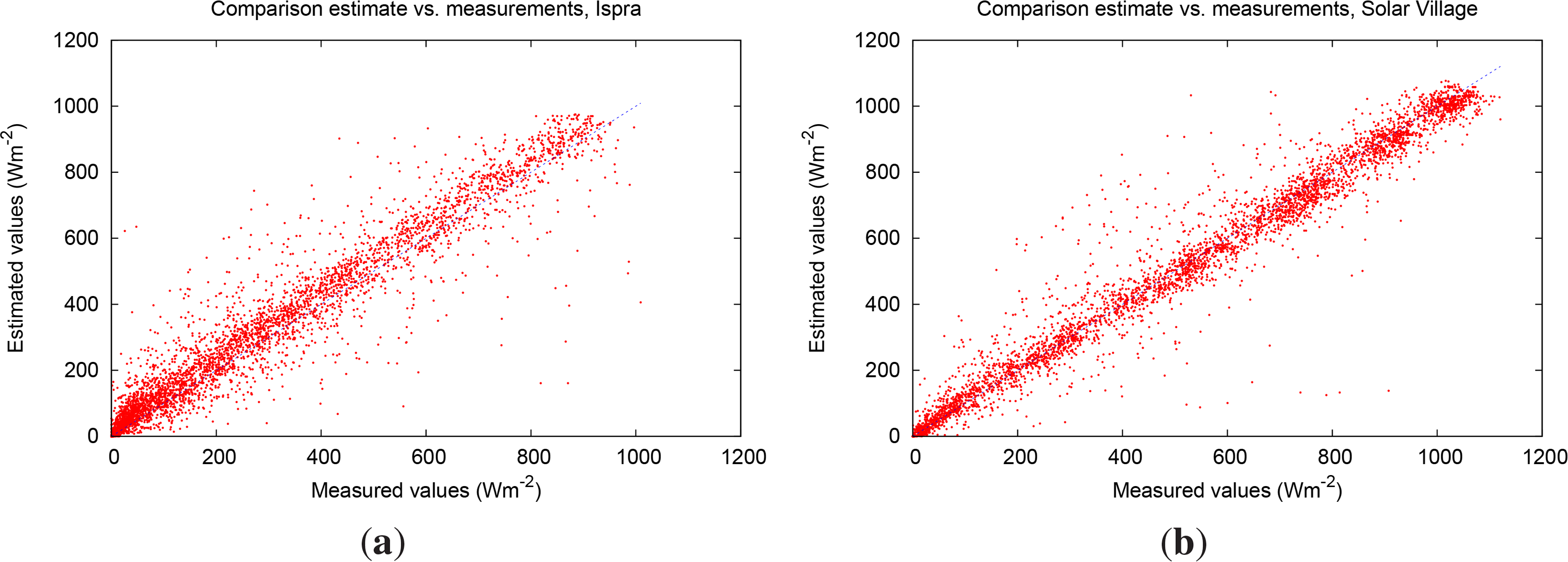
A graphical comparison of the measured and estimated values is shown in Figure 1, for two stations: Solar Village in a desert climate and Ispra, Italy which is a humid temperate climate. The overall MBD for Solar Village is very low, while the Ispra location has the highest MBD of all stations. The pattern of results is rather different for the two stations. For Solar Village, the majority of points are below the diagonal (estimated is lower than measured), with a number of scattered points far above the diagonal. This is consistent with the finding that the estimates tend to be too low for clear-sky conditions and too high for more cloudy conditions. For Ispra, the estimated values are generally higher than measurements at all irradiance levels. This could be due to an underestimate of the effects of aerosols. It might also indicate a problem in the measurements.
As mentioned in the beginning of this section, all the validation data are available online. The interested reader may use these data to produce similar plots for any of the stations used in the validation exercise.
3.4. Validation Results, Direct Normal Irradiance
The algorithm described in Section 2.1 can also estimate the direct component of the solar radiation, either as direct horizontal or direct normal irradiance. DNI is also measured at nearly all BSRN stations as well as at some of the non-BSRN stations used for the validation in the previous section.
Table 5 shows the results of the validation of DNI estimates from the SPECMAGIC model, using the stations that have DNI data available.
The relative global mean absolute bias (rgMAB) and relative global root mean square deviation (rgRMSD) have values rgMAB = 5.03% and rgRMSD = 6.30%. These values are significantly higher than the corresponding values for the global horizontal irradiance.
For most stations, the mean bias deviation value is higher than the one observed in the validation of the global irradiance. Also, the rMAB and rRMSD values are approximately twice as high as those of the global irradiance. However, when global statistics are analyzed we can see that the global MBD for all the stations and the relative global MBD are lower in the validation of the beam component than for the global irradiance. The higher deviations of the estimated beam irradiance, in some cases as overestimation and in other as underestimation, tend to compensate better than in the case of the global irradiance. The very low overall MBD for DNI should therefore be regarded as fortuitous.
As for the global irradiance estimates, we can calculate the global statistical quantities in Equations (A7)–(A9). The average measured DNI of all the stations is DNIavg = 214.62 Wm−2, and the global mean bias deviation is gMBD = 0.61 Wm−2. The relative global bias is rgMBD = 0.62%.
3.5. Comparison of Irradiance Probability Density
Besides the statistical measures (MBD, MAB, RMSD, etc.) used for the validation of the estimation model, it is interesting to analyze the probability distribution of the irradiance values, to see if the occurrence of the different irradiance levels are properly represented by the model.
For this analysis, the data when the sun’s elevation angle is below 5 degrees are not considered. The remaining data are distributed into bins of width 50 Wm−2 from 0 to 1200 Wm−2. For the direct irradiance the 0Wm−2 value will not be displayed, in order to avoid the high peak in the probability distribution at that level of irradiance.
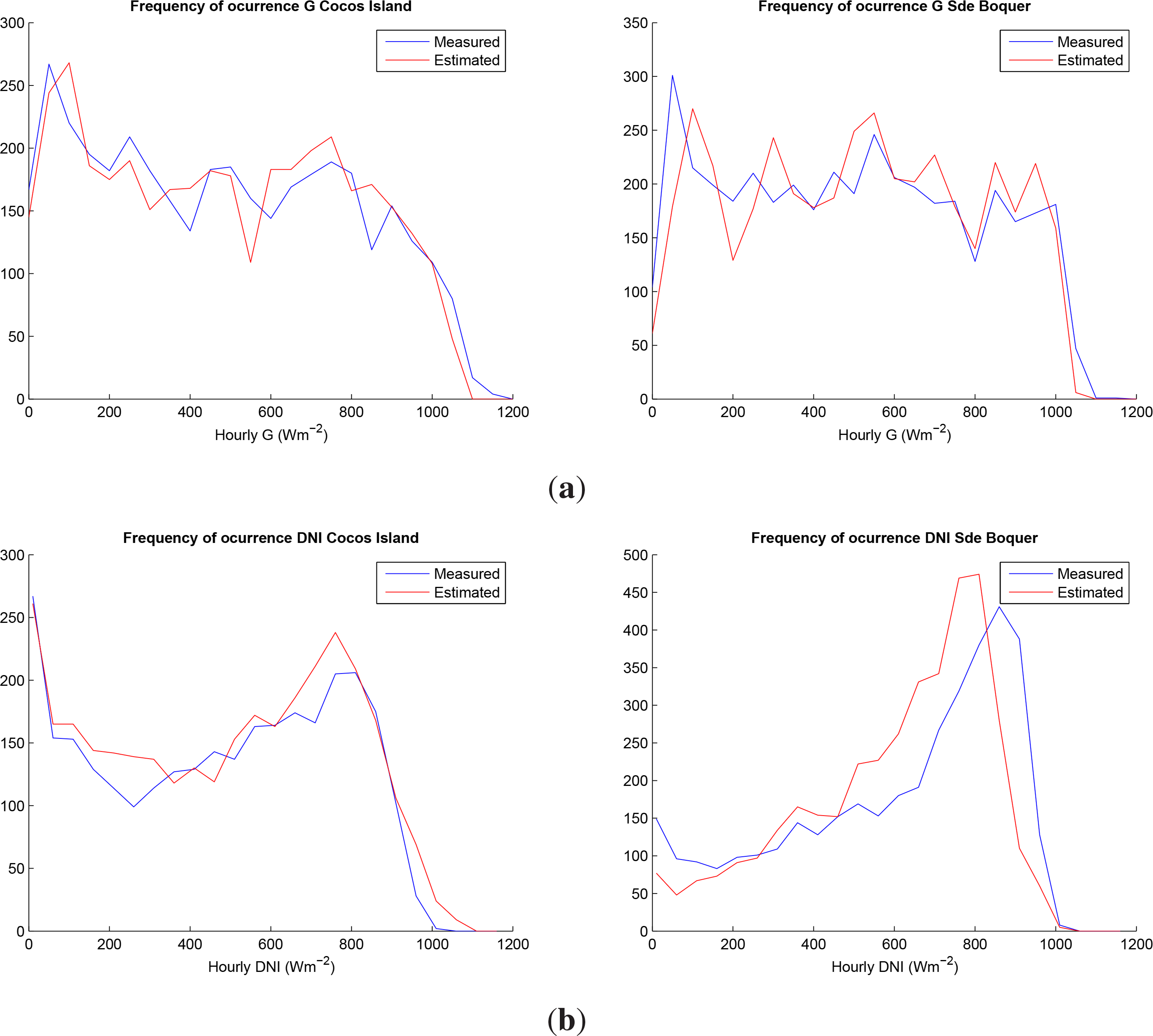
As an example of the probability distribution graphs, those of the global and direct normal irradiances for Cocos Island and Sde Boqer are shown in Figure 2. These two stations have been chosen as they represent quite different climates.
For the global irradiance, in general, the model does not provide the very low and high irradiance values measured at the stations. For intermediate irradiance levels, there is no clear pattern. For the two stations shown in Figure 2, the overestimation derived from the model for Sde Boqer (+8.41 Wm−2) is reflected in the graph where it is seen that the model has too many occurrences at high irradiance (800–900 Wm−2) and too few at low irradiance (<100 Wm−2). For Cocos Island there are no consistent differences in the intermediate irradiance range.
Regarding the frequency distribution of the beam normal irradiance values, the general trend for the various stations is the one observed in Sde Boqer. There is a higher number of observations of very high irradiance values that are not reached by the estimation model, while for the intermediate irradiance levels, the estimated values show a higher occurrence. However, it is the opposite case in Cocos Island, especially in the range of high beam irradiance values. This is reflected in the overall high positive bias (+22.94 Wm−2). This is likely to be due to an underestimation of the aerosol content in the area, leading to an overestimate of DNI under clear-sky conditions.
The lack of very high DNI values in the satellite estimates may be due to the fact that we are using long-term averages of AOD data. Periods with exceptionally low aerosol load will tend to have very high DNI values, which will be seen in the measurements but not captured by the satellite-based estimates.
The hourly estimated and measured data are available in the online supplementary material. This allows interested readers to construct these graphs for any station in the validation data set.
4. Results and Discussion
The methods described in Section 2 have been used to calculate solar radiation parameters for every full-hour time slot in the period 1999–2013, with a hiatus in 2006 due to uncertainty about the quality of data from Meteosat-5 towards the end of the operational life of that satellite. Thus, a total of 14 years are available, which makes it possible to calculate long-term averages with low uncertainty from interannual variation.
4.1. Sample Results
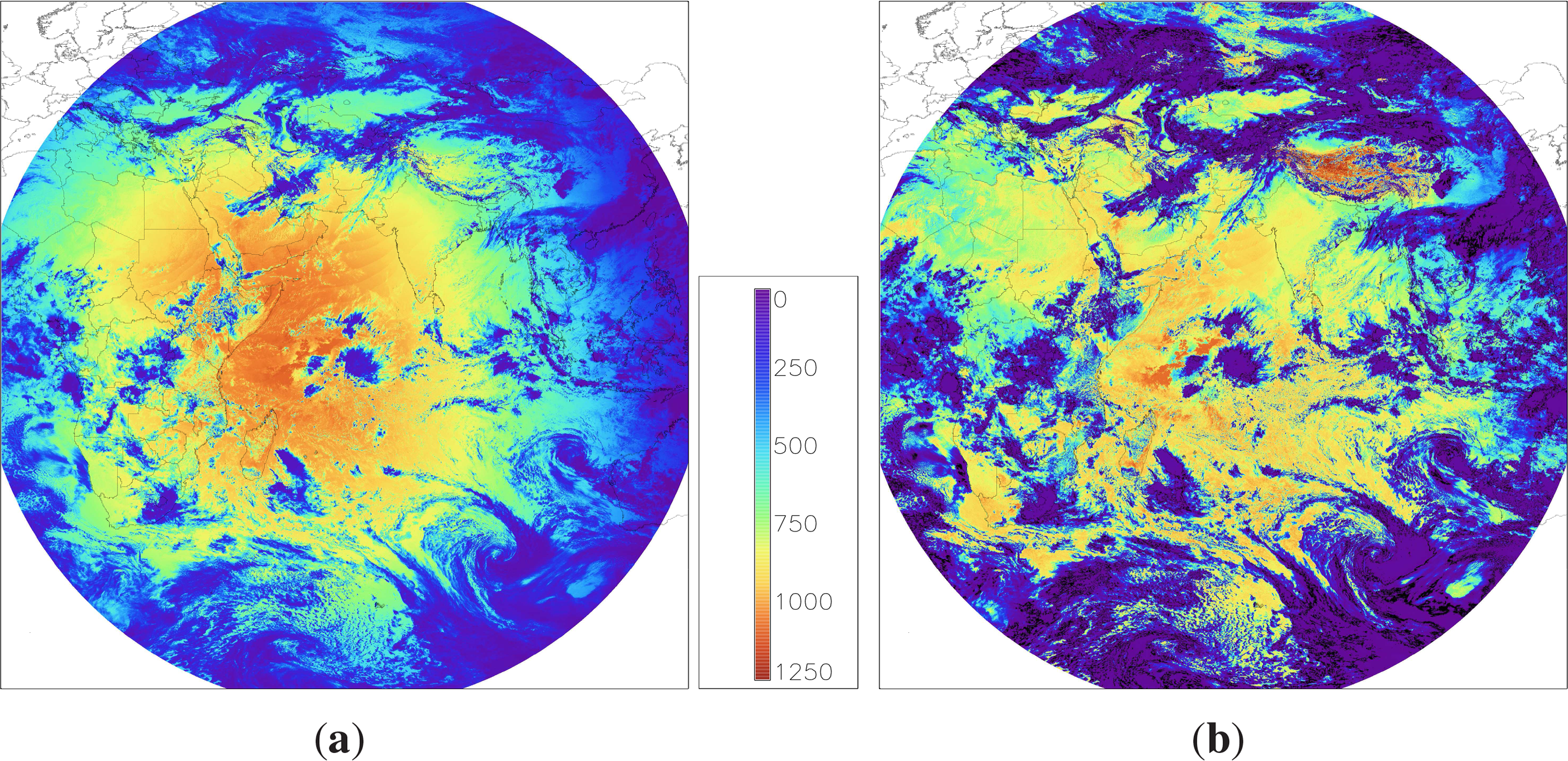
An example of a map of solar irradiance (global horizontal and direct normal) is shown in Figure 3. The time slot is 09:00GMT on 14 March 2005, showing the maximum irradiance, corresponding to cloudless conditions, just west of the center of the image (which is at 63°E), and illustrating the overall extent of valid data.
4.2. Comparison of Meteosat Prime and East Estimates
From 1998 to 2006 two very similar satellites were both in orbit at the same time at widely different positions (Meteosat 7 at 0° and Meteosat 5 at 63°E). This makes it possible to do a direct comparison of the solar radiation retrieval from the two satellites in the area where they overlap.
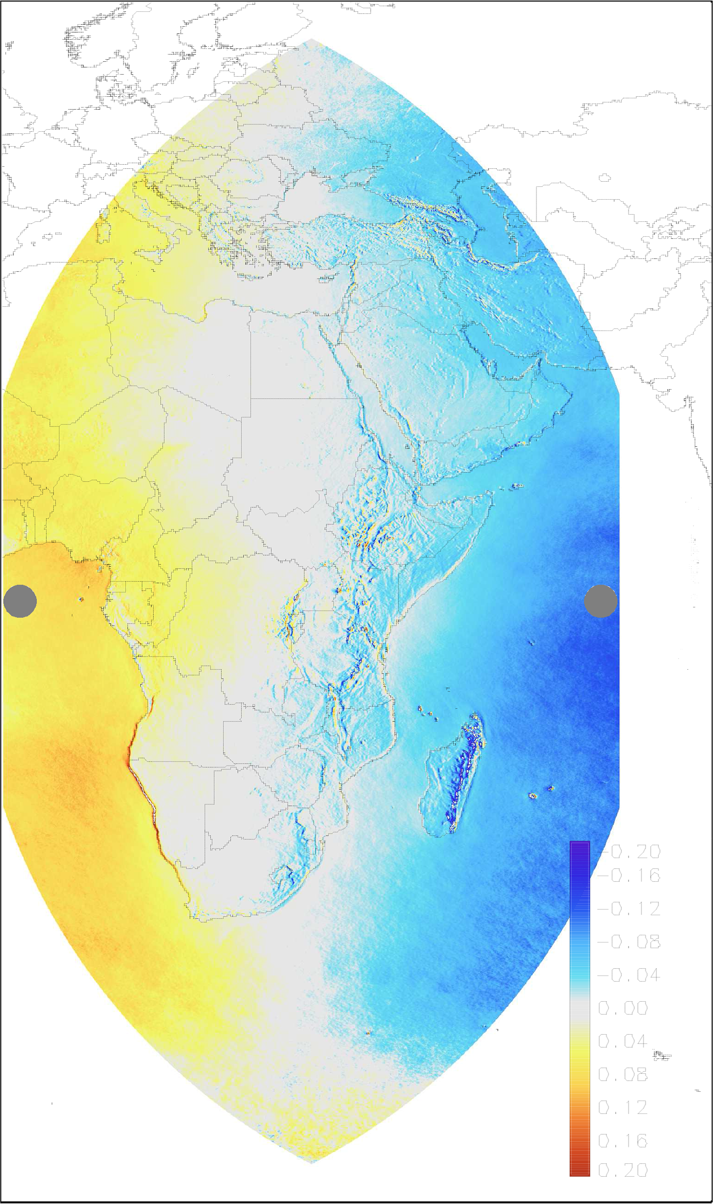
Figure 5 shows a map of the relative difference between H for the year 2005 calculated from the two satellites, defined as:
The result shows a significant gradient in the east-west direction, with estimates from Meteosat Prime higher than those of Meteosat East in the western part and vice versa in the eastern part. This means that the retrieval algorithm tends to give lower values near the edge of the satellite image.
The effects of aerosols and water vapour are calculated by the clear-sky radiation model and are therefore independent of the viewing angle of the satellite, so the differences shown in Figure 5 must in some way be due to the effect of clouds, either in the calculation of CAL or in the treatment of clouds by the SPECMAGIC algorithm. A possible explanation is that due to the finite thickness of clouds, broken cloud fields can be identified when viewed directly from above (close to the satellite nadir) but will appear as continuous cloud cover when viewed from a shallow angle (as is the case near the edge of the image). This would lead to an overestimation of cloudiness and hence an underestimation of radiation.
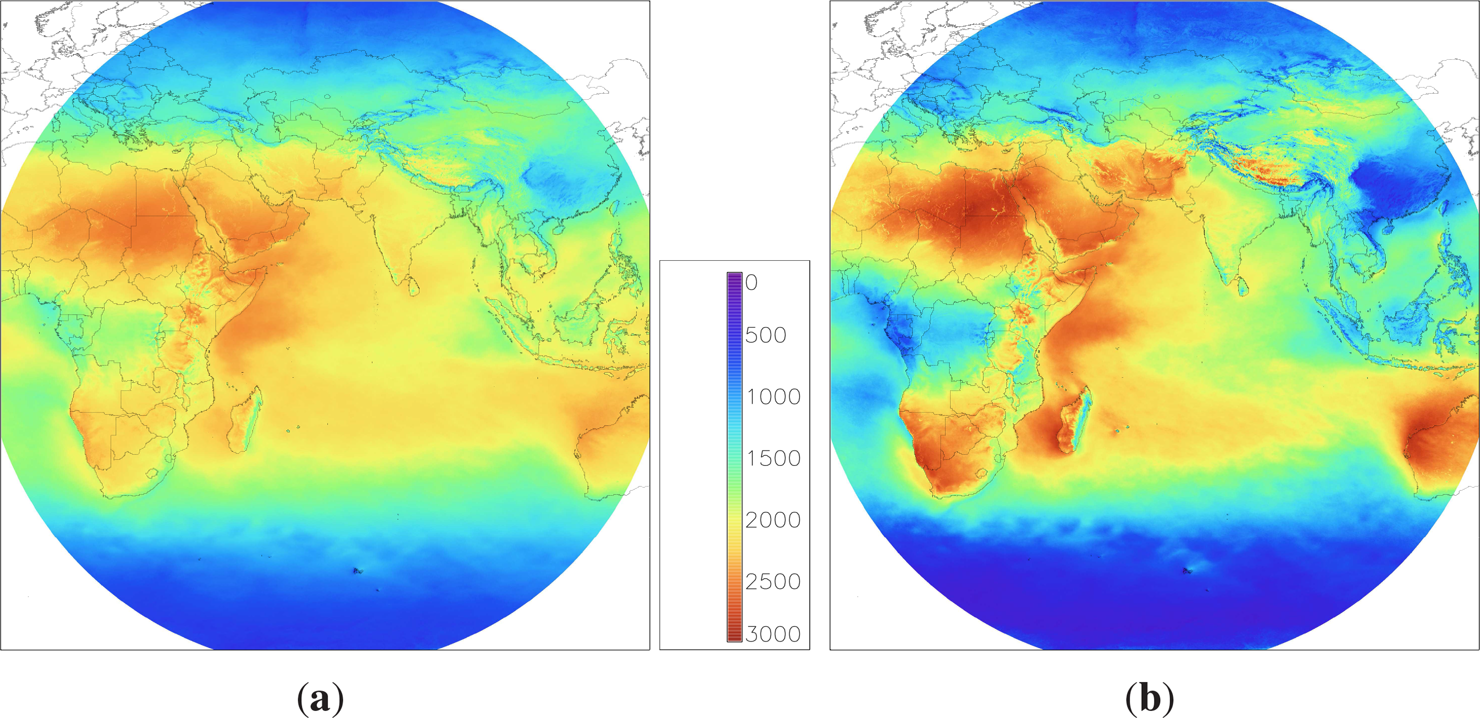
The individual hourly slots can be summed to produce maps of the global horizontal and direct normal irradiation for longer time periods. Figure 4 shows H and HDNI for the year 2002.
In the validation results shown in Table 3 some of the stations were visible from both satellites at the same time. For these stations the same trend is seen. De Aar and Thessaloniki are both closer in longitude to the Meteosat Prime nadir, and their MBD is more positive for Meteosat Prime (at De Aar, rMBD is 0.60% for Meteosat Prime vs. −1.21% for Meteoast East, while for Thessaloniki the values are +3.55% vs. −3.64%). Solar Village is closer to Meteosat East and has rMBD of −2.55% for Meteosat Prime and −0.23% for Meteosat East. Sde Boqer and Kishinev are close being at equal distance to the two satellites, and here we see rather little difference in rMBD (3.41% vs. 3.94% for Sde Boqer, 1.37% vs. 0.50% for Kishinev).
An analogous case is evident in mountain areas which often have very localized gradients in the available solar radiation. In some cases the local patterns are shifted relative to each other in the data sets obtained from the two different satellites. This may be due to the effect of parallax when the two satellites are observing persistent cloud systems over mountains from different angles. This effect will lead to an increased uncertainty in mountainous regions.
4.3. Comparing the Results with Existing Databases
In the scientific bibliography there are several publications in which solar radiation estimates retrieved from satellite images are validated by comparison with ground measurements. The validation is commonly performed on daily or monthly average irradiance values, although in some cases hourly irradiance values are analyzed, like in this paper.
Two examples of hourly validation data were performed by Ineichen (2011 and 2013) [35,36]. The author compared the irradiance values derived from various satellite products with the measurements registered in several stations. It should be noted that these data sets are derived from the Meteosat MSG class of satellites, so the methods employed are somewhat different. Nevertheless it is possible to get an idea of how the accuracy of the present data set compares with other recent efforts.
A detailed description of the method we used to compare these results is found in the supplementary material [28].
Data of global horizontal and beam normal irradiance are validated in hourly values. The magnitude of the errors is similar of those reported in this paper.
In the first report [35], five different satellite products are validated: SolarGis, Helioclim 3 data bank, 3Tier algorithm, EnMetSol considering two different clear sky models (denoted Solis and Dumortier) and IrSolAv estimates. The estimates are validated with irradiance measurements registered at 20 stations in the case of the global horizontal irradiance and 12 stations for the beam component. The validation results for G and DNI are shown in Table 6.
The magnitude of the general statistics are similar to those obtained in the present paper. The validation of the SPECMAGIC estimates reports rgMBD, rgMAB and rgRMSD values as low as the best satellite product analyzed in [35], for both G and DNI.
If the validation of the global irradiance on the horizontal plane is performed distributing the data according to sky type, we obtain the results shown in Table 7. Again, the results are similar to those derived from the SPECMAGIC method.
For all satellite products considered, including SPECMAGIC estimates, the global horizontal irradiance is underestimated in clear sky situations, while for intermediate and more significantly overcast situations, the solar resource is overestimated.
It should be noted that although the number of stations used in [35] is similar to that used in the present study, there is not a great overlap in the actual list of stations. In fact, only 8 stations used in [35] are the same as those we have used. This may skew the results because some station locations may be more “challenging” than others for the algorithms. We have therefore repeated the comparison using these 8 stations: Cabauw, Camborne, Carpentras, Payerne, Sde Boqer, Thessaloniki, Toravere (Thessaloniki is used for the DNI comparison). IrSolAv was not validated for all these stations and therefore has been excluded from this comparison. These results are given in Table 8.
Given the low number of stations, it is difficult to clearly distinguish between the values for the different products. It is possible to do a test for statistical significance of the differences in the global variances (the square of rgRMSD). A two-tailed f-test statistic (7times7 degrees of freedom) on the values for G in Table 8 shows that only SolarGIS is significantly better than the results from SPECMAGIC (p < 0.04). For the DNI comparison (7 stations), none of the rgRMSD results from [35] are significantly different from the SPECMAGIC result.
Similarly, for the results in Table 6, few of the differences in rgRMSD between SPECMAGIC and the other products are statistically significant: only the differences with Heliosat 3 (G and DNI) and 3Tier (DNI) are statistically significant at p < 0.05. As noted previously, this may be in part due to the difference in choice of stations.
In the second report [36], six different satellite products are validated: SolarGis, Helioclim 3, Solemi, Heliomont (Meteoswiss), EnMetSol, IrSolAv. Estimates are compared with global horizontal and beam normal irradiance experimental data registered at 17 stations. Results are shown in Table 9. Again, the range of the statistics is similar to that observed in the present work. In this case, the number of stations in common is even smaller, and a comparison for these few stations does not make statistical sense.
5. Conclusions
We have presented the results of applying the Heliosat and SPECMAGIC algorithms to images from the Meteosat Eastern geostationary satellites in order to produce hourly maps of surface solar irradiance (global and direct). For validation purposes, estimates from the Meteosat Prime satellites were also produced. Validation from 16 ground stations show a low overall yearly bias (gMBD) in the estimation of the global horizontal irradiance of +1.63 Wm−2 or +0.73%. The mean absolute bias of the individual station bias values (rgMAB) is 2.36% while the root-mean-square of the station bias values (rgRMSD) is 3.18%. For the annual average DNI estimation, the corresponding values are: gMBD = +0.61 Wm−2 or +0.62%, rgMAB = 5.03%, and rgRMSD = 6.30%. The very low gMBD value is a fortuitous cancelling of individual deviations. The two latter values give a better idea of the uncertainty in estimates at individual locations. A comparison with validation results given by Ineichen [35,36] shows that the accuracy of the present results is similar to that of other recent works on satellite-based solar radiation databases.
The overall deviations from measured data are quite low. However, there are still areas where improvements could be made. A direct comparison between solar radiation estimates from the Meteosat Prime and East over the same time period shows that the radiation estimates tend to be higher near the center of the satellite image than near the edge. This is probably due to the fact that the finite thickness of clouds will make the cloud cover seem more extensive when viewed at a shallow angle as is the case near the edge of the satellite image. To resolve this issue would require more information about cloud type than is currently available in the method.
For the time being, there is no particular treatment of snow cover in the method, so areas affected by snow may have larger uncertainties. Since none of the validation stations are in high mountain or arctic areas, this problem is not seen in the validation results but should be acknowledged anyway. Methods to account for snow cover are being studied at present and will be applied to future versions of the solar radiation database.
For the present study, long-term monthly averages of aerosol data have been employed, as described in Section 2.2. This choice may have an influence on the year-to-year variability of the total solar radiation, which is of interest to investors and operators of solar energy power plants. We plan to investigate the influence of using monthly aerosol data on the resulting solar radiation time series.
Once processing has been completed, the hourly maps of solar radiation will be made freely available to the public. To our knowledge, this new data set is the first freely available high-resolution solar radiation data set covering Asia (there exist several for Europe and Africa, and free data are to some extent also available for the Americas). The new data set should be useful for researchers, planners and installers of solar energy systems, as well as for studies of climate and biological processes.
The SPECMAGIC method can also calculate spectrally resolved solar irradiance. We plan to use this feature to produce maps of spectrally resolved irradiance to study the effects of spectral changes on PV system productivity for the area covered by the data. Maps of photosynthetically active radiation may also be produced.
Solar radiation data are essential for the estimation of solar energy system performance. An important application of the data presented in this study will be to perform estimates of solar energy system performance. In particular, it is planned that these data will be incorporated into the web-based PV estimation tool PVGIS [37,38].
Nomenclature
| Acronyms | |
|---|---|
| BSRN | Baseline Surface Radiation Network |
| CM SAF | Climate Monitoring Satellite Application Facility |
| DNI | Direct Normal Irradiance |
| ECMWF | European Centre for Medium-range Weather forecast |
| GAW | Global Atmosphere Watch |
| MACC | Monitoring Atmospheric Composition and Climate |
| MFG | Meteosat First Generation satellites |
| MSG | Meteosat Second Generation satellites |
| NWP | Numerical Weather Prediction |
| PV | Photo-Voltaic |
| PVGIS | PhotoVoltaic Geographical Information System |
| RTM | Radiative Transfer Model |
| SAL | Surface ALbedo |
| USGS | United States Geological Survey |
| Symbols | |
|---|---|
| AM | Air Mass (-) |
| B, Bclear, Ball | Direct (beam) radiation, clear-sky & all-sky beam radiation (Wm−2) |
| CAL | Effective Cloud Albedo, also called Cloud Index (-) |
| D | Digital count of the satellite instrument |
| DNI, DNIavg | Direct normal irradiance & average DNI of all stations (Wm−2) |
| G | Global horizontal irradiance (Wm−2) |
| Gavg | Average measured irradiance of all the stations (Wm−2) |
| Gmeas | Measured Global horizontal irradiance (Wm−2) |
| Gclear | Global horizontal clear-sky irradiance (Wm−2) |
| H | Global horizontal irradiation (kWh m−2) |
| HDNI | Direct normal irradiation (kWh m−2) |
| ΔH | Relative difference in H between the two satellites (%) |
| kc | Clear-sky index (-) |
| kt | Clearness index (-) |
| k′t | Modified clearness index (-) |
| MAB, rMAB | Mean Absolute Bias, relative Mean Absolute Bias |
| gMAB, rgMAB | global Mean Absolute Bias, relative global Mean Absolute Bias |
| MBD, rMBD | Mean Bias Deviation, relative Mean Bias Deviation |
| gMBD, rgMBD | global Mean Bias Deviation, relative global Mean Bias Deviation |
| N | Number of data points used for the validation (-) |
| Ns | Number of ground stations used for the validation (-) |
| ρ | Intensity of reflected light measured by satellite (-) |
| ρthres | Threshold value of ρ, for calibration of satellite measurements (-) |
| ρcs, ρmax | Clear-sky and monthly maximum values of ρ (-) |
| ρmax,corr | Value of ρmax corrected as a function of θ (-) |
| RMSD, rRMSD | Root Mean Square Deviation, relative Root Mean Square Deviation |
| gRMSD, rgRMSD | global Root Mean Square Deviation, relative global Root Mean Square Deviation |
| θ | Solar zenith angle (-) |
| Subscript i | i’th time series value |
| Superscript m | measured value |
| Superscript r | retrieved (estimated) value |
Acknowledgments
We would like to thank EUMETSAT for the access to satellite image data and the CM SAF Project for the possibility to use the algorithms developed within that project.
Author Contributions
The contributions of each author to the work described in this paper are as follows:
Ana Gracia Amillo did most of the work on validation of satellite data against ground station data and the comparison with other recent work and wrote the section on validation and parts of the results & discussion.
Thomas Huld performed the data processing for Meteosat East and some of the Meteosat Prime data, as well as postprocessing to produce annual means and differences between satellites (Figures 3 and 5). He wrote most of the introduction and conclusions and part of the discussion.
Richard Müller produced an updated version of the SPECMAGIC code and processed the climatological data needed as input. He wrote most of the section on methods.
Conflicts of Interest
The authors declare no conflict of interest.
Appendix Statistical Measures Used for the Validation
A number of different statistical measures have been used to estimate the uncertainty in the irradiance retrieved from satellite data. These are defined briefly here.
For a given set of data (station or satellite-based estimate), the annual average is calculated from the N values:
The Mean Bias Deviation (MBD) is calculated as shown in Equation (A2):
Here is the measured irradiance at the ith time point while is the estimated irradiance at the same time point. In this calculation both day and night time slots are considered. N is the total number of time points for which both measured and estimated data are available.
The relative MBD (rMBD) is defined in Equation (A3) as:
The Mean Absolute Bias (MAB) is calculated as (Equation (A4)):
The Root Mean Square Deviation (RMSD) is given as:
Relative values of MAB and RMSD are calculated like Equation (A3): rMAB = MAB/〈G〉 and rRMSD = RMSD/〈G〉
To get an overall estimate of the bias in yearly average solar irradiation, we can calculate the avarage of the MBD values at all the station locations. This is termed the global MBD (and respectively, relative global MBD):
Here, MBDs is the MBD of station number s. Ns is the number of stations.
A measure of the uncertainty of the yearly average irradiation in a given point can be given as the relative global MAB and RMSD:
References
- Möser, W.; Raschke, E. Incident solar radiation over europe estimated from METEOSAT data. J. Clim. Appl. Meteor 1984, 23, 166–170. [Google Scholar]
- Cano, D.; Monget, J.; Albuisson, M.; Guillard, H.; Regas, N.; Wald, L. A method for the determination of the global solar radiation from meteorological satellite data. Solar Energy 1986, 37, 31–39. [Google Scholar]
- Pinker, R.; Laszlo, I. Modelling surface solar irradiance for satellite applisations on a global scale. J. Appl. Meteorol 1992, 31, 166–170. [Google Scholar]
- Meyer, R.; Hoyer, C.; Schillings, C.; Trieb, F.; Diedrich, E.; Schroedter, M. SOLEMI: A new satellite-based service for high-resolution and precision solar radiation data for Europe, Africa and Asia. Proceedings of the 2003 ISES Solar World Congress, GÃűteborg, Sweden, 14–19 June 2003.
- Müller, R.; Matsoukas, C.; Gratzki, A.; Behr, H.; Hollmann, R. The CM-SAF operational scheme for the satellite based retrieval of solar surface irradiance—A LUT based eigenvector hybrid approach. Remote Sens. Environ 2009, 113, 1012–1024. [Google Scholar]
- Rigollier, C.; Levefre, M.; Wald, L. The method Heliosat-2 for deriving shortwave solar radiation from satellite images. Solar Energy 2004, 77, 159–169. [Google Scholar]
- Laszlo, I.; Ciren, P.; Liu, H.; Kondragunta, S.; Tarpley, J.D.; Goldberg, M.D. Remote sensing of aerosol and radiation from geostationary satellites. Adv. Space Res 2008, 41, 1882–1893. [Google Scholar]
- Karlsson, K.-G.; Riihelä, A.; Müller, R.; Meirink, J.F.; Sedlar, J.; Stengel, M.; Lockhoff, M.; Trentmann, J.; Kaspar, F.; Hollmann, R.; et al. CLARA-A1: The CM SAF cloud, albedo and radiation dataset from 28 yr of global AVHRR data. Atmos. Chem. Phys. Discuss 2013, 13, 935–982. [Google Scholar]
- SOLEMI. Available Online: http://www.dlr.de/tt/solemi (accessed on 26 August 2014).
- Blanc, P.; Gschwind, B.; Lefèvre, M.; Wald, L. The HelioClim project: Surface solar irradiance data for climate applications. Remote Sens 2011, 3, 343–361. [Google Scholar] [CrossRef]
- CM SAF. Available Online: http://www.cmsaf.eu (accessed on 26 August 2014).
- Geiger, B.; C. Meurey, D.; Lajas, L.; Franchistéguy, L.; Carrer, D.; Roujean, J.-L. Near real-time provision of downwelling shortwave radiation estimates derived from satellite observations. Meteorol. Appl 2008, 15, 411–420. [Google Scholar]
- LSA SAF. Available Online: http://landsaf.meteo.pt (accessed on 26 August 2014).
- Müller, R.; Behrendt, T.; Hammer, A.; Kemper, A. A new algorithm for the satellite-based retrieval of solar surface irradiance in spectral bands. Remote Sens 2012, 4, 622–647. [Google Scholar]
- Müller, R.; Trentmann, J.; Träger-Chatterjee, C.; Posselt, R.; Stöckli, R. The Role of the Effective Cloud Albedo for Climate Monitoring and Analysis. Remote Sens 2011, 3, 2305–2320. [Google Scholar]
- Hammer, A.; Heinemann, D.; Hoyer, C.; Kuhlemann, R.; Lorenz, E.; Müller, R.; Beyer, H. Solar energy assessment using remote sensing technologies. Remote Sens. Environ 2003, 86, 423–432. [Google Scholar]
- Posselt, R.; Müller, R.; Stöckli, R.; Trentmann, J. Spatial and temporal homogeneity of solar surface irradiance across satellite generations. Remote Sens 2011, 3, 1029–1046. [Google Scholar]
- Skartveit, A.; Olseth, J.; Tuft, M. An hourly diffuse fraction model with correction for variability and surface albedo. Solar Energy 1998, 63, 173–183. [Google Scholar]
- Dee, D.P.; Uppala, S.M.; Simmons, A.J.; Berrisford, P.; Poli, P.; Kobayashi, S.; Andrae, U.; Balmaseda, M.A.; Balsamo, G.; Bauer, P.; et al. The ERA-Interim reanalysis: Configuration and performance of the data assimilation system. Q. J. R. Meteorol. Soc 2011, 137, 553–597. [Google Scholar]
- ECMWF. Available Online: http://www.ecmwf.int (accessed on 26 August 2014).
- Morcrette, J.-J.; Boucher, O.; Jones, L.; Salmond, D.; Bechtold, P.; Beljaars, A.; Benedetti, A.; Bonet, A.; Kaiser, J.W.; Razinger, M.; et al. Aerosol analysis and forecast in the European Centre for Medium-Range Weather Forecasts Integrated Forecast System: Forward modeling. J. Geophys. Res 2009, 114. [Google Scholar] [CrossRef]
- Benedetti, A.; Morcrette, J.-J.; Boucher, O.; Dethof, A.; Engelen, R.J.; Fisher, M.; Flentje, H.; Huneeus, N.; Jones, L.; Kaiser, J.W.; et al. Aerosol analysis and forecast in the European Centre for Medium-Range Weather Forecasts Integrated Forecast System: 2. Data assimilation. J. Geophys. Res 2009, 114. [Google Scholar] [CrossRef]
- Inness, A.; Baier, F.; Benedetti, A.; Bouarar, I.; Chabrillat, S.; Clark, H.; Clerbaux, C.; Coheur, P.; Engelen, R.J.; Errera, Q.; et al. TheMACC reanalysis: An 8 yr data set of atmospheric composition. Atmos. Chem. Phys 2013, 13, 4073–4109. [Google Scholar]
- MACC. Available Online: http://www.gmes-atmosphere.eu (accessed on 26 August 2014).
- Brown, J.F.; Loveland, T.; Merchant, J.W.; Reed, B.C.; Ohlen, D.O. Using multi-source data in global land-cover characterization: Concepts, requirements, and methods. Photogramm. Eng. Remote Sens 1983, 59, 977–987. [Google Scholar]
- Dickinson, R.E. Land surface processes and climate—Surface albedos and energy balance. Adv. Geophys 1983, 25, 305–353. [Google Scholar]
- EUMETSAT. Available Online: http://www.eumetsat.int (accessed on 26 August 2014).
- A New Database of Global and Direct Solar Radiation Using the Eastern Meteosat Satellite,Models and Validation. Available Online: http://re.jrc.ec.europa.eu/esti/meteast/index.html (accessed on 26 August 2014).
- Baseline Surface Radiation Network. Available Online: http://bsrn.awi.de (accessed on 26 August 2014).
- Global Atmosphere Watch. Available Online: http://www.wmo.int/gaw/ (accessed on 26 August 2014).
- World Radiation Data Centre. Available Online: http://wrdc.mgo.rssi.ru (accessed on 26 August 2014).
- Ineichen, P.; Barroso, C.S.; Geiger, B.; Hollmann, R.; Marsouin, A.; Müller, R. Satellite Application Facilities irradiance products: Hourly time step comparison and validation over Europe. Int. J. Remote Sens 2009, 30, 5549–5571. [Google Scholar]
- Perez, R.; Ineichen, P.; Seals, R.; Zelenka, A. Making full use of the clearness index for parametrizing hourly insolation conditions. Solar Energy 1990, 45, 111–114. [Google Scholar]
- Kasten, F. A simple parameterization of two pyrheliometric formulae for determining the Linke turbidity factor. Meteorol. Rdsch 1980, 33, 124–127. [Google Scholar]
- Ineichen, P. Five Satellite Products Deriving Beam and Global Irradiance Validation on Data from 23 Ground Stations. Available online: http://archive-ouverte.unige.ch/unige:23669 (accessed on 26 August 2014).
- Ineichen, P. Long Term Satellite Hourly, Daily and Monthly Global, Beam and Diffuse Irradiance Validation. Interannual Variability Analysis. Available online: http://archive-ouverte.unige.ch/unige:29606 (accessed on 26 August 2014).
- Huld, T.; Müller, R.; Gambardella, A. A new solar radiation database for estimating PV performance in Europe and Africa. Solar Energy 2012, 86, 1803–1815. [Google Scholar]
- PVGIS. Available Online: http://re.jrc.ec.europa.eu/pvgis/ (accessed on 26 August 2014).


| Satellite | Class | Start Date | End Date | Longitude |
|---|---|---|---|---|
| Meteosat-5 | MFG | 2 May 1991 | 13 February 1997 | 0° |
| Meteosat-5 | MFG | 1 July 1998 | 16 April 2007 | 63°E |
| Meteosat-7 | MFG | 6 March 1998 | 19 July 2006 | 0° |
| Meteosat-7 | MFG | 1 November 2006 | ongoing | 57°E |
| Station | Lat | Lon | Climate type | Prime | East | Years Used |
|---|---|---|---|---|---|---|
| BSRN stations | ||||||
| Cabauw (NL) | 51.97N | 4.93E | Temperate maritime | X | 2005 | |
| Camborne (UK) | 50.22N | 5.32W | Temperate maritime | X | 2005 | |
| Carpentras (FR) | 44.05N | 5.03E | Mediterranean | X | 2005 | |
| Cocos Island (AU) | 12.19S | 96.84E | Tropical wet | X | 2009 | |
| De Aar (ZA) | 30.67S | 23.99E | Arid | X | X | 2002 |
| Florianopolis (BR) | 27.53S | 48.52W | Humid subtropical | X | 2005 | |
| Lindenberg (DE) | 52.22N | 14.12E | Moderate maritime | X | 2005 | |
| Payerne (CH) | 46.81N | 6.94E | Semi continental | X | 2005 | |
| Sde Boqer (IL) | 30.87N | 34.77E | Dry steppe | X | X | 2005, 2009 |
| Solar Village (SA) | 24.91N | 46.78E | Arid | X | X | 2002 |
| Tamanrasset (DZ) | 22.79N | 5.53E | Hot, desert | X | 2005 | |
| Toravere (EE) | 58.27N | 26.47E | Cold humid | X | 2005 | |
| Xianghe (CN) | 39.75N | 116.96E | Continental humid | X | 2005 | |
| Non-BSRN stations | ||||||
| Ispra (IT) | 45.81N | 8.63E | Mediterranean moist | X | 2005 | |
| Kishinev (MD) | 47.00N | 28.82E | Cool temperature, moist | X | X | 2005 |
| Thessaloniki (GR) | 40.63N | 22.96E | Mediterranean temperate | X | X | 2005 |
| Station | Year | (Gmeas) Wm−2 | MBD (Wm−2) | rMBD (%) | MAB (Wm−2) | rMAB (%) | RMSD (Wm−2) | rRMSD (%) |
|---|---|---|---|---|---|---|---|---|
| Meteosat PRIME | ||||||||
| De Aar | 2002 | 257 | 1.54 | 0.60 | 27.42 | 10.67 | 66.13 | 25.73 |
| Solar Village | 2002 | 280 | −7.16 | −2.55 | 22.22 | 7.93 | 48.11 | 17.17 |
| Cabauw | 2005 | 137 | −0.50 | −0.37 | 28.31 | 20.68 | 62.19 | 45.44 |
| Camborne | 2005 | 130 | −2.40 | −1.85 | 26.85 | 20.71 | 58.26 | 44.93 |
| Carpentras | 2005 | 185 | 10.10 | 5.47 | 22.85 | 12.38 | 52.75 | 28.57 |
| Florianopolis | 2005 | 188 | 0.54 | 0.29 | 39.63 | 21.13 | 89.54 | 47.73 |
| Ispra | 2005 | 154 | 13.85 | 9.02 | 27.41 | 17.85 | 58.65 | 38.20 |
| Kishinev | 2005 | 149 | 2.05 | 1.37 | 30.78 | 20.59 | 61.89 | 41.40 |
| Lindenberg | 2005 | 133 | −4.29 | −3.22 | 27.26 | 20.49 | 62.59 | 47.04 |
| Payerne | 2005 | 151 | 0.89 | 0.58 | 29.69 | 19.61 | 64.49 | 42.60 |
| Sde Boqer | 2005 | 250 | 8.53 | 3.41 | 23.76 | 9.94 | 53.00 | 21.18 |
| Tamanrasset | 2005 | 266 | 6.98 | 2.63 | 26.56 | 10.00 | 64.96 | 24.45 |
| Thessaloniki | 2005 | 194 | 6.90 | 3.55 | 31.55 | 16.22 | 61.23 | 31.49 |
| Toravere | 2005 | 119 | −4.94 | −4.14 | 27.43 | 23.00 | 60.90 | 51.07 |
| Meteosat EAST | ||||||||
| De Aar | 2002 | 250 | −3.02 | −1.21 | 28.91 | 11.55 | 71.32 | 28.50 |
| Solar Village | 2002 | 273 | −0.62 | −0.23 | 20.50 | 7.51 | 48.92 | 17.91 |
| Kishinev | 2005 | 151 | 0.75 | 0.50 | 32.62 | 21.64 | 64.76 | 42.97 |
| Sde Boqer | 2005 | 251 | 9.89 | 3.94 | 27.25 | 10.84 | 60.07 | 23.90 |
| Thessaloniki | 2005 | 194 | −7.05 | −3.64 | 40.14 | 20.70 | 79.40 | 40.95 |
| Xianghe | 2005 | 174 | 1.46 | 0.84 | 44.35 | 25.48 | 96.90 | 55.68 |
| Cocos Island | 2009 | 242 | 1.38 | 0.57 | 39.25 | 16.25 | 82.25 | 34.05 |
| Sde Boqer | 2009 | 252 | 8.41 | 3.34 | 24.34 | 9.66 | 53.62 | 21.27 |
| Station | Year | Clear | Intermediate | Overcast | |||
|---|---|---|---|---|---|---|---|
| Gmeas | rMBD (%) | Gmeas | rMBD (%) | Gmeas | rMBD (%) | ||
| Meteosat PRIME | |||||||
| De Aar | 2002 | 604 | 1.82 | 293 | −3.04 | 123 | −41.27 |
| Solar Village | 2002 | 657 | −0.64 | 240 | −11.75 | 96 | −57.38 |
| Cabauw | 2005 | 423 | −6.76 | 243 | 2.33 | 86 | 34.28 |
| Camborne | 2005 | 448 | −9.45 | 235 | 1.97 | 85 | 30.01 |
| Carpentras | 2005 | 476 | 1.28 | 231 | 20.38 | 83 | 56.40 |
| Florianopolis | 2005 | 611 | −8.38 | 316 | 10.77 | 109 | 37.80 |
| Ispra | 2005 | 510 | 2.26 | 233 | 17.23 | 72 | 57.37 |
| Kishinev | 2005 | 535 | −3.64 | 287 | 8.00 | 68 | 31.41 |
| Lindenberg | 2005 | 428 | −7.90 | 225 | 0.33 | 80 | 28.47 |
| Payerne | 2005 | 492 | −5.84 | 226 | 8.29 | 86 | 40.64 |
| Sde Boqer | 2005 | 637 | 1.17 | 212 | 18.70 | 81 | 32.24 |
| Tamanrasset | 2005 | 654 | −1.03 | 273 | 23.50 | 95 | 63.07 |
| Thessaloniki | 2005 | 608 | −1.43 | 310 | 17.34 | 72 | 34.43 |
| Toravere | 2005 | 382 | −10.80 | 199 | 1.57 | 74 | 33.27 |
| Meteosat EAST | |||||||
| De Aar | 2002 | 580 | −3.94 | 322 | 15.98 | 101 | 61.84 |
| Solar Village | 2002 | 645 | −2.18 | 193 | 21.87 | 90 | 56.92 |
| Kishinev | 2005 | 537 | −4.60 | 288 | 8.61 | 68 | 27.54 |
| Sde Boqer | 2005 | 637 | 0.55 | 212 | 25.03 | 82 | 65.63 |
| Thessaloniki | 2005 | 609 | −8.42 | 312 | 9.47 | 73 | 29.07 |
| Xianghe | 2005 | 503 | −9.12 | 305 | 3.92 | 94 | 100.11 |
| Cocos Island | 2009 | 651 | −7.16 | 353 | 14.14 | 130 | 55.53 |
| Sde Boqer | 2009 | 631 | −0.17 | 216 | 25.80 | 89 | 73.82 |
| Station | Year | (DNImeas) (Wm−2) | MBD (Wm−2) | rMBD (%) | MAB (Wm−2) | rMAB (%) | RMSD (Wm−2) | rRMSD (%) |
|---|---|---|---|---|---|---|---|---|
| Meteosat PRIME | ||||||||
| De Aar | 2002 | 330 | −13.32 | −4.03 | 72.43 | 21.93 | 146.64 | 44.40 |
| Solar Village | 2002 | 280 | −10.18 | −3.64 | 64.15 | 22.93 | 123.17 | 44.02 |
| Cabauw | 2005 | 116 | 10.32 | 8.89 | 52.51 | 45.24 | 120.28 | 103.63 |
| Camborne | 2005 | 112 | 0.92 | 0.82 | 49.75 | 44.56 | 117.75 | 105.48 |
| Carpentras | 2005 | 234 | 10.93 | 4.67 | 56.96 | 24.35 | 121.13 | 51.78 |
| Florianopolis | 2005 | 153 | 5.94 | 3.89 | 59.50 | 38.96 | 141.33 | 92.54 |
| Kishinev | 2005 | 152 | −4.29 | −2.83 | 53.90 | 35.01 | 124.75 | 82.27 |
| Lindenberg | 2005 | 143 | 0.02 | 0.01 | 52.06 | 36.30 | 120.52 | 84.02 |
| Payerne | 2005 | 165 | 3.03 | 1.87 | 63.90 | 39.50 | 147.06 | 90.90 |
| Sde Boqer | 2005 | 288 | −11.23 | −3.90 | 68.06 | 23.64 | 134.53 | 46.73 |
| Tamanrasset | 2005 | 269 | 30.58 | 11.35 | 75.32 | 27.96 | 144.47 | 53.62 |
| Toravere | 2005 | 133 | −17.27 | −12.94 | 60.16 | 45.09 | 142.49 | 106.80 |
| Meteosat EAST | ||||||||
| De Aar | 2002 | 321 | −25.41 | −7.91 | 71.97 | 22.40 | 143.74 | 44.74 |
| Solar Village | 2002 | 272 | 8.14 | 2.99 | 63.99 | 23.51 | 125.37 | 46.07 |
| Kishinev | 2005 | 152 | −4.45 | −2.94 | 56.37 | 37.16 | 128.01 | 84.40 |
| Sde Boqer | 2005 | 288 | −8.67 | −3.01 | 74.70 | 25.91 | 150.98 | 52.36 |
| Xianghe | 2005 | 112 | 4.36 | 3.87 | 65.96 | 58.64 | 141.14 | 125.46 |
| Cocos Island | 2009 | 191 | 22.94 | 12.02 | 71.60 | 37.51 | 148.28 | 77.68 |
| Sde Boqer | 2009 | 294 | 3.09 | 1.05 | 71.21 | 24.21 | 140.29 | 47.70 |
| SolarGis | Heliosat 3 | 3Tier | EnMetSol (solis) | EnMetSol (dumor) | IrSolAv | SPECMAGIC | |
|---|---|---|---|---|---|---|---|
| Global horizontal irradiance | |||||||
| Ns | 20 | 20 | 20 | 20 | 20 | 15 | 16 |
| rgMBD (%) | 0.75 | 1.90 | 1.20 | 0.95 | 0.95 | 0.33 | 0.73 |
| rgMAB (%) | 2.15 | 4.30 | 3.00 | 3.05 | 3.25 | 2.87 | 2.36 |
| rgRMSD (%) | 2.69 | 5.54 | 3.59 | 3.57 | 3.75 | 3.75 | 3.18 |
| Direct normal irradiance | |||||||
| Ns | 12 | 12 | 12 | 12 | 12 | 7 | 14 |
| rgMBD (%) | −2.50 | 10.83 | 8.08 | −1.75 | 6.25 | −0.29 | 0.62 |
| rgMAB (%) | 5.33 | 13.00 | 10.92 | 5.58 | 9.75 | 2.86 | 5.03 |
| rgRMSD (%) | 6.18 | 18.67 | 14.13 | 6.84 | 10.97 | 3.96 | 6.30 |
| Clear Sky Conditions | |||||||
|---|---|---|---|---|---|---|---|
| SolarGis | Heliosat 3 | 3Tier | EnMetSol (solis) | EnMetSol (dumor) | IrSolAv | SPECMAGIC | |
| rgMBD (%) | −2.75 | −5.25 | −4.35 | −3.70 | −3.70 | −5.40 | −4.03 |
| rgMAB (%) | 2.95 | 5.35 | 4.55 | 4.10 | 4.00 | 5.67 | 4.68 |
| rgRMSD (%) | 3.88 | 6.11 | 5.37 | 4.80 | 4.86 | 6.16 | 5.75 |
| Intermediate Sky Conditions | |||||||
| rgMBD (%) | 5.05 | 10.85 | 4.65 | 8.00 | 7.90 | 7.87 | 10.24 |
| rgMAB (%) | 6.05 | 11.15 | 4.85 | 8.40 | 8.40 | 7.87 | 11.65 |
| rgRMSD (%) | 7.37 | 15.12 | 6.91 | 10.44 | 10.40 | 10.39 | 13.94 |
| Overcast Sky Conditions | |||||||
| rgMBD (%) | 24.80 | 62.05 | 55.85 | 35.55 | 34.55 | 49.33 | 37.21 |
| rgMAB (%) | 24.80 | 62.05 | 55.85 | 35.55 | 34.55 | 49.33 | 46.61 |
| rgRMSD (%) | 28.19 | 77.47 | 59.36 | 39.96 | 39.49 | 55.21 | 49.94 |
| SolarGis | Heliosat 3 | 3Tier | EnMetSol (solis) | EnMetSol (dumor) | SPECMAGIC | |
|---|---|---|---|---|---|---|
| Global horizontal irradiance | ||||||
| rgMBD (%) | −0.38 | −0.75 | −0.25 | −0.13 | −0.13 | 0.93 |
| rgMAB (%) | 1.13 | 3.50 | 1.75 | 2.13 | 2.63 | 2.93 |
| rgRMSD (%) | 1.46 | 3.97 | 2.12 | 2.26 | 2.98 | 3.30 |
| Direct normal irradiance | ||||||
| rgMBD (%) | −3.43 | 8.57 | 5.29 | −2.00 | 6.57 | 1.22 |
| rgMAB (%) | 6.00 | 12.29 | 8.14 | 6.86 | 10.00 | 5.81 |
| rgRMSD (%) | 6.46 | 15.02 | 9.85 | 8.26 | 11.56 | 7.26 |
| SolarGis | HelioClim | 3 Solemi | Heliomont | EnMetSol | IrSolAv | SPECMAGIC | |
|---|---|---|---|---|---|---|---|
| Global horizontal irradiance | |||||||
| Ns | 17 | 17 | 17 | 17 | 17 | 15 | 16 |
| rgMBD (%) | 0.00 | 1.06 | 2.29 | 0.71 | −0.59 | 0.47 | 0.73 |
| rgMAB (%) | 1.65 | 3.41 | 3.47 | 2.94 | 2.71 | 3.27 | 2.36 |
| rgRMSD (%) | 2.14 | 4.38 | 3.84 | 3.45 | 3.22 | 5.39 | 3.18 |
| Direct normal irradiance | |||||||
| Ns | 17 | 17 | 17 | 17 | 17 | 15 | 16 |
| rgMBD (%) | −2.00 | 7.94 | −12.94 | 0.18 | 1.35 | 4.47 | 0.62 |
| rgMAB (%) | 5.53 | 10.53 | 13.53 | 8.76 | 7.71 | 8.60 | 5.03 |
| rgRMSD (%) | 7.43 | 16.30 | 16.19 | 10.40 | 8.69 | 12.02 | 6.30 |
© 2014 by the authors; licensee MDPI, Basel, Switzerland This article is an open access article distributed under the terms and conditions of the Creative Commons Attribution license (http://creativecommons.org/licenses/by/3.0/).
Share and Cite
Amillo, A.G.; Huld, T.; Müller, R. A New Database of Global and Direct Solar Radiation Using the Eastern Meteosat Satellite, Models and Validation. Remote Sens. 2014, 6, 8165-8189. https://doi.org/10.3390/rs6098165
Amillo AG, Huld T, Müller R. A New Database of Global and Direct Solar Radiation Using the Eastern Meteosat Satellite, Models and Validation. Remote Sensing. 2014; 6(9):8165-8189. https://doi.org/10.3390/rs6098165
Chicago/Turabian StyleAmillo, Ana Gracia, Thomas Huld, and Richard Müller. 2014. "A New Database of Global and Direct Solar Radiation Using the Eastern Meteosat Satellite, Models and Validation" Remote Sensing 6, no. 9: 8165-8189. https://doi.org/10.3390/rs6098165
APA StyleAmillo, A. G., Huld, T., & Müller, R. (2014). A New Database of Global and Direct Solar Radiation Using the Eastern Meteosat Satellite, Models and Validation. Remote Sensing, 6(9), 8165-8189. https://doi.org/10.3390/rs6098165