Automated Spatiotemporal Landslide Mapping over Large Areas Using RapidEye Time Series Data

Abstract
: In the past, different approaches for automated landslide identification based on multispectral satellite remote sensing were developed to focus on the analysis of the spatial distribution of landslide occurrences related to distinct triggering events. However, many regions, including southern Kyrgyzstan, experience ongoing process activity requiring continual multi-temporal analysis. For this purpose, an automated object-oriented landslide mapping approach has been developed based on RapidEye time series data complemented by relief information. The approach builds on analyzing temporal NDVI-trajectories for the separation between landslide-related surface changes and other land cover changes. To accommodate the variety of landslide phenomena occurring in the 7500 km2 study area, a combination of pixel-based multiple thresholds and object-oriented analysis has been implemented including the discrimination of uncertainty-related landslide likelihood classes. Applying the approach to the whole study area for the time period between 2009 and 2013 has resulted in the multi-temporal identification of 471 landslide objects. A quantitative accuracy assessment for two independent validation sites has revealed overall high mapping accuracy (Quality Percentage: 80%), proving the suitability of the developed approach for efficient spatiotemporal landslide mapping over large areas, representing an important prerequisite for objective landslide hazard and risk assessment at the regional scale.1. Introduction
Landslides are a major natural hazard causing serious damage to buildings and technical infrastructure, as well as severe loss of life in many mountainous regions worldwide [1–3]. Against this background, landslide hazard and risk assessment is of great importance requiring the assessment of past process activity in the form of landslide inventories containing spatiotemporal information about occurrence and characteristics of landslides [4–8]. Since such inventories have to be as complete and precise as possible in time and space, multi-temporal inventories are needed, especially in regions of frequently occurring landslides [6]. The generation of these multi-temporal inventories requires efficient methods for landslide mapping which allow analyzing large areas with high temporal resolution over long periods of time. Traditional mapping methods, such as field surveys supported by visual interpretation of remote sensing data [9,10], are time consuming and resource intensive. As a result, for many regions of the world, comprehensive landslide inventories are missing or the existing ones are limited in their spatial extent and temporal resolution [6,11,12]. In this context, the use of multi-temporal satellite remote sensing data opens up the opportunity for the development of efficient methods for systematic spatiotemporal mapping of landslides over large areas. For the purpose of post-failure mapping, mainly optical remote sensing data have been used, as most of the landslide processes lead to disturbance of the Earth’s surface resulting in significant changes in the reflectance characteristics of these surfaces [6,13–15].
Southern Kyrgyzstan represents such a region of high landslide activity where large events frequently cause damage to human settlements and infrastructure and also lead to loss of human lives. Past landslide investigations in this area have resulted in a comprehensive principle process understanding, thereby revealing that most of the landslides are caused by complex interactions between tectonic, geological, geomorphological and hydro-meteorological factors [13], whereas the highest process activity can be observed in spring with large variations between the years. Most of these landslides cannot be related to major triggering events, such as intense rainstorms or strong earthquakes. Thus, an improvement of the spatiotemporal understanding of landslide processes in this region requires a systematic assessment of landslide events in the form of multi-temporal landslide inventories forming the basis for objective and spatially differentiated analyses of landslide hazard and risk [11,16–19].
In this context, the goal of this study has been the development of an automated approach for landslide mapping over large areas based on optical satellite remote sensing data which allows the establishment of multi-temporal landslide inventories, including the possibility for regular updates. This goal requires the availability of optical remote sensing data with high temporal and spatial resolution for the whole area of interest (Figure 1). Moreover, the approach needs to enable object-oriented and efficient automated mapping of landslide events using the available time series database. This includes the identification of landslides of different types and spatial extents occurring in varying land cover surroundings, lithological conditions and relief positions that are frequently changing throughout a large mountainous region. Furthermore, the generation of multi-temporal landslide inventories requires mapping results in an object-based form for subsequent GIS-based derivation of landslide characteristics.
Most of the existing automated methods using optical remote sensing data have been developed for one-time landslide mapping after a single major triggering event. These methods are based on either a single post-event classification (e.g., [15,20–23]) or a bi-temporal change detection between an image pair acquired before and after the triggering event (e.g., [24–28]). Single post-event classification approaches assume that all of the mapped landslides have been caused by the analyzed triggering event without further specifying the time period of landslide occurrence. Bi-temporal approaches allow the derivation of the time period of landslide occurrence determined by the acquisition dates of the analyzed image pair. Thus far, only Martha et al. [29,30] have proposed a semi-automated approach for generating a multi-temporal landslide inventory of annual temporal resolution for the time period between 1998 and 2009 for a 81 km2 region in India. However, this approach had been initially developed for event-based one-time analysis and therefore does not use efficiently the full temporal information content of the available time series data. Furthermore, in most of the published studies, the methods have been applied to rather small test sites of 100 km2 or less. In only two recent studies [28,31] have the proposed methods been developed for study areas of more than 1000 km2. During the last years, an increasing number of studies has proposed methods for object-oriented landslide mapping (e.g., [20,32–37]), which is required for landslide inventories and also for the integration of additional contextual information in order to further improve the mapping reliability [33]. However, there is still a lack of approaches allowing object-oriented landslide analysis over large areas, while making efficient use of time series data for multi-temporal landslide mapping with best possible temporal resolution.
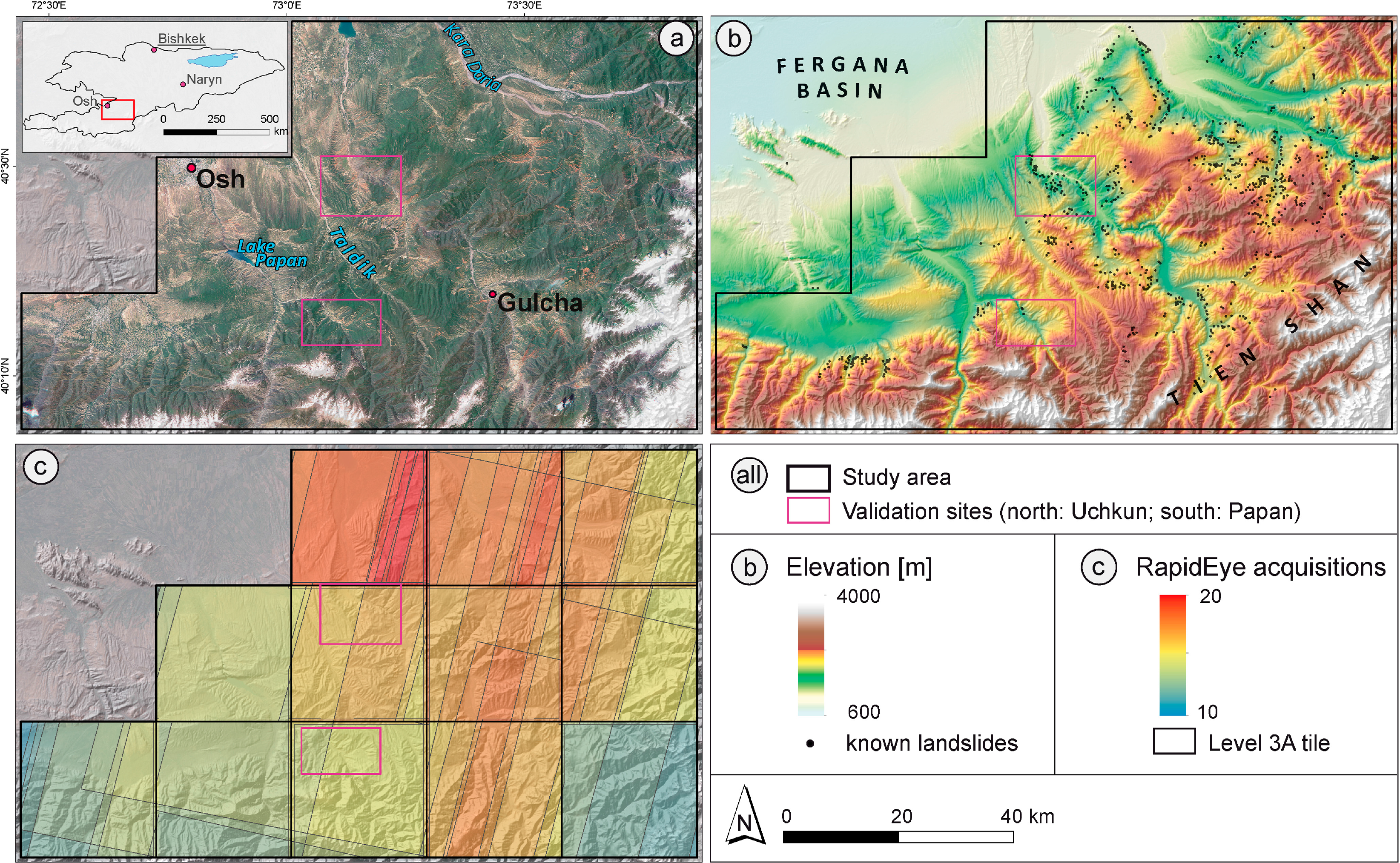
Against this background, the methodological goal of this study is the development of an automated approach for object-oriented landslide mapping of large areas which is suitable for generating multi-temporal landslide inventories, including the possibility for regular monitoring of spatiotemporal landslide activity. For this purpose, a multi-temporal RapidEye [38] remote sensing database of 5 m spatial resolution has been established for a 7500 km2 landslide-affected area in southern Kyrgyzstan for the time period between 2009 and 2013 with up to six multi-temporal acquisitions per year between April and July (Figure 1c). The database contains standard orthorectified Level-3A data products to enable operational applicability of the approach requiring efficient analysis of large amounts of data independent from the availability of ground truth information. The landslide situation in the study area and the spatial database are described in more detail in Section 2, also showing the multi-temporal appearance of different landslide types occurring in the study area. Section 3 describes the developed approach for object-oriented multi-temporal landslide mapping based on temporal NDVI-trajectories covering the whole available time series. Section 4 presents the results obtained by applying this approach to the whole study area. Subsequent systematic accuracy assessment is performed for two independent validation sites that differ in landslide activity and natural conditions (Section 5). In Section 6, the developed approach is discussed in regards to its methodological specifics, achievable accuracy and principle applicability. These are followed by the concluding remarks of Section 7.
2. Study Area and Database
2.1. Study Area and Landslide Situation
In southern Kyrgyzstan, landslides are especially concentrated in the foothills of the high mountain ranges along the eastern rim of the Fergana Basin in an elevation range between 700 and 2000 m (Figure 1b). Most of these landslides occur in form of rotational and translational slides in weakly consolidated Quaternary and Tertiary sediments [13]. They represent complex failures and vary greatly in their size, ranging between several hundred and several million square meters, whereas large events of more than one million cubic meters of displaced material have been frequently occurring. Since the beginning of landslide investigations in the 1950s, about 3000 landslides have been reported by local authorities [39,40]. However, these investigations have been mostly limited to areas in the vicinity of populated places and focused on major events with high destructive potential [41]. Thus, the existing spatiotemporal knowledge on landslide events is incomplete and leaves the need for a systematic multi-temporal landslide inventory as a main prerequisite for objective hazard assessment.
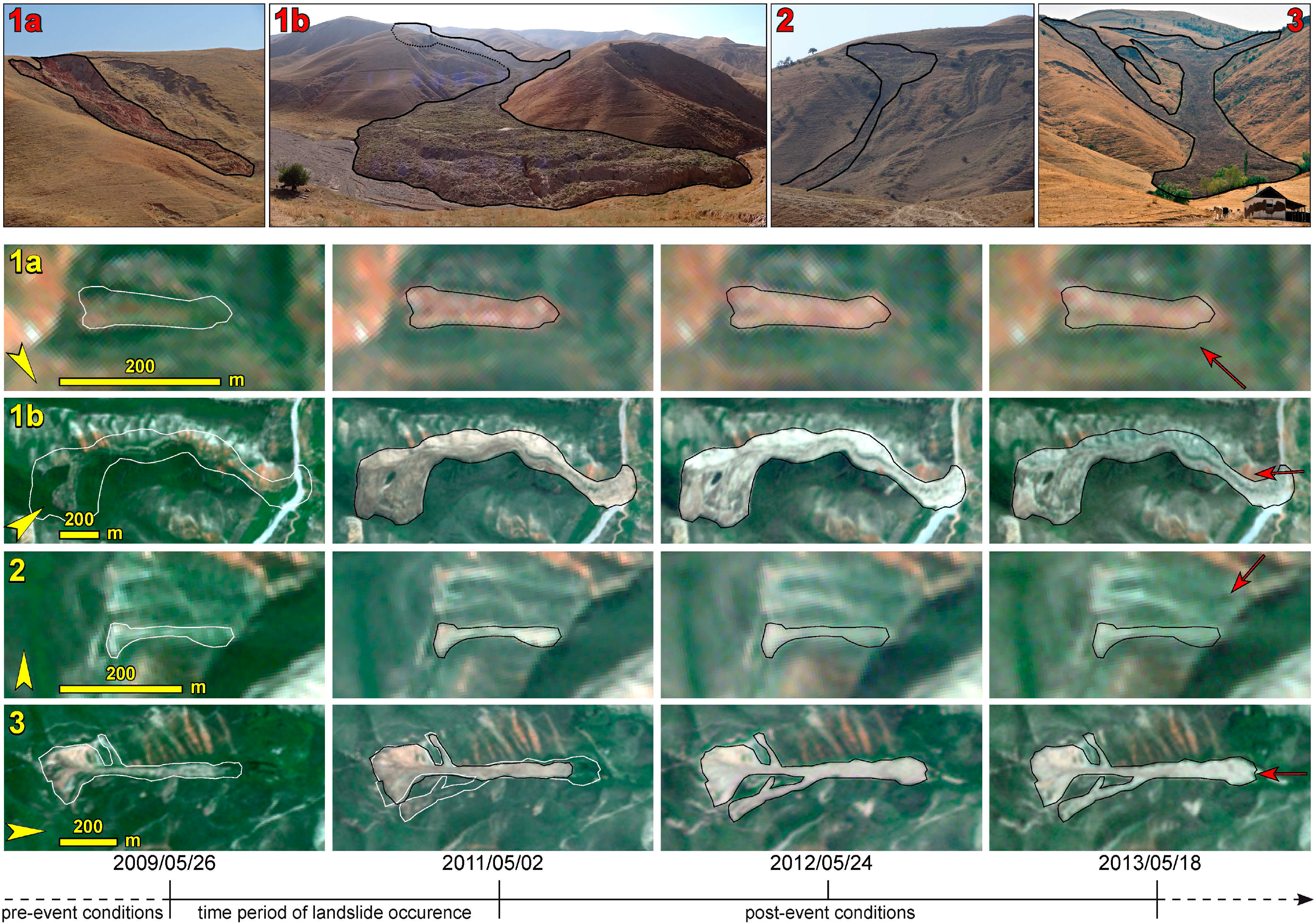
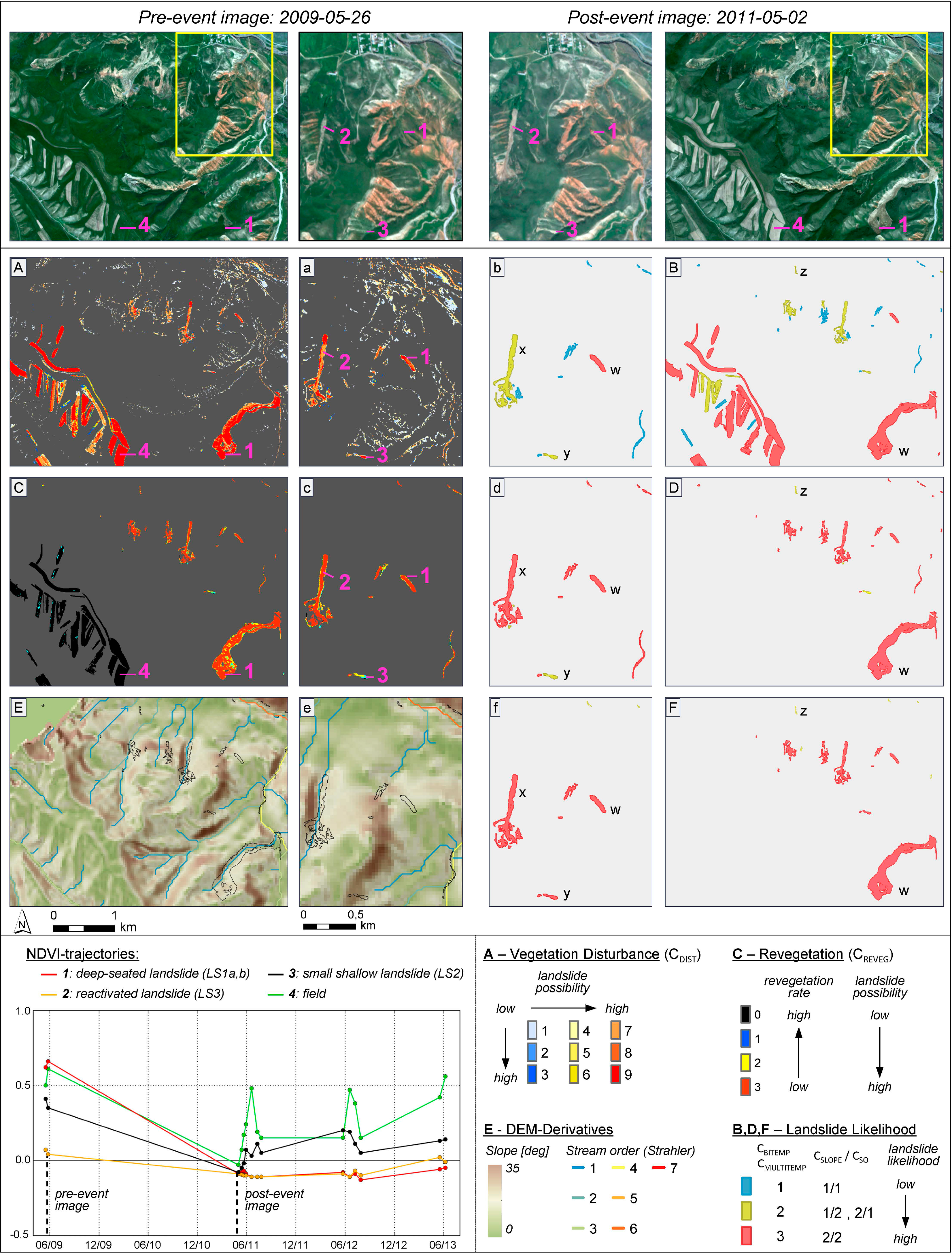
The 7500 km2 study area covered by 12 RapidEye tiles (Figure 1c) is strongly affected by landslides. This region experiences above-average precipitation due to its orographic position west of the topographically rising eastern rim of the Fergana Basin, thus forming a barrier against the prevailing westerlies. The resulting increased precipitation level represents the main factor for the mobilization of landslides in this region. However, this process takes place over longer periods of time and is not related to single triggering events, such as short-term intense rainstorms. The relatively high availability of water leads to a largely developed vegetation cover dominated by grasslands. Therefore, landslide failures cause significant vegetation removal resulting in a distinct contrast between landslides and their surroundings that is easily detectable in optical imagery. Figure 2 illustrates this situation in an exemplary way based on four landslides typical of the whole study area using four multi-temporal RapidEye images contained in the database. All of these landslides occurred in spring 2010 between the depicted RapidEye acquisitions of 26 May 2009 and 2 May 2011. All of them have caused major disturbance of the Earth’s surface and large displacement of material consisting of top soil, as well as underlying weakly consolidated sediments. The resulting destruction of the original vegetated surface cover is clearly visible and largely preserved during the whole depicted post-failure time period.
Field work carried out in the entire study area has revealed that the degree of vegetation destruction and the rate of post-failure revegetation are variable and depend on a number of factors, such as initial vegetation cover, degree of soil disturbance, hydrometeorological conditions, lithology, and state of activity of the landslide. Fresh failures (LS1a,b and LS2) are characterized by a high degree of vegetation destruction due to an undisturbed dense initial vegetation coverage shown by the pre-event image of 26 May 2009. Conversely, reactivations (LS3) are associated with less vegetation destruction because they are typically characterized by sparse and patchy initial vegetation coverage as a result of a former landslide at this position. For all landslides, the post-failure revegetation is typically very slow, as the landslide masses are susceptible to erosion and reactivation processes. In the case of the depicted deep-seated landslide examples (LS1a,b and LS3), hardly any revegetation can be seen in the image acquired three years after the failure (18 May 2013), whereas the shallow landslide LS2 is characterized by faster revegetation.
2.2. Remote Sensing Database and Pre-Processing
The multi-temporal optical remote sensing database consists of 216 orthorectified Level-3A RapidEye datasets delivered in the form of 25 × 25 km2 tiles with 5 m pixel size. They have been provided by the RapidEye Science Archive (RESA) data grant program which has allowed customized data acquisition in pre-defined time periods of high landslide activity. As a result, a high temporal resolution of up to six acquisitions during the growing season between April and July could be achieved. Together with archive data acquired in 2009, there was a result of up to 20 acquisition dates between the years of 2009 and 2013, whereas no acquisitions were performed in 2010 (Figure 1c). The resulting high temporal resolution allows the determination of the time period of landslide occurrence up to several days and weeks, which is important for spatiotemporal analysis of landslide activity in respect to triggering and predisposing factors. Besides the multispectral remote sensing data, the developed landslide mapping approach is also based on a digital elevation model (DEM) of 30 m spatial resolution derived from the X-band data of the Shuttle Radar Topography Mission in February 2000 [42]. The DEM is used to derive landslide-related geomorphological information for the study area as contextual information for more reliable object-oriented landslide mapping (Section 3.2.3).
2.3. Pre-Processing of Remote Sensing Data
Pre-processing aims at the reduction of artifact changes in subsequent time series analysis. Such artifact changes are introduced by geometric mismatches and radiometric differences between the image data sets, as well as pseudo-surface cover changes introduced by the temporary presence of clouds and snow [43,44]. To foster the potential for operational use and taking into account the high number of datasets, pre-processing has to be performed in an automated, robust and efficient way. For geometric adjustment, an image-to-image co-registration approach has been developed that allows automated spatial alignment of time series data comprising orthorectified standard data products [45]. As a result, geometric offsets of up to 60 m between the multi-temporal image data have been corrected and a relative image-to-image co-registration accuracy of less than one 5 m RapidEye pixel could be achieved for the complete multi-temporal database. To reduce the effects of radiometric differences between the images for subsequent change detection analysis, the developed landslide mapping approach (Section 3) is based on the temporal comparison of the normalized difference vegetation index (NDVI) derived from the standard corrected top-of-atmosphere radiance data. The remaining variability in NDVI values between the multi-temporal datasets needs to be compensated by the developed approach (Section 3.2). For masking clouds and snow, a threshold has been applied to the blue band of the RapidEye images (Band1BLUE > 1050 W·m−2·sr−1·µm−1). This threshold based approach has been extended by analyzing the whole time series in order to separate between permanent bright objects (e.g., sand and urban objects) and temporary ones (clouds and snow). In this context, it is assumed that a permanent bright object is present in all images of the time series, whereas clouds and snow are only temporarily present. This way even less thick cloud cover could be identified.
2.4. Reference Mapping for Validation Sites
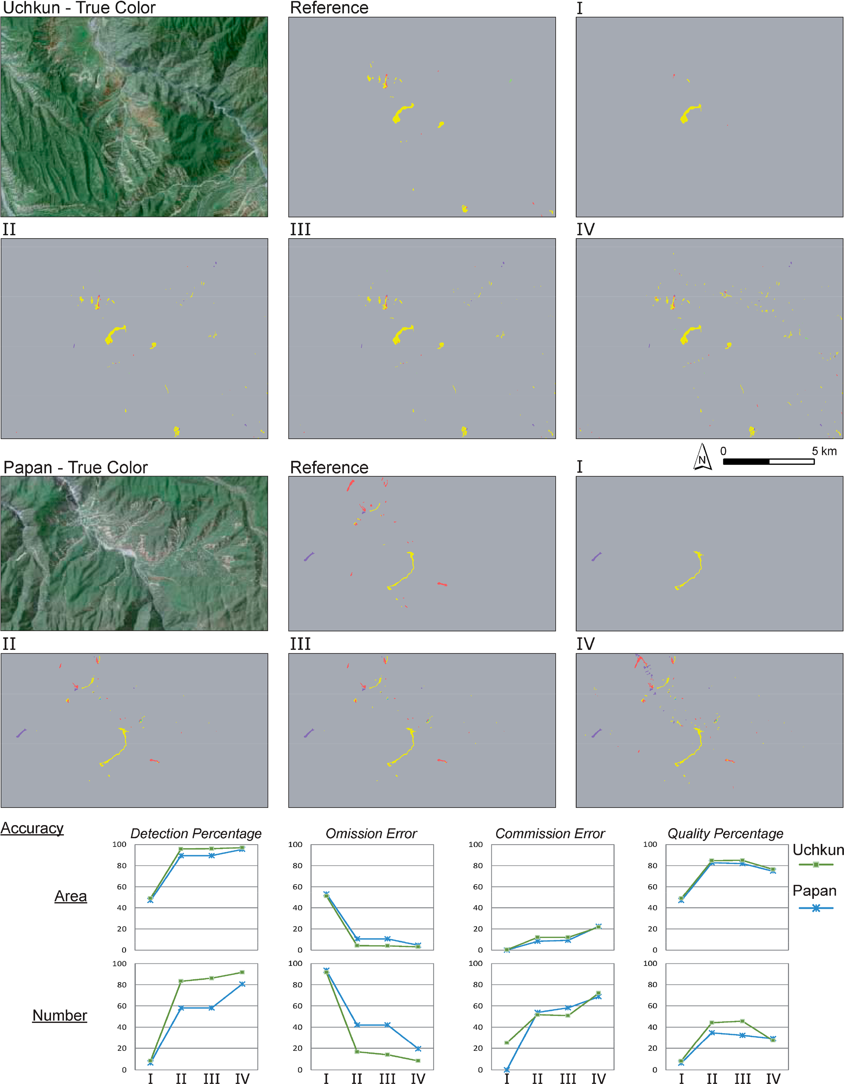
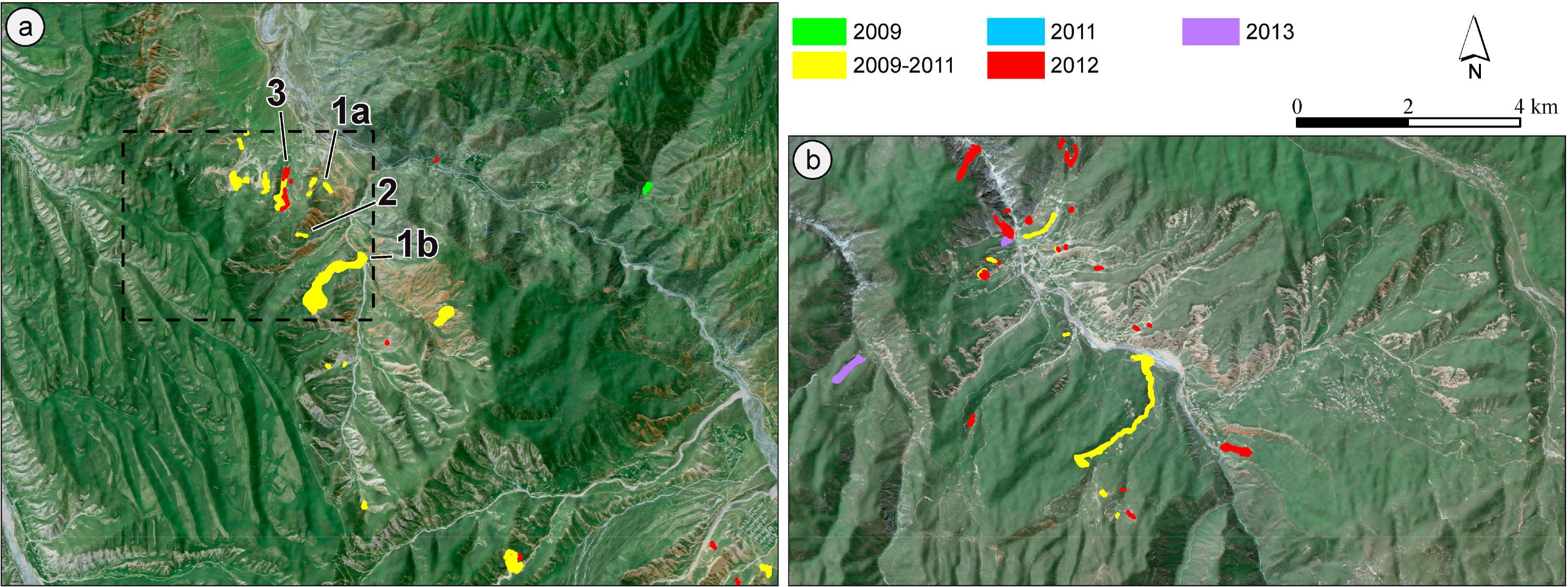
To quantitatively assess the accuracy of object-oriented landslide mapping resulting from the developed approach, reference mapping has been carried out for two spatially independent validation sites which have been affected by recent multi-temporal landslide activity. They are outlined in Figure 1 and represent contrasting environments which are representative for the whole study area. The size of these validation sites amounts to approximately 14 × 11 km2 for the site Uchkun (Figure 3a) and 14 × 8 km2 for the site Papan (Figure 3b). The land use in these two sites is dominated by pastures and grassland. However, they also comprise several non-vegetated areas which could be mistaken for landslides, because of their similar appearance in optical remote sensing data. Both validation sites contain small settlements along the valleys close to the river beds. The Uchkun site further covers a bigger village in the southeastern part and an area of crop cultivation (western part), temporally without vegetation cover due to harvesting. The Papan site comprises a high percentage of permanently non-vegetated steep outcrops appearing as bright areas mainly in the center of the validation site. Furthermore, the two sites also differ in available remote sensing data, due to their location in different Level-3A RapidEye tiles (Figure 1c).
For both validation sites, a reference landslide inventory has been created by visual interpretation of the available RapidEye data acquired between 2009 and 2013, whereas the time period of occurrence of a mapped landslide is determined by the time period between the pre- and post-event RapidEye image. In Figure 3, these time periods are classified into full years, whereas the acquisition date of the post-event image defines the depicted year of occurrence. An exception is caused by the missing RapidEye acquisitions in 2010 resulting in a class of landslide occurrence between 2009 and 2011. Manual reference mapping has also been supported by spatially very high resolution satellite remote sensing data contained in the Google Earth™ archive with most recent images acquired in June 2013 for both validation sites. Furthermore, these inventories were validated during a field survey in September 2012. In total, 67 landslides were mapped—36 in the Uchkun and 31 in the Papan site. The size of these landslides ranges between 500 and 250,000 m2, whereas the total area affected by landslides amounts to approx. 1 km2. Both sites are characterized by spatial and temporal concentrations in landslide occurrence, as well as areas and time periods without landslide activity. The Uchkun site is most strongly affected between the years 2009 and 2011, whereas for the Papan site highest landslide activity could be observed for 2012. Thus, the two selected validation sites differ in spatiotemporal landslide occurrence as well as in natural conditions and available RapidEye data coverage, thereby making them suitable for representative accuracy assessment of the developed approach.
3. Automated Approach for Multi-Temporal Landslide Mapping
The methodological developments aim at the automated multi-temporal mapping of landslides based on satellite remote sensing time series data. Thus, the approach needs to be able to identify landslide activations occurring at different times during the analyzed time span, whereas the determination of the time of landslide occurrence depends on the length of the time period between two subsequent images contained in the remote sensing time series database. To meet the goal of generating a multi-temporal landslide inventory, the approach is required to derive the occurring landslides as single objects for each of these time periods. In this context, the approach needs to take into account the natural variability of landslide phenomena occurring within the large study area.
To fulfill these requirements, the developed approach builds on a pixel- and object-oriented analysis of temporal NDVI-trajectories enabling the incorporation of rule-based knowledge about landslide-related surface cover changes. Furthermore, the approach comprises the possibility for the discrimination between uncertainty-related landslide likelihood classes to enable expert-aided evaluation of the results suitable for different applied tasks related to landslide investigations. For clarity, the descriptions of the basic idea (Section 3.1) and of the knowledge-based system (Section 3.2) are based on the exemplary analysis of the two subsequent RapidEye acquisitions (26 May 2009 and 2 May 2011) within the 8 × 4.5 km2 subset depicted as dashed line in Figure 3a. In Section 3.3, the developed approach is extended to the whole time series available for this exemplary subset to demonstrate the derivation of the final results of multi-temporal landslide mapping. All methodological developments are realized using the open source programming language python.
3.1. Temporal NDVI-Trajectories for Landslide Identification
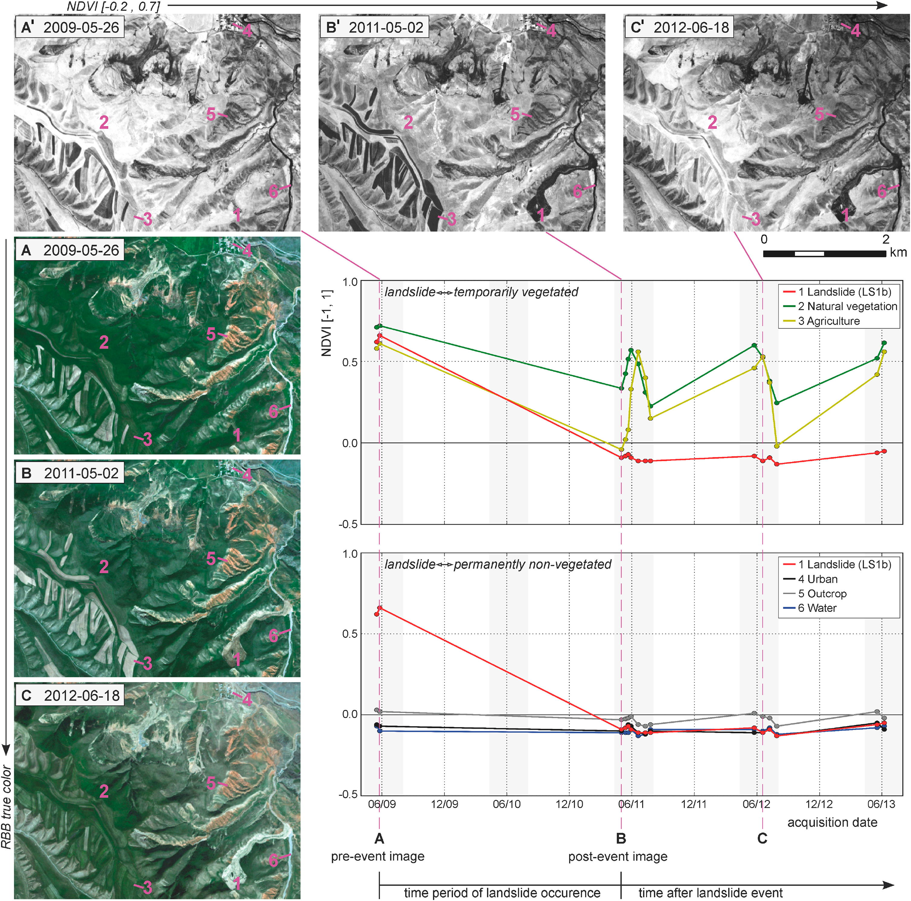
Temporal NDVI-trajectories represent specific temporal footprints of vegetation changes which are obtained for every pixel across the time span of the analyzed multi-temporal data stack. Figure 4 illustrates how these NDVI-trajectories can be used to distinguish between landslide-related vegetation changes (Figure 4(1)) and five other land cover changes (Figure 4(2–6)). In the case of the depicted landslide example LS1b, which occurred in the spring of 2010 (Figure 2(LS1b)), the failure caused a severe vegetation cover disturbance that is reflected in the abrupt decrease of the NDVI values between the RapidEye acquisitions of 26 May 2009 and 2 May 2011. These low post-failure NDVI values have been maintained for the following two years, indicating a slow revegetation rate in the area of the displaced landslide masses (Section 2.1). Based on the resulting distinct temporal NDVI-trajectory, landslides can be distinguished from permanently non-vegetated areas (Figure 4, bottom) characterized by permanent low NDVI values, as well as from temporally vegetated areas (Figure 4, top) characterized by a less distinct NDVI decrease and/or faster revegetation rates.
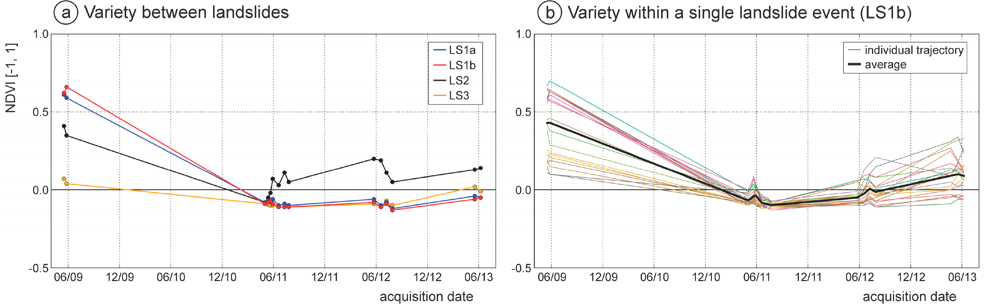
Compared to the ideal case of the fresh failure LS1b, other landslides may result in less distinct vegetation changes. Figure 5a illustrates such less-pronounced differences by depicting one characteristic NDVI-trajectory for each of the four landslide examples shown in Figure 2. If mass movements represent reactivations, which are typically occurring in areas of already existing landslides (Figure 2(LS3)), a smaller decrease of the NDVI values can be observed because of the sparser vegetation cover before failure. In the case of small shallow landslides (Figure 2(LS2)), the revegetation rate is often faster, because of the less severe soil disturbance. In the case of the deep-seated landslides (LS1a and LS1b), the NDVI-trajectories are very similar, showing their independence from the lithological properties of the material involved in the landslide failures. Besides the differences between the respective landslides, the temporal vegetation change characteristics also differ within a single landslide. Figure 5b depicts NDVI-trajectories for 20 pixels within landslide LS1b showing differences in the bi-temporal NDVI decrease and rate of post-failure revegetation. However, despite all of the described differences, the typical shape of a landslide-specific NDVI-trajectory is still maintained.
3.2. Processing System for Knowledge-Based Landslide Identification
Based on the temporal NDVI-trajectories, a combined pixel- and object-oriented approach has been developed for the automated identification of landslide occurrence for subsequent image pairs, taking into account the entire available time series. For this purpose, the approach analyzes the degree of bi-temporal vegetation changes serving as the basis for the segmentation of landslide candidate objects for each time period (Section 3.2.1). In the following, these landslide candidate objects are evaluated regarding their plausibility in terms of post-event multi-temporal revegetation (Section 3.2.2) and relief-oriented parameters (Section 3.2.3). Figure 6 exemplarily illustrates the derivation of parameters that are used in the temporal NDVI-trajectory analysis. Figure 7 shows the overall processing scheme of the developed approach subdividing these three major parts into the processing steps A–F. The description in Section 3.2 follows steps A–F, whereas the empirically determined thresholds for each step are listed at the right of Figure 7. Figure 8 illustrates the results of each processing step based on the subset area shown in Figure 4. In the final step of the approach (Section 3.2.4), the object-oriented results are evaluated by the introduction of a reliability classification in the form of the overall landslide likelihood.
3.2.1. Derivation of Landslide Candidate Objects Based on Bi-Temporal Vegetation Change Analysis
A: Pixel-Oriented Bi-Temporal Change Detection
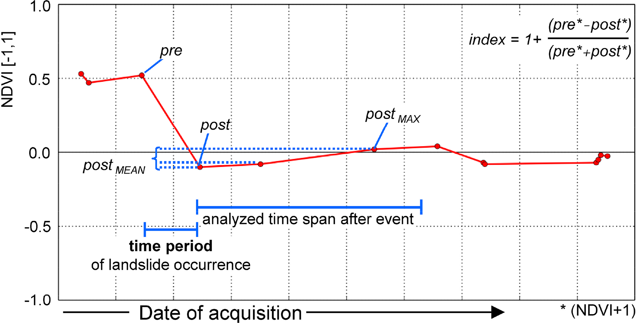
To classify the bi-temporal vegetation disturbance for each pixel (CDIST) in regards to the possibility of landslide occurrence, the NDVI values after an expected landslide (post) and the normalized index of the NDVI values of the pre-event and post-event image (index) are used in combination (Figures 6 and 7). As shown in Figure 4, landslides usually cause the total loss of previously existing vegetation, which results in high index values and post values of less than zero representing bare soil. However, to accommodate the variety of landslide processes (Figure 5), the bi-temporal analysis of vegetation disturbance (CDIST) is performed on a scale of 9 classes (Figure 7). The main idea of this multiple threshold-based analysis is adapted from the robust differencing approach developed by Castilla et al. [46]. The usage of multiple thresholds also enables the identification of less-pronounced surface cover changes related to landslide occurrence, e.g., if the vegetation cover is already less dense before the landslide event (e.g., Figure 2(LS3)). Figure 8A illustrates the results of this classification. The pixels representing deep-seated landslides (Figure 8(1)) have been classified with the highest CDIST class of 9 and the landslide pixels characterized by less distinct bi-temporal vegetation changes (Figure 8(2,3)) have been assigned to lower CDIST classes. However, the classification has also led to a high percentage of false-positive pixels that are introduced by slight vegetation changes in sparsely vegetated areas mainly in the northeastern part and by a distinct vegetation loss in the area of harvested fields in the western part of the subset shown in Figure 8. The exemplary NDVI-trajectory for harvested fields (Figure 8(4)) shows bi-temporal changes that are very similar to the ones of the deep-seated landslides (Figure 8(1)) and thus results in the same CDIST classes.
B: Object-Oriented Classification of Bi-Temporal Landslide Likelihood
Based on the pixel-oriented results of the first step, a subsequent segmentation is performed that extracts individual segments from all of the spatially 8-connected pixels which have been assigned to a vegetation disturbance class (CDIST > 0). The segments are classified regarding their bi-temporal landslide likelihood (CBITEMP) by analyzing the frequency of the CDIST classes for all pixels contained in the segment. If the segments do not meet any of the landslide likelihood criteria shown in Figure 7 (CBITEMP = 0), they represent segments containing an excessively high percentage of pixels characterized by vegetation changes not typical for landslide occurrence; they are therefore eliminated. All other segments are kept as landslide candidate objects characterized by a three-step bi-temporal landslide likelihood (CBITEMP = 1–3) of ascending order (Figure 8B). This procedure ensures the derivation of landslides as single objects even if in part they do not represent the optimal case of a significant vegetation disturbance. At the same time, this procedure reduces the high number of pixels with slight vegetation changes that can be considered as noise. Figure 8B shows that the deep-seated landslides (Figure 8(1,w)) are classified with the highest bi-temporal landslide likelihood (CBITEMP = 3) because their segments consist of more than 30% of pixels with the highest bi-temporal vegetation disturbance class (CDIST = 9). The reactivated landslide (Figure 8(2,x)) and the shallow landslide (Figure 8(3,y)) are classified with lower bi-temporal likelihood values (CBITEMP = 2). Furthermore, Figure 8B shows the reduction of false-positive pixels, especially in the northeastern part of the subset.
3.2.2. Multi-Temporal Revegetation Analysis
C: Pixel-Oriented Multi-Temporal Change Detection
For each pixel contained in the identified objects, the revegetation is analyzed within a user-defined time span allowing the differentiation between landslide-related slow revegetation and other vegetation cover changes. In this study, this time span is limited to a maximum of three years, because the vegetation usually starts to recover in most parts of the landslides after these three years. Based on all post-event images available in this time span, the degree of revegetation is classified into four rates of revegetation (CREVEG). They are based on the maximum (postMAX) and mean NDVI values (postMEAN) derived from the NDVI-trajectory (Figure 6). The combination of postMAX and postMEAN allows a robust determination of the revegetation rate (Figure 7). In contrast, the single use of postMAX would be susceptible to co-registration errors, which could result in high NDVI values at the edge of landslide objects if the landslide is surrounded by vegetation. The single use of postMEAN would be more susceptible to the date of the image acquisitions and could result in rather low NDVI values for fields if the field is harvested in the majority of the acquired datasets. Figure 8C shows a reliable differentiation between landslide-related surface changes and fields resulting from the revegetation rate classification. The pixels of the fields are characterized by revegetation rates higher (CREVEG = 0) than the landslide pixels (CREVEG = 2 or 3).
D: Object-Oriented Classification of Multi-Temporal Landslide Likelihood
Based on the frequency of the pixel-oriented revegetation rate classes (CREVEG), the landslide candidate objects are further characterized in regards to their multi-temporal landslide likelihood (CMULTITEMP). Following the procedure described in (B), all landslide candidates are eliminated that do not meet any of the criteria shown in Figure 7 (CMULTITEMP = 0) and the remaining objects are classified into three likelihood classes (CMULTITEMP = 1–3). Thus, fields are eliminated from the landslide candidates, whereas landslides are maintained (Figure 8D). This way, landslides of low revegetation rates (Figure 8((1,w),(2,x))) and also landslides of faster natural revegetation (Figure 8(3,y)) could be distinguished from fields, whereas the shallow landslide (Figure 8(3,y)) is characterized by slightly lower multi-temporal landslide likelihood (CMULTITEMP = 2).
3.2.3. Relief-Oriented Analysis
E, F: Pixel- and Object-Oriented Analysis of Relief Parameters
Landslide candidate objects are further evaluated in regards to relief-based plausibility based on the two parameters: slope and parallelism to streams (Figure 7). The first parameter slope has already been widely used for this purpose [20,21,24,28,29,35]. It takes into account the fact that landslides require a certain initial relief contrast to allow the downward movement of material as a result of the onset of a slope failure. In this study, landslide objects are required to be characterized by an average slope (slopeMEAN), ranging between 7° and 30°. However, this range is only applicable to the source area of a landslide, since the accumulation zone can also comprise flatter parts resulting in slope values below the thresholds implemented for slopeMEAN. Therefore, the approach also analyzes the proportions of the slope values (slopeHIST) within the landslide object. If at least 50% of the slope values are larger than 8°, the object is still considered a landslide. Both parameters (slopeMEAN, slopeHIST) are combined to a slope-oriented parameter (CSLOPE) for the evaluation of each landslide candidate object.
The second parameter, parallelism to streams, aims at eliminating false positives which occur if a river has flooded a formerly vegetated area or if local co-registration errors between the pre- and post-event images result in changes which have the same appearance as the ones in the flooded areas. An example is shown in the lower right part of Figure 8e. Analysis of a landslide object being parallel to streams is based on the distance and orientation of that object in regards to the stream network (Figure 7) derived from a DEM using the stream order by Strahler [47]. The orientation of the landslide object and the corresponding part of the adjacent stream is calculated by using the major axis of the ellipse, which is defined by the second central moment of the analyzed region [48]. First-order streams are excluded from this analysis because landslides are often occurring alongside these topographically less pronounced valleys. For all other streams belonging to higher orders, the objects are evaluated in three steps (Figure 7) according to the degree of parallelism (CSO), whereas CSO = 2 represents the highest degree of being parallel. Both object parameters (CSLOPE, CSO) are combined into the relief-oriented landslide likelihood (CRELIEF). If the landslide candidates are either clearly parallel to a stream (CSO = 2) or do not meet any of the slope criteria (CSLOPE = 0), they are classified as false positives. Applying this procedure, the object in the southeastern part of the enlarged zoom area of Figure 8e, which is parallel to a fourth-order stream, is eliminated from the identified landslide candidates shown in Figure 8f. The remaining landslide candidates are characterized by the three-step relief-oriented landslide likelihood parameter (CRELIEF) illustrated in Figure 8F.
3.2.4. Classification of Overall Landslide Likelihood
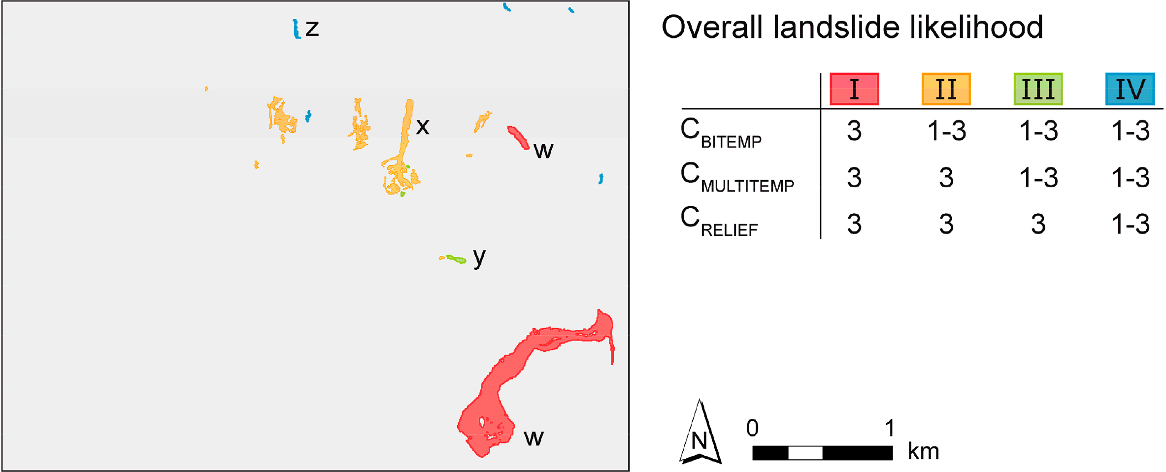
To obtain meaningful results in the process of automated landslide identification—comprising the existing variability of landslide phenomena and the possibility for subsequent evaluation of the results by landslide experts—the identified landslide objects are classified into four (I–IV) classes representing different degrees of overall landslide likelihood (Figure 9). These classes are an expression of the level of uncertainty related to the automated identification of this particular landslide object using the three previously described parameters CBITEMP, CMULTITEMP and CRELIEF. Class I represents the ideal case of a deep-seated fresh failure which is characterized by high bi-temporal vegetation loss (CBITEMP = 3), very low revegetation rates (CMULTITEMP = 3) and very high relief oriented landslide likelihood (CRELIEF = 3). Both deep-seated fresh landslides LS1a and LS1b (object w in Figures 8 and 9) are characterized by the highest overall landslide likelihood. The reactivated landslide LS3 (object: x) is characterized by less distinct vegetation loss (CBITEMP = 2), but it still performs to an ideal in terms of the other two parameters and is thus classified into the overall landslide likelihood class II. Additionally to the non-ideal bi-temporal vegetation changes of class II, class III comprises also non-ideal revegetation rates. The small shallow landslide LS2 (object: y) represents an example for this case, which is characterized by likelihood parameter values of 2 for both CBITEMP and CMULTITEMP. In the case of the lowest landslide likelihood class IV, objects are characterized by non-ideal values (<3) for all three parameters. The object z in Figures 8 and 9 represents an example for such cases. Overall, this demonstrates that these landslide likelihood classes represent the level of uncertainty as well as, to a certain degree, the type of landslide activation.
Furthermore, these overall landslide likelihood classes enable the separation of the automatically derived landslide mapping results into four selection categories (I–IV) representing a selection of the results of varying levels of strictness. In this context, the selection category IV represents the least strict selection and comprises all automatically mapped objects independent from the assigned overall landslide likelihood class. In contrast, category I solely comprises the objects belonging to the highest landslide likelihood class representing the most strict selection. In Section 5, the results of these selection categories are evaluated in regards to mapping accuracy, thereby showing how these categories influence the approach in terms of automated or semi-automated usage.
3.3. Multi-Temporal Landslide Mapping for Whole Time Series
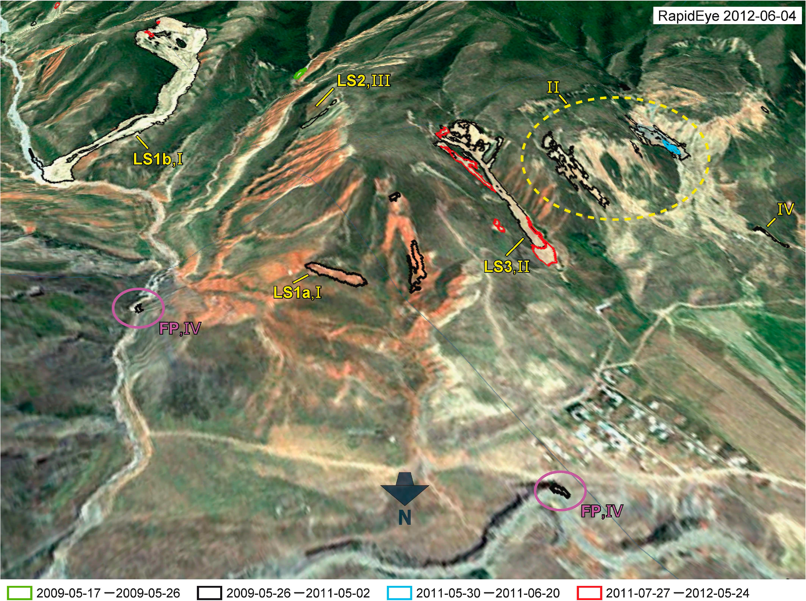
The application of the approach to the whole RapidEye time series has resulted in the identification of landslide events in four out of the 15 subsequent image pairs (Figure 10). The length of the identifiable time period of landslide occurrence depends on the temporal resolution of the available RapidEye time series data. In the case of the methodological subset, it varies between nine days (17 May 2009–26 May 2009) and two years (26 May 2009–2 May 2011). The results reveal the suitability of the approach for the identification of landslides representing fresh failures and reactivations (Section 2.1). In Figure 10, fresh failures are represented by the landslides LS1a, LS1b, and by the green polygon. Reactivations are shown by the polygons within the yellow ellipse and the landslide LS3. In the case of landslide LS3, two reactivations could be identified that both resulted in an enlargement of the crown area of the landslide and caused a further downward displacement of the already accumulated material. Moreover, Figure 10 also shows that the automated identification is independent from the lithology of the affected slopes, whereas the majority of the identified landslides occurred within loess (bright areas) and some within weakly consolidated reddish sedimentary rocks (e.g., LS1a).
The exemplary results show that the approach is capable of reliable identification of landslides occurring during the analyzed time span (2009–2013) and distinguish them from older landslides that were already present. Furthermore, Figure 10 also confirms the suitability of analyzing temporal NDVI-trajectories for the separation between landslide objects and other non-vegetated areas, such as buildings, streets, outcrops and river beds. However, the purple ellipses shown in Figure 10 indicate two falsely identified landslide objects representing false positives (FP) in the specific form of small erosion features at a riverbank. To evaluate the influence of such identification errors on the overall quality of the automated landslide mapping result, a quantitative accuracy assessment was performed and is outlined in Section 5.
4. Application of Approach to Whole Study Area
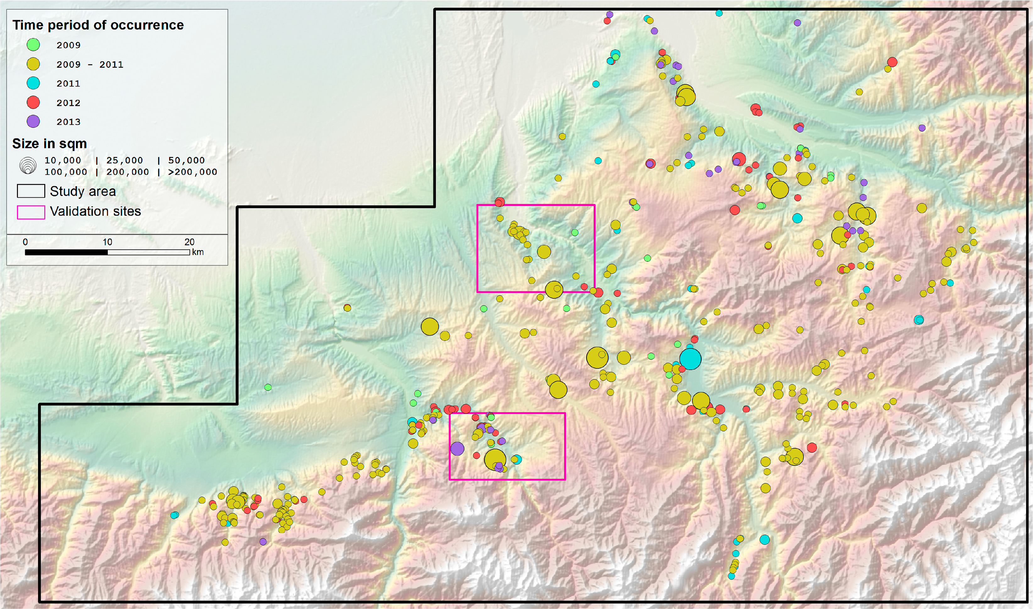
Automated multi-temporal landslide mapping has been performed for the whole study area, which is characterized by variations in natural conditions and temporal RapidEye data coverage (Section 2). The complete mapping result, which includes objects of all overall landslide likelihood classes, has been visually validated by landslide experts to remove obvious false positives. All automatically identified landslides could therefore be included in the overall evaluation of the spatiotemporal landslide activity. As a result, 471 landslides have been identified, whose location, classified size, and time period of occurrence is depicted in Figure 11. During field investigations in September 2012, 120 of these identified landslides were visited, only revealing four false identifications. Each of these cases represented a manmade removal of construction material in the lower part of a slope.
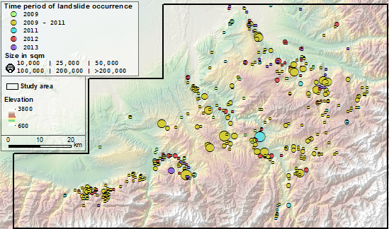
The size of the identified landslides ranges between 125 and 750,000 m2, and the total area affected by these landslides amounts to 6.1 km2 (Table 1). Table 1 also shows the distribution of the temporal landslide activity in respect to the classified time periods. The longest analyzed time period between 2009 and 2011 comprises 55% of all identified landslide objects. Landslide activity is less intense in the other analyzed years, varying between 6% of occurred landslide events in 2009 and 18% in 2012. These findings reveal a constantly ongoing landslide activity independent from major triggering events, such as intense rainstorms or larger earthquakes that did not happen in this region during the analyzed time period between 2009 and 2013. Moreover, the spatial distribution of the landslide objects depicted in Figure 11 shows clear spatial variations in landslide activity, including areas of distinct concentrations, whereas most landslides occurred at elevations between 900 and 2300 m. For this region, the obtained results comprise the first systematic assessment of spatiotemporal landslide activity, thus representing a main prerequisite for objective hazard and risk assessment.
5. Accuracy Assessment
The systematic accuracy assessment of the developed approach is performed for two independent validation sites (Section 2.4). Section 5.1 assesses the influence of the landslide likelihood-based selection categories on the quantitative accuracy of the landslide mapping results. In Section 5.2, the accuracy assessment is complemented by the evaluation of the geometric quality of the automatically identified landslide objects.
5.1. Quantitative Landslide Mapping Accuracy
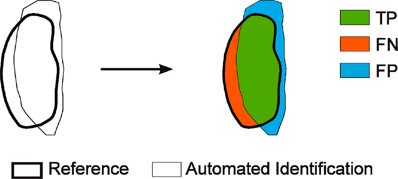
To obtain a comprehensive quantitative evaluation of the approach, the conformity between automated identification and reference mapping is analyzed for both validation sites and for each selection category (I–IV) in regards to the number of landslides and the area affected by these landslides. This comparison results in one of three relevant identification categories: true positive (TP), false negative (FN), and false positive (FP). TPs comprise the correctly mapped landslides, whereas the other two identification categories represent two types of identification errors. FNs correspond to reference landslides that have not been identified by the approach, and FPs are identified landslide objects which have not been mapped in the reference inventory. The fourth identification category of true negatives (TN) does not apply in the case of object-based single-target classifications [29].
To evaluate the performance of the landslide mapping approach the three relevant identification categories have to be considered in relation to each other. The best result is characterized by 100% TP and absent identification errors (0% FP and 0% FN). Based on this relation, the four accuracy metrics, Detection Percentage, Omission Error, Commission Error and Quality Percentage [29,49,50], are selected for the comprehensive accuracy assessment:
The Detection Percentage—also called True Positive Rate or Producer Accuracy—represents the percentage of landslides which have been correctly identified by the automated approach. The Commission Error and the Omission Error describe separately the influence of the two possible identification errors FP and FN, respectively. The Quality Percentage represents an integrative indicator and relates the correctly mapped landslides to both possible identification errors, indicating how likely a landslide is correctly identified.
Figure 12 illustrates in a spatially explicit way the results of the four different selection categories for both validation sites in comparison to the reference mapping. At the bottom of Figure 12, the performance of each selection category is shown in terms of the four accuracy metrics (Equations (1)–(4)), which are calculated based on the accuracy statistics shown in Table 2. The less strict selection categories result in higher Detection Percentages with a maximum of up to 95% correct identification of the landslide-affected area and more than 80% of the number of landslides achieved by selection category IV. Thus, category IV is most suitable to minimize missing identifications (FN) and to obtain results that comprise most of the landslide occurrences, including landslides that are characterized by very slight vegetation cover changes, represented by reactivations of already existing landslides or very small and shallow landslides. However, applying less strict selection categories, the number of FPs increases, which is expressed by the higher Commission Errors. Therefore, the mapping results of category IV are most suitable for subsequent evaluation by a landslide expert who can interactively eliminate the FPs. This way, the least strict selection category minimizes the likelihood that potentially dangerous landslide objects are not included in the automated mapping result. In contrast, category I results in the complete absence of FP for the Papan site and only a single FP object of 900 m2 size for the Uchkun site. Thus, category I minimizes the number of FPs and limits the automated identification results to correctly identified landslide objects (TP) that are most likely to represent fresh landslide failures. Hence, if only landslide objects that represent most recently occurred new landslides are of interest, the selection category I can be used.
However, to apply the approach to large areas in a fully automated way, the approach needs to counterbalance the influence of the two identification errors (FP, FN). The integrative Quality Percentage takes this into account and shows the highest values for categories II and III in both validation sites. As a result, the application of these categories results in correct landslide identification for more than 90% of the landslide area, accompanied by Omission and Commission Errors of around 10%.
Furthermore, the findings of the accuracy assessment show that the quality of the results is higher regarding the landslide-affected area than compared to the number of landslides. In the case of selection category II, the Quality Percentage amounts to approx. 80% for the area and approx. 40% for the number of landslides. This difference reveals that the approach identifies larger landslides with higher reliability and that both identification errors (FN, FP) are mostly caused by objects of smaller spatial extents.
5.2. Evaluation of the Geometric Quality of the Landslide Object Delineation
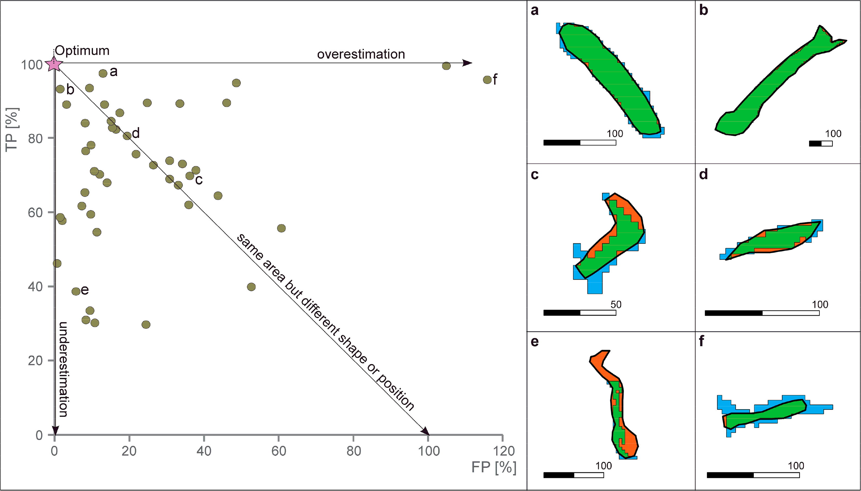
The correct spatial delineation of the automatically identified objects is important for the generation of high-quality multi-temporal landslide inventories which are required for subsequent objective hazard analysis. For this purpose, all of the 58 landslide objects which were correctly identified for the two validation sites have been individually compared to the reference mapping objects in regards to the degree of their spatial overlap (Figures 13 and 14). As a result, spatially explicit representations of the true positive (TP), false negative (FN) and false positive (FP) areas have been obtained for each object comparison (Figure 14). Their normalization by the size of the respective reference objects (sum of TP and FN) results in percentages for all of these three parameters. As such, the ideal spatial overlap between two objects is represented by 100% TP and 0% FP indicated by the star in the diagram of Figure 14 depicting the individual objects regarding their percentages of TP and FP. Based on this optimum situated at the origin of the diagram, three typical object delineation errors could be identified. Along the y-axis, the percentage of the correctly mapped landslide area is further reduced, thereby corresponding to a progressing underestimation of the size of the automatically derived objects compared to the size of the reference objects. Along the x-axis, the percentage of the FP area increases and results in an overestimation compared to the reference mapping. Along the line depicted in the diagram, the automatically mapped object corresponds in size to the reference object but differs either in shape or in position compared to the reference object.
Overall, the results depicted in Figure 14 show that most of the analyzed objects are located in the upper left part of the diagram close to the optimum point. The examples a and b in Figure 14 represent two cases of almost ideal object delineations. Another concentration can be seen along the depicted line of the diagram. It can be explained by the fact that automatically pixel-based object delineation always slightly differs from the manually digitized objects. This is especially evident in the case of small objects paradigmatically shown by the examples c and d of Figure 14. The examples e and f represent outliers of less exact object delineation for underestimation and overestimation, respectively. However, the diagram shows that for the vast majority of the analyzed landslide objects, the spatial overlap corresponds to at least 50% in regards to the original object contained in the reference mapping.
6. Discussion
The developed automated approach for spatiotemporal landslide mapping enables comprehensive assessment of landslide activity over longer periods of time. It is based on the analysis of landslide-specific vegetation changes using temporal NDVI-trajectories derived from optical remote sensing time series data complemented by relief parameters. To perform robustly over large areas, the approach considers the existing variability of vegetation change characteristics related to different types of landslides (Figure 5a) and to different parts within a single landslide (Figure 5b). This allows the identification of fresh and reactivated landslide occurrences including their separation from other surface changes not related to landslide processes (Figure 4). In this context, the approach differentiates the identified landslide objects by their overall landslide likelihood, enabling landslide experts to incorporate the level of uncertainty in the subsequent interpretation and evaluation of the results obtained by the automated analysis.
To meet the goal of assessing the multi-temporal landslide activity, the approach derives objects of landslide activations which occurred at different times during the time span of analysis. For this purpose, the segmentation of landslide candidate objects builds on the result of a specific multi-threshold-based change detection analysis considering distinct and less pronounced landslide-related vegetation cover changes between each subsequent image pair contained in the remote sensing time series database. In contrast, the existing object-oriented landslide mapping approaches use mono-temporal information for the segmentation procedure [20,33–37] and thus are not designed to delineate active parts of a landslide. To evaluate the plausibility of the landslide candidate objects of the developed approach, they are further analyzed in regard to relief parameters and post-event rates of temporal revegetation. Analyzing landslides in regards to their relief position has long been a standard part of remote sensing-based landslide recognition [24,51]. However, the incorporation of revegation rates, derived by the analysis of the temporal NDVI-trajectories, has firstly been applied and allows separation of slower revegetation rates typical for areas affected by landslides from other areas characterized by faster revegetation, as in the case of agricultural fields.
The application of the developed approach to the whole study area (Section 4) has confirmed its suitability for supporting the generation of multi-temporal landslide inventories for large areas. In this context, the approach enables the analysis of backdated landslide occurrence as well as the monitoring of ongoing landslide activity making it widely applicable in the frame of different applied tasks related to landslide investigations. However, the profound understanding of landslide processes also requires the assessment of information not derivable by the developed approach, such as landslide type, depth of sliding surface and volume of displaced material. They are mostly assessed during field investigations that are time- and resource-consuming and therefore often carried out less frequently than needed. The developed approach can thus facilitate a more efficient and systematic way of conducting such field work by providing reliable spatiotemporal information on landslide occurrence allowing more focused field investigations. This is especially important for regions like the study area in southern Kyrgyzstan, where large areas are affected by frequent, albeit sporadic, occurrences of landslides (Section 2.1).
Comprehensive accuracy assessment (Section 5) has been performed for two independent validation sites (Section 2.4) in order to assess the methodological performance of the approach including different parameterizations represented by the landslide likelihood-based selection categories. The highest accuracies have been obtained by applying the selection category II, which comprises the landslide objects of very high and high landslide likelihood (I and II). For both validation sites, this category has resulted in a 90% correctly identified landslide-affected area (Detection Percentage), whereas Omission and Commission Errors of approximately 10% and Quality Percentages of 80% could be achieved (Figure 12II). These accuracies show that most of the automatically detected landslides are characterized by a high landslide likelihood, which reveals that the developed automated approach is able to reliably distinguish landslide-related surface cover changes from other land cover changes. This means that the approach robustly accommodates the variability of landslide phenomena occurring within the large study area, as well as the remaining geometric mismatches and the radiometric variability contained in the multi-temporal RapidEye database. The fact that the results are comparable for both validation sites, differing in temporal landslide activity patterns (Section 2.4), further indicates a reliable landslide identification independent from the time of landslide occurrence.
However, considering the number of identified landslides that have been obtained for the selection category II, the results are less accurate (Quality Percentage: ≈ 40%) than for the areal extent of the landslides (Figure 12II). This difference indicates that mainly smaller objects are the source for both identification errors—not identified landslides (FN) and incorrectly identified landslides (FP). To further improve the automatically derived identification accuracies of selection category II, the developed approach also allows for a semi-automatic procedure. For this purpose, the selection category IV has to be applied, thereby resulting in the consideration of all automatically identified landslide objects independent of their landslide likelihood. As a result, almost all of the reference landslides (30 out of 33 for the Uchkun and 25 out 31 for the Papan validation site) have been automatically identified (Table 2). However, at the same time, this category contains a higher number of FPs that could mostly be eliminated by subsequent expert-aided evaluation (Section 4). This way, even very small landslide occurrences, often characterized by less pronounced surface changes, have been contained by the landslide mapping result. The knowledge about such small activations can be very advantageous because they often represent precursors of subsequent large hazardous landslides.
For comparing these accuracies to accuracies that have been obtained by other automated approaches for object-oriented landslide mapping, a number of recent studies has been selected which use the same accuracy metrics. Rau et al. [50] achieved Detection Percentages between 64.8% and 92.7% and Quality Percentages between 58% and 81.7% for three test sites by post-event classification of images acquired by different sensors of very high spatial resolution. Martha et al. [29] used a bi-temporal approach for eight image pairs and reported for each time period individual accuracies ranging from 71.5% to 96.7% for the Detection Percentage and approx. from 50% to 90% for the Quality Percentage. These accuracy statistics are based on the areal extent of the identified landslides and are of comparable or in part lesser accuracy than the results that were achieved in this study for the automated usage of selection category II (Detection Percentages of 88%–93% and Quality Percentages of 82.9%–84.8%). Martha et al. [29] have also assessed the accuracy for the number of identified landslides resulting in Quality Percentages between approx. 20% and 70%, which are also comparable to the results of this study in showing lower accuracies for the identified number of landslides (Quality Percentages of 34.6%–44.1%).
Overall, the knowledge-based parameterization of the NDVI thresholds and the relief properties enabled a high mapping quality for both validation sites despite their differences in natural and land use conditions, RapidEye data coverage, and spatiotemporal landslide activity. This opens up the principle opportunity for applying the approach to other landslide-affected areas characterized by the presence of landslide-related changes in vegetation cover. In this context, the wider applicability of the developed approach also depends on the availability of suitable satellite remote sensing data. The RapidEye time series data used in this study represent an ideal database characterized by high spatial and temporal resolution. However, the approach also comprises the potential for the extension to data acquired by other satellite-based remote sensing systems, as it is primarily based on the NDVI representing a robust spectral index which can be calculated from most available multispectral satellite remote sensing data.
7. Conclusions
The developed automated approach is capable of object-oriented automated mapping of spatiotemporal landslide activity using optical satellite time series data and a digital elevation model. The approach builds on temporal NDVI-trajectories that represent pixel-based temporal footprints incorporating a variable number of multi-temporal data acquisitions. They enable the continual analysis of landslide-related surface cover changes over longer periods of time allowing their separation from other land cover changes based on differences in temporal evolution of the vegetation cover. To enable a meaningful evaluation of the automatically mapped landslide objects, they are characterized by uncertainty-related landslide likelihood classes. Based on these classes, the approach can be performed in a fully automated way if only objects of higher landslide likelihood are included or, in a semi-automated manner, if all identified landslide objects are considered independent from their landslide likelihood. This way, the knowledge-based approach accommodates different user needs and allows for efficient object-oriented automated landslide mapping.
The accuracy assessment of the presented approach has proven its suitability for multi-temporal mapping of landslides of different sizes, shapes, types, and activity styles under varying natural and land use conditions with a high mapping accuracy of a Quality Percentage of 80%. Thus, the approach enables detailed spatiotemporal assessment of landslide activity over large areas during longer periods of time. Its application to the 7500 km2 study area in southern Kyrgyzstan has revealed a perpetual process activity in this area between 2009 and 2013 which could not be assessed by the local authorities solely relying on field-based landslide reporting and mapping. Consequently, the approach has enabled the monitoring of the recent spatiotemporal landslide activity, thereby contributing to the objective and reproducible generation of multi-temporal landslide inventories, which have been thus far largely missing for the analyzed region in southern Kyrgyzstan and many other parts of the world [3,6]. The results of the spatiotemporal landslide mapping can also be further analyzed in relation to landslide triggering and predisposing factors in order to improve the regional process understanding as an important prerequisite for a spatially and temporally differentiated hazard assessment.
Since the approach is solely based on the NDVI, in principle it can be extended to a wide range of multispectral satellite remote sensing data comprising the required spectral bands. Taking into account the average size of approximately 13,000 m2 of the landslides that are identified in the study area in southern Kyrgyzstan, sensors with up to 30 m spatial resolution are considered to be suitable for automated landslide mapping in this region. Thus, the RapidEye time series database has been extended further into the past based on archived data of various multispectral systems, such as Landsat, Spot and Aster [45]. In this context new opportunities will open up with the upcoming launch of the Sentintel-2 system [52]. Its envisaged revisiting time of up to five days, the spatial resolution of 10 m, and the large swath width of 290 km will make the data of Sentinel-2 especially suitable for spatiotemporal monitoring of landslide activity in global hotspots, such as South America (e.g., Brazil, Colombia) and South-East Asia (e.g., Taiwan, Thailand, Philippines) [2]. However, the global transferability of the developed approach will require further methodological development in order to adapt it for regions where the natural environments largely differ from the conditions in Central Asia.
Acknowledgments
The authors acknowledge the helpful comments and suggestions from several anonymous reviewers that substantially contributed to clarifying and improving the manuscript. The authors also thank the German Aerospace Agency (DLR) for providing RapidEye data by the RESA (RapidEye Science Archive) program. This work was funded by the German Federal Ministry of Research and Technology (BMBF) within the framework of PROGRESS (Potsdam Research Cluster for Georisk Analysis, Environmental Change and Sustainability).
Author Contributions
Robert Behling and Sigrid Roessner designed the research. Robert Behling developed the approach, performed the programming and conducted the analysis. Robert Behling and Sigrid Roessner prepared the manuscript. Birgit Kleinschmit and Hermann Kaufmann contributed to the discussion and general paper review.
Conflicts of Interest
The authors declare no conflict of interest.
References
- Kjekstad, O.; Highland, L. Economic and social impacts of landslides. In Landslides—Disaster Risk Reduction; Sassa, K., Canuti, P., Eds.; Springer: Berlin/Heidelberg, Germany, 2009; pp. 573–587. [Google Scholar]
- Nadim, F.; Kjekstad, O.; Peduzzi, P.; Herold, C.; Jaedicke, C. Global landslide and avalanche hotspots. Landslides 2006, 3, 159–173. [Google Scholar]
- Petley, D. Global patterns of loss of life from landslides. Geology 2012, 40, 927–930. [Google Scholar]
- Van Westen, C.J.; Castellanos, E.; Kuriakose, S.L. Spatial data for landslide susceptibility, hazard, and vulnerability assessment: An overview. Eng. Geol 2008, 102, 112–131. [Google Scholar]
- Cascini, L. Applicability of landslide susceptibility and hazard zoning at different scales. Eng. Geol 2008, 102, 164–177. [Google Scholar]
- Guzzetti, F.; Mondini, A.C.; Cardinali, M.; Fiorucci, F.; Santangelo, M.; Chang, K.-T. Landslide inventory maps: New tools for an old problem. Earth-Sci. Rev 2012, 112, 42–66. [Google Scholar]
- Nefeslioglu, H.A.; Gokceoglu, C.; Sonmez, H.; Gorum, T. Medium-scale hazard mapping for shallow landslide initiation: The Buyukkoy catchment area (Cayeli, Rize, Turkey). Landslides 2011, 8, 459–483. [Google Scholar]
- Pradhan, B.; Lee, S. Delineation of landslide hazard areas on Penang Island, Malaysia, by using frequency ratio, logistic regression, and artificial neural network models. Environ. Earth Sci 2010, 60, 1037–1054. [Google Scholar]
- Casson, B.; Delacourt, C.; Baratoux, D.; Allemand, P. Seventeen years of the “La Clapiere” landslide evolution analysed from ortho-rectified aerial photographs. Eng. Geol 2003, 68, 123–139. [Google Scholar]
- Guzzetti, F.; Cardinali, M.; Reichenbach, P.; Carrara, A. Comparing landslide maps: A case study in the Upper Tiber River basin, central Italy. Environ. Manag 2000, 25, 247–263. [Google Scholar]
- Fiorucci, F.; Cardinali, M.; Carlà, R.; Rossi, M.; Mondini, A.C.; Santurri, L.; Ardizzone, F.; Guzzetti, F. Seasonal landslide mapping and estimation of landslide mobilization rates using aerial and satellite images. Geomorphology 2011, 129, 59–70. [Google Scholar]
- Saba, S.B.; van der Meijde, M.; van der Werff, H. Spatiotemporal landslide detection for the 2005 Kashmir earthquake region. Geomorphology 2010, 124, 17–25. [Google Scholar]
- Roessner, S.; Wetzel, H.U.; Kaufmann, H.; Sarnagoev, A. Potential of satellite remote sensing and GIS for landslide hazard assessment in Southern Kyrgyzstan (Central Asia). Nat. Hazards 2005, 35, 395–416. [Google Scholar]
- Metternicht, G.; Hurni, L.; Gogu, R. Remote sensing of landslides: An analysis of the potential contribution to geo-spatial systems for hazard assessment in mountainous environments. Remote Sens. Environ 2005, 98, 284–303. [Google Scholar]
- Othman, A.A.; Gloaguen, R. Automatic Extraction and size distribution of landslides in Kurdistan Region, NE Iraq. Remote Sens 2013, 5, 2389–2410. [Google Scholar]
- Rossi, M.; Witt, A.; Guzzetti, F.; Malamud, B.D.; Peruccacci, S. Analysis of historical landslide time series in the Emilia-Romagna region, northern Italy. Earth Surf. Process. Landf 2010, 35, 1123–1137. [Google Scholar]
- Klimeš, J. Landslide temporal analysis and susceptibility assessment as bases for landslide mitigation, Machu Picchu, Peru. Environ. Earth Sci 2013, 70, 913–925. [Google Scholar]
- Wu, C.Y.; Chen, S.C. Integrating spatial, temporal, and size probabilities for the annual landslide hazard maps in the Shihmen watershed, Taiwan. Nat. Hazards Earth Syst. Sci 2013, 13, 2353–2367. [Google Scholar]
- Weng, M.-C.; Wu, M.-H.; Ning, S.-K.; Jou, Y.-W. Evaluating triggering and causative factors of landslides in Lawnon River Basin, Taiwan. Eng. Geol 2011, 123, 72–82. [Google Scholar]
- Barlow, J.; Franklin, S.; Martin, Y. High spatial resolution satellite imagery, DEM derivatives, and image segmentation for the detection of mass wasting processes. Photogramm. Eng. Remote Sens 2006, 72, 687–692. [Google Scholar]
- Borghuis, A.M.; Chang, K.; Lee, H.Y. Comparison between automated and manual mapping of typhoon-triggered landslides from SPOT-5 imagery. Int. J. Remote Sens 2007, 28, 1843–1856. [Google Scholar]
- Aksoy, B.; Ercanoglu, M. Landslide identification and classification by object-based image analysis and fuzzy logic: An example from the Azdavay region (Kastamonu, Turkey). Comput. Geosci 2012, 38, 87–98. [Google Scholar]
- Mondini, A.C.; Marchesini, I.; Rossi, M.; Chang, K.-T.; Pasquariello, G.; Guzzetti, F. Bayesian framework for mapping and classifying shallow landslides exploiting remote sensing and topographic data. Geomorphology 2013, 201, 135–147. [Google Scholar]
- Cheng, K.S.; Wei, C.; Chang, S.C. Locating landslides using multi-temporal satellite images. Adv. Space Res 2004, 33, 296–301. [Google Scholar]
- Nichol, J.; Wong, M.S. Satellite remote sensing for detailed landslide inventories using change detection and image fusion. Int. J. Remote Sens 2005, 26, 1913–1926. [Google Scholar]
- Rosin, P.L.; Hervas, J. Remote sensing image thresholding methods for determining landslide activity. Int. J. Remote Sens 2005, 26, 1075–1092. [Google Scholar]
- Mondini, A.C.; Guzzetti, F.; Reichenbach, P.; Rossi, M.; Cardinali, M.; Ardizzone, F. Semi-automatic recognition and mapping of rainfall induced shallow landslides using optical satellite images. Remote Sens. Environ 2011, 115, 1743–1757. [Google Scholar]
- Lacroix, P.; Zavala, B.; Berthier, E.; Audin, L. Supervised method of landslide inventory using panchromatic SPOT5 images and application to the earthquake-triggered landslides of Pisco (Peru, 2007 Mw8.0). Remote Sens 2013, 5, 2590–2616. [Google Scholar]
- Martha, T.R.; Kerle, N.; van Westen, C.J.; Jetten, V.; Vinod Kumar, K. Object-oriented analysis of multi-temporal panchromatic images for creation of historical landslide inventories. ISPRS J. Photogramm. Remote Sens 2012, 67, 105–119. [Google Scholar]
- Martha, T.R.; van Westen, C.J.; Kerle, N.; Jetten, V.; Kumar, K.V. Landslide hazard and risk assessment using semi-automatically created landslide inventories. Geomorphology 2013, 184, 139–150. [Google Scholar]
- Tsai, F.; Hwang, J.-H.; Chen, L.-C.; Lin, T.-H. Post-disaster assessment of landslides in southern Taiwan after 2009 Typhoon Morakot using remote sensing and spatial analysis. Nat. Hazards Earth Syst. Sci 2010, 10, 2179–2190. [Google Scholar]
- Park, N.-W.; Chi, K.-H. Quantitative assessment of landslide susceptibility using high-resolution remote sensing data and a generalized additive model. Int. J. Remote Sens 2008, 29, 247–264. [Google Scholar]
- Martha, T.R.; Kerle, N.; Jetten, V.; van Westen, C.J.; Kumar, K.V. Characterising spectral, spatial and morphometric properties of landslides for semi-automatic detection using object-oriented methods. Geomorphology 2010, 116, 24–36. [Google Scholar]
- Stumpf, A.; Kerle, N. Object-oriented mapping of landslides using random forests. Remote Sens. Environ 2011, 115, 2564–2577. [Google Scholar]
- Lu, P.; Stumpf, A.; Kerle, N.; Casagli, N. Object-oriented change detection for landslide rapid mapping. IEEE Geosci. Remote Sens. Lett 2011, 8, 701–705. [Google Scholar]
- Stumpf, A.; Lachiche, N.; Malet, J.-P.; Kerle, N.; Puissant, A. Active learning in the spatial domain for remote sensing image classification. IEEE Trans. Geosci. Remote Sens 2014, 52, 2492–2507. [Google Scholar]
- Kurtz, C.; Stumpf, A.; Malet, J.-P.; Gançarski, P.; Puissant, A.; Passat, N. Hierarchical extraction of landslides from multiresolution remotely sensed optical images. ISPRS J. Photogramm. Remote Sens 2014, 87, 122–136. [Google Scholar]
- Chander, G.; Haque, M.O.; Sampath, A.; Brunn, A.; Trosset, G.; Hoffmann, D.; Roloff, S.; Thiele, M.; Anderson, C. Radiometric and geometric assessment of data from the RapidEye constellation of satellites. Int. J. Remote Sens 2013, 34, 5905–5925. [Google Scholar]
- Ibatulin, K.V. Monitoring of Landslides in Kyrgyzstan; Ministry of Emergency Situations of the Kyrgyz Republic: Bishkek, Kyrgyzstan, 2011. [Google Scholar]
- Kalmetieva, Z.A.; Mikolaichuk, A.V.; Moldobekov, B.D.; Meleshko, A.V.; Jantaev, M.M.; Zubovich, A.V. Atlas of Earthquakes in Kyrgyzstan; CAIAG: Bishkek, Kyrgyzstan, 2009. [Google Scholar]
- Golovko, D.; Roessner, S.; Behling, R.; Wetzel, H.-U.; Kaufmann, H. GIS-based integration of heterogeneous data for a multi-temporal landslide inventory. In Landslide Science for a Safer Geoenvironment; Sassa, K., Canuti, P., Yin, Y., Eds.; Springer: Berlin, Germany, 2014; pp. 799–804. [Google Scholar]
- Rabus, B.; Eineder, M.; Roth, A.; Bamler, R. The shuttle radar topography mission—A new class of digital elevation models acquired by spaceborne radar. ISPRS J. Photogramm. Remote Sens 2003, 57, 241–262. [Google Scholar]
- Coppin, P.; Jonckheere, I.; Nackaerts, K.; Muys, B.; Lambin, E. Digital change detection methods in ecosystem monitoring: A review. Int. J. Remote Sens 2004, 25, 1565–1596. [Google Scholar]
- Lu, D.; Moran, E.; Hetrick, S.; Li, G. Land-use and land-cover change detection. In Advances in Environmental Remote Sensing: Sensors, Algorithms, and Applications; Weng, Q., Ed.; CRC Press: Boca Raton, FL, USA, 2010; Volume 7, pp. 273–290. [Google Scholar]
- Behling, R.; Roessner, S.; Segl, K.; Kleinschmit, B.; Kaufmann, H. Robust automated image co-registration of optical multi-sensor time series data: Database generation for multi-temporal landslide detection. Remote Sens 2014, 6, 2572–2600. [Google Scholar]
- Castilla, G.; Guthrie, R.H.; Hay, G.J. The Land-cover Change Mapper (LCM) and its application to timber harvest monitoring in western Canada. Photogramm. Eng. Remote Sens 2009, 75, 941–950. [Google Scholar]
- Strahler, A.N. Hypsometric (area-altitude) analysis of erosional topography. Geol. Soc. Am. Bull 1952, 63, 1117–1142. [Google Scholar]
- Burger, W.; Burge, M.J. Principles of Digital Image Processing: Core Algorithms; Springer: London, UK, 2009; Volume 2. [Google Scholar]
- Lee, D.S.; Shan, J.; Bethel, J.S. Class-guided building extraction from Ikonos imagery. Photogramm. Eng. Remote Sens 2003, 69, 143–150. [Google Scholar]
- Rau, J.-Y.; Jhan, J.-P.; Rau, R.-J. Semiautomatic object-oriented landslide recognition scheme from multisensor optical imagery and DEM. IEEE Trans. Geosci. Remote Sens 2014, 52, 1336–1349. [Google Scholar]
- Barlow, J.; Martin, Y.; Franklin, S.E. Detecting translational landslide scars using segmentation of Landsat ETM+ and DEM data in the northern Cascade Mountains, British Columbia. Can. J. Remote Sens 2003, 29, 510–517. [Google Scholar]
- Drusch, M.; del Bello, U.; Carlier, S.; Colin, O.; Fernandez, V.; Gascon, F.; Hoersch, B.; Isola, C.; Laberinti, P.; Martimort, P.; et al. Sentinel-2: ESA’s optical high-resolution mission for GMES operational services. Remote Sens. Environ 2012, 120, 25–36. [Google Scholar]


| Time Period | N | N (%) | Area (m2) | Area (%) | Min (m2) | Max (m2) | Mean (m2) |
|---|---|---|---|---|---|---|---|
| 2009 | 27 | 6 | 84,775 | 1 | 125 | 12,950 | 3140 |
| 2009–2011 | 260 | 55 | 3,732,712 | 61 | 400 | 242,900 | 14,357 |
| 2011 | 66 | 14 | 642,874 | 11 | 325 | 55,000 | 9741 |
| 2012 | 83 | 18 | 667,749 | 11 | 400 | 53,575 | 8045 |
| 2013 | 35 | 7 | 962,372 | 16 | 250 | 775,192 | 27,496 |
| 2009–2013 | 471 | 100 | 6,090,482 | 100 | 125 | 775,192 | 12,931 |
| Validation Site | Identification Category | I | II | III | IV | ||||
|---|---|---|---|---|---|---|---|---|---|
| N | Area | N | Area | N | Area | N | Area | ||
| Uchkun | TP | 3 | 272,590 | 30 | 533,552 | 31 | 535,046 | 33 | 540,184 |
| FN | 33 | 284,751 | 6 | 23,790 | 5 | 22,296 | 3 | 17,158 | |
| FP | 1 | 900 | 32 | 71,854 | 32 | 71,854 | 85 | 143,807 | |
| Papan | TP | 2 | 206,297 | 18 | 393,908 | 18 | 393,908 | 25 | 420,228 |
| FN | 29 | 234,227 | 13 | 46,613 | 13 | 46,613 | 6 | 20,293 | |
| FP | 0 | 0 | 21 | 34,525 | 25 | 38,450 | 55 | 117,550 | |
© 2014 by the authors; licensee MDPI, Basel, Switzerland This article is an open access article distributed under the terms and conditions of the Creative Commons Attribution license (http://creativecommons.org/licenses/by/3.0/).
Share and Cite
Behling, R.; Roessner, S.; Kaufmann, H.; Kleinschmit, B. Automated Spatiotemporal Landslide Mapping over Large Areas Using RapidEye Time Series Data. Remote Sens. 2014, 6, 8026-8055. https://doi.org/10.3390/rs6098026
Behling R, Roessner S, Kaufmann H, Kleinschmit B. Automated Spatiotemporal Landslide Mapping over Large Areas Using RapidEye Time Series Data. Remote Sensing. 2014; 6(9):8026-8055. https://doi.org/10.3390/rs6098026
Chicago/Turabian StyleBehling, Robert, Sigrid Roessner, Hermann Kaufmann, and Birgit Kleinschmit. 2014. "Automated Spatiotemporal Landslide Mapping over Large Areas Using RapidEye Time Series Data" Remote Sensing 6, no. 9: 8026-8055. https://doi.org/10.3390/rs6098026
APA StyleBehling, R., Roessner, S., Kaufmann, H., & Kleinschmit, B. (2014). Automated Spatiotemporal Landslide Mapping over Large Areas Using RapidEye Time Series Data. Remote Sensing, 6(9), 8026-8055. https://doi.org/10.3390/rs6098026