MIMIC: An Innovative Methodology for Determining Mobile Laser Scanning System Point Density


Abstract
: Understanding how various Mobile Mapping System (MMS) laser hardware configurations and operating parameters exercise different influence on point density is important for assessing system performance, which in turn facilitates system design and MMS benchmarking. Point density also influences data processing, as objects that can be recognised using automated algorithms generally require a minimum point density. Although obtaining the necessary point density impacts on hardware costs, survey time and data storage requirements, a method for accurately and rapidly assessing MMS performance is lacking for generic MMSs. We have developed a method for quantifying point clouds collected by an MMS with respect to known objects at specified distances using 3D surface normals, 2D geometric formulae and line drawing algorithms. These algorithms were combined in a system called the Mobile Mapping Point Density Calculator (MIMIC) and were validated using point clouds captured by both a single scanner and a dual scanner MMS. Results from MIMIC were promising: when considering the number of scan profiles striking the target, the average error equated to less than 1 point per scan profile. These tests highlight that MIMIC is capable of accurately calculating point density for both single and dual scanner MMSs.
1. Introduction
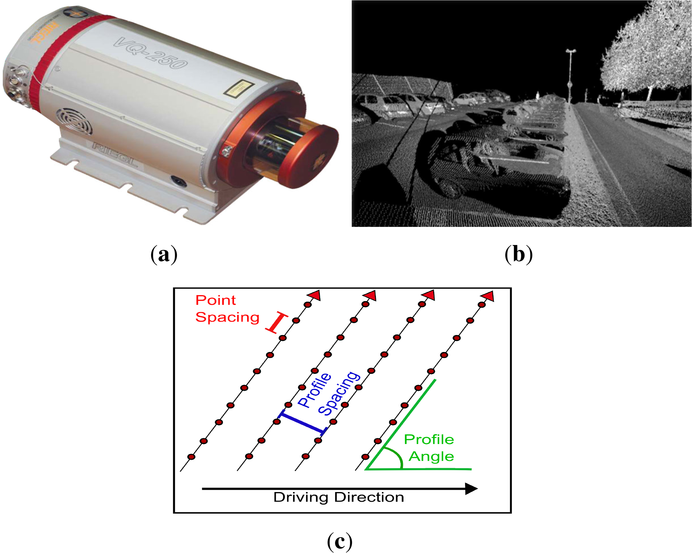
MOBILE Mapping Systems (MMSs) combine navigation and spatial measurement sensors on a moving platform. The spatial measurements can be captured by either cameras or laser scanners, and in both cases MMSs are capable of capturing high density spatial data accurately and efficiently. A single hi-end scanner similar to that displayed in Figure 1a, such as the Riegl VQ-450 [1], is capable of a pulse repetition rate of 550 kHz and produces high density point clouds (Figure 1b). Data volumes can increase rapidly, since many commercial MMSs such as the Optech Lynx [2], Trimble MX8 [3] or StreetMapper from 3D Laser Mapping [4] are dual scanner systems, although the MX8 and StreetMapper have both incorporated Riegl laser scanners.
As a relatively modern survey technology, assessing the performance of these systems and defining a survey specification that does not stipulate excessively prescriptive point density requirements is a complicated process. This is illustrated by the variety of methods proposed for specifying point density in survey specifications [5–7]. A method for accurately and rapidly quantifying point density for generic targets and MMSs is required to assist in this process, and this method would also assist with MMS design and MMS benchmarking. An MMS operator may not require two scanners capable of operating at 500 kHz if it can be demonstrated that two lower-specification scanners operating at 300 kHz are capable of achieving a suitable point density. Advances in this area can potentially provide MMS operators with savings in scan hardware, data storage and processing time.
Further research in this area will also assist the development of automatic algorithms. Automating the recognition of features in LiDAR point clouds is an ongoing research problem [8–13]. One of the limiting factors of these algorithms is the number of laser pulses striking and returning from the target per unit of area. This is because a target with few returns will be a more difficult test for an automated algorithm than one that is clearly defined. For example, algorithms documented by [14–17] require a minimum number of points or a minimum spacing between scan lines on cylindrical objects to recognise those features. Algorithms designed to identify road edges or road roughness for single scanner systems are particularly reliant on a suitable point density, because these systems do not have a second scanner to cover the road edge on the other side of the road. In [18], the authors quantified a point density threshold below which automated extraction algorithms were not reliable. A tool for assessing point density can be used to tailor these algorithms to commercial systems, or to tailor the survey to the algorithm (i.e., maintaining a certain point density). The importance of LiDAR point density was demonstrated for aerial LiDAR data in [19] where the point density, although algorithm dependent, directly impacted on the accuracy of the resulting models. In this paper we will present the innovative methodology developed at the NCG for determining MMS point density.
2. Background and Related Work
The number of laser returns per unit area is generally referred to as the point density. The number of points that strike a target (and therefore lead to a laser return) is predominantly influenced by the scanner hardware, the range to target and the target size. In their work on aerial and terrestrial LiDAR, the authors in [20] discuss point density, ways to define it for 3D data captured by multiple platforms and also the importance of point density during data processing. Assessing MMS performance has been approached using different methods, such as manufacturer hardware specifications [1], manual measurements using real-world MMSs [21,22] (although system and target-specific, this method has been advanced by benchmarking multiple mobile mapping systems [23]) or through LiDAR simulations. LiDAR simulations [24–26] are extremely useful for creating simulated datasets to inspect point clouds or test algorithms, but similar to the manual survey approach, they do not provide a capability for calculating point density. The importance of providing MMS operators with a method for calculating point density is recognised by manufacturers and the research community. Riegl supply a basic tool [27] with their RiACQUIRE software and other geometric formulae applied by [28,29] allow MMS operators to get a general idea of point density in certain areas, but none of these methods have included all of the required hardware and target parameters. The methodology we presented in [30] was the first to incorporate additional parameters such as target rotations, scanner rotations, changes in target height and changes in scanner height in calculating the position that each laser pulse should strike a surface. Scenario-specific parameters, such as multiple returns from a single laser pulse, occlusions or the laser footprint, are not modelled in MIMIC. Although these factors may change the position or number of individual laser pulses, the purpose of MIMIC is to provide a tool for assessing MMS hardware configurations during the mission planning stage, during algorithm development or during MMS benchmarking. Using this body of work, we have been able to extend our methodology for calculating point and profile distribution at a single target location and developed a method to combine these outputs into a measure of point density for entire targets and non-planar surfaces.
3. MIMIC
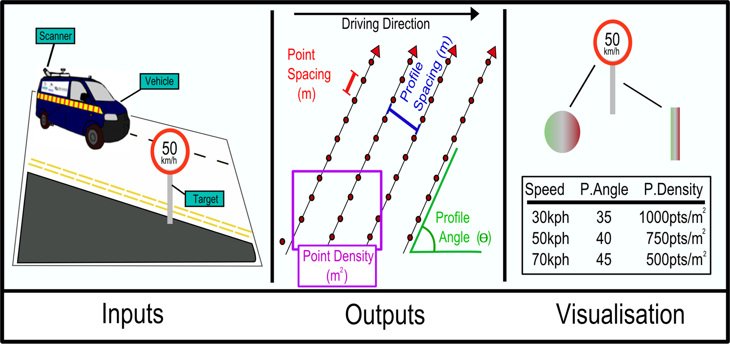
A prototype system called the “MobIle Mapping point densIty Calculator” or “MIMIC” has been designed and developed at the NCG. MIMIC is an innovative system for calculating point density. MIMIC and the multiple variables that need to be considered when designing a system to calculate point density were first introduced in [31]. MIMIC is compatible with different scanner hardware, scanner configuration, vehicle and target variables and its workflow comprises three main stages: variable input, point and profile calculation and visualisation, as illustrated in Figure 2.
3.1. Target Types
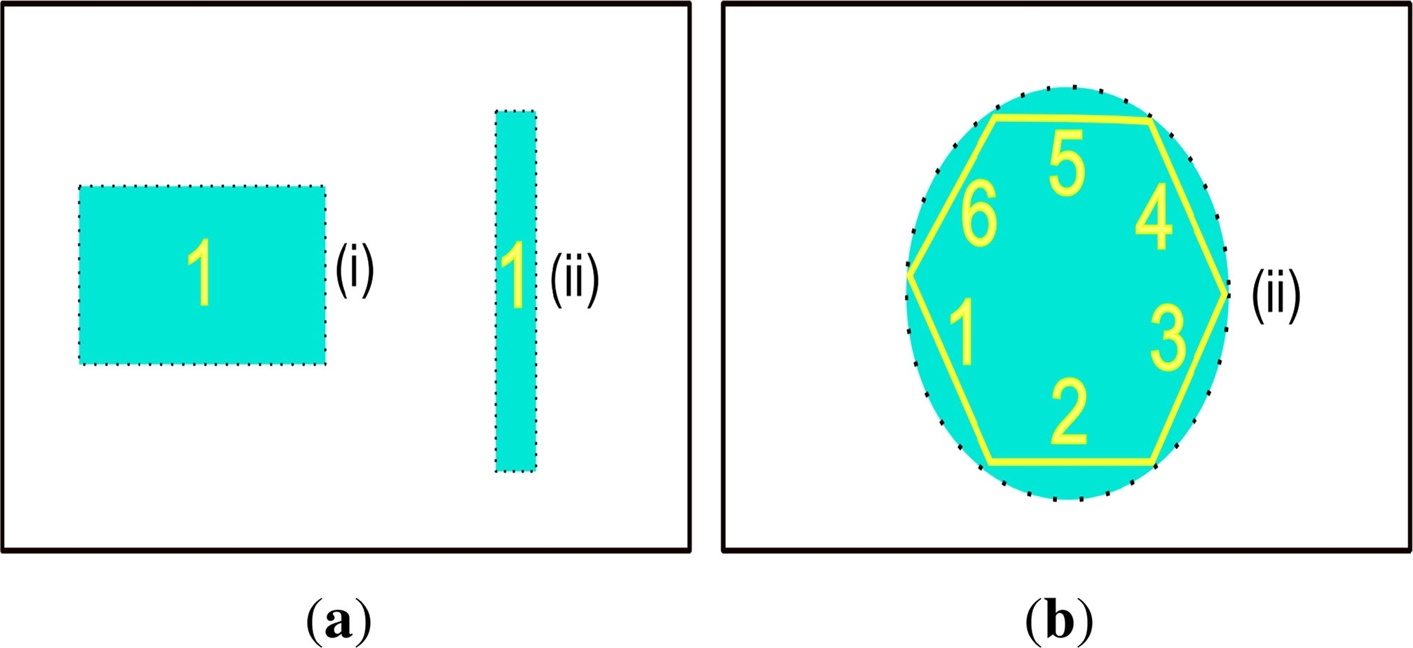
MIMIC requires 2D primitives such as those illustrated in Figure 3a as valid target types. To simplify the point density calculations, MIMIC applies rotation matrices, 3D surface normals and 2D geometrical formulae to these planar targets. For example, in
3.2. Applying a Grid Structure to Targets
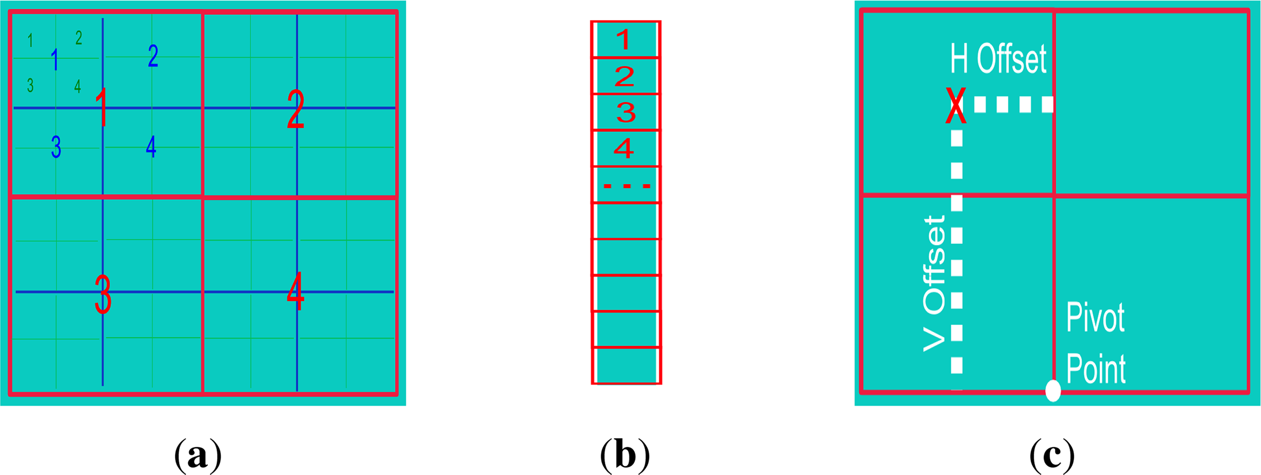
One of the shortcomings of existing calculation methods is that point spacing is only calculated at a single, central, target location. This influences the accuracy of the point density calculation, particularly when any rotation of the target results in a wide variation in point spacing across the target. To improve on this, MIMIC applies a grid structure to the target and the point spacing is then calculated for each grid cell centre. The number of cells in the grid structure is user-specified at the input stage when defining the target. MIMIC currently operates a 4-cells grid (2 × 2), a 16-cells grid (4 × 4) and a 64-cells grid (8 × 8), as illustrated in Figure 4a. Narrow vertical structures require a different grid structure than that displayed in Figure 4a. A single column grid structure is applied to narrow targets, as illustrated in Figure 4b. A 4 × 4 grid structure was applied for the standard target point density tests in this paper because it provided higher level of detail than the 1 × 1 or 2 × 2 grid structure. Additionally, because validation required manual measurements of the point cloud, the 4 × 4 grid structure was less time consuming than the 8 × 8 grid structure. For the same reason, a 6 × 1 grid structure was applied for the cylindrical targets.
3.3. Incorporating Target Rotations
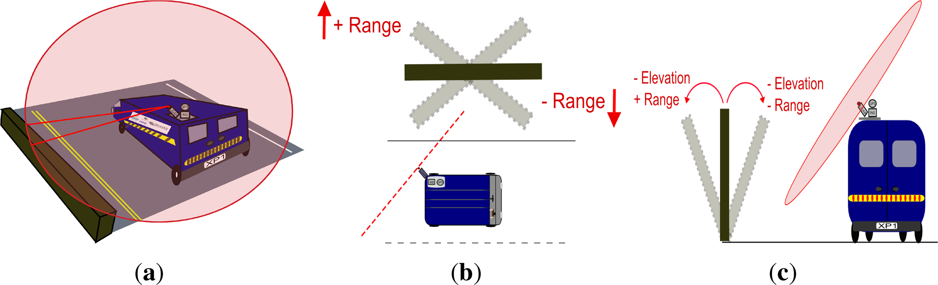
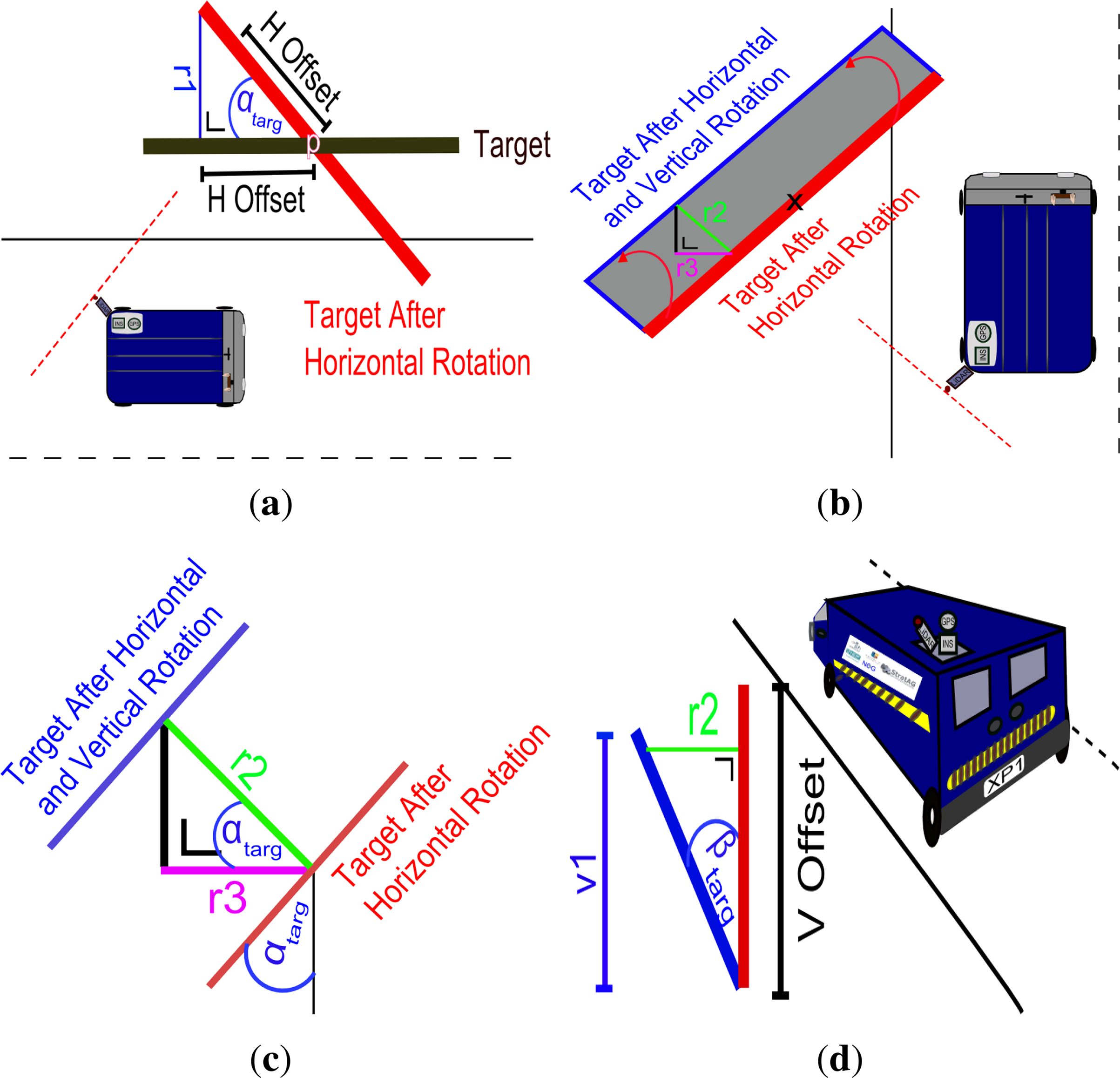
Rotations of the target alter the height of, and the range to, each grid cell centre in relation to the laser scanner on the MMS. MIMIC models this change by rotating the target around a central pivot point and tracking the resulting position of the grid cell centre. The position of each grid cell centre is calculated using the horizontal and vertical offsets illustrated in Figure 4c. The effect of target rotations on the range to the grid cell centre is dependent on what target rotations are applied and also the scanner orientation (Figure 5a). In Figure 5b a horizontal rotation of the target is illustrated. This type of target rotation can decrease or increase the range to alternate sides of the target. The elevation of the grid cell centres is not affected by a horizontal rotation of the target. Figure 5c illustrates a vertical rotation of the target. A target can incline away from, or towards, the MMS. If the target is inclined away from the MMS, the elevation of the grid cell centres decreases, but the range to each cell centre will increase. If the target is inclined towards the MMS, the elevation decreases and the range to the target will also decrease. Calculating the location of each grid cell centre is important for modelling variations in point spacing on a target and therefore point density. The following principles are applied to calculate the change in range to, and elevation of, each grid cell centre that results from a horizontal or vertical target rotation.
MIMIC initially calculates the change in range resulting from a horizontal rotation of the target. A horizontal rotation (αtarg) is applied to the target at the pivot point, p, as illustrated in Figure 6a. For each grid cell centre, the change in the horizontal range to the point, r1, can be calculated with
The range to each grid cell has now been amended to include horizontal and vertical target rotations. Figure 6d also illustrates the variables required for calculating the final elevation of each grid cell centre after a vertical rotation of the target. The amended elevation for each grid cell centre, v1, is calculated using
3.4. Calculating Point Density
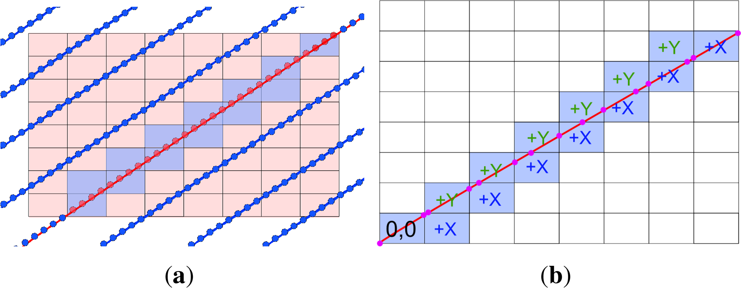
The amended elevations of, and horizontal ranges to, each grid cell centre are then included in the point spacing calculation for each grid cell centre. The methods employed by MIMIC for calculating point distribution were detailed and validated in [30]. However, to compute the point density of an entire target, the profile angle and profile spacing are combined with the point spacing that has been calculated for each grid cell centre. This is carried out by tracing each scan profile through the grid structure. Figure 7a illustrates this process. Starting at the bottom left hand corner of the target (0,0), MIMIC records the grid cells that each scan profile intersects. The length of the scan profile within that cell is recorded and the next grid cell is calculated, as Figure 7b illustrates. To calculate the number of points in that grid cell, the segment length is multiplied by the point spacing calculated for that grid cell. Using the computed horizontal and vertical profile spacing calculated by the method demonstrated in [30], each of the scan profiles that intersect the target can be modelled by incrementing the starting point (0,0) by the horizontal and vertical profile spacing.
3.5. Visualising MIMIC’s Outputs
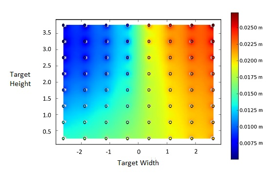
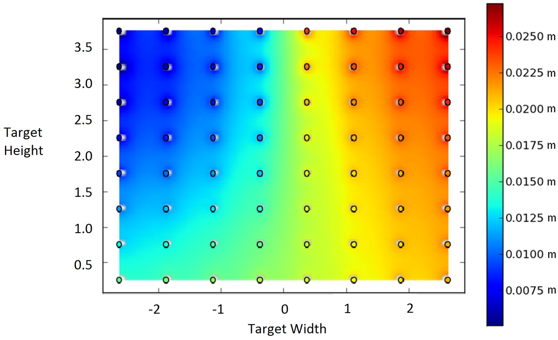
The visualisation module enables presentation of the information on profile angle, profile spacing, point spacing and point density to the user in a clear and easily understandable format. For example, using a form of interpolation known as Inverse Distance Weighting (IDW) [32], point information can be visualised. An example of this is illustrated in Figure 8, where point spacing has been calculated for a target that is 5 m wide and 4 m high on a planar surface for a single scanner system. The target range was 5 m and the target was rotated 30° in the horizontal plane. An 8 × 8 grid cell structure was applied. This method effectively visualises the point spacing and demonstrates the non-uniform distribution of point spacing on a rotated target.
4. Validating MIMIC’s Calculation Module
The capabilities of MIMIC were verified using point cloud data from two MMSs: the XP1 and the Optech Lynx. These datasets were used to experimentally verify that the point spacing, profile spacing and profile angle outputs from [30] could be combined into an accurate representation of the point density of a target. By varying the Mf and the PRR, MIMIC’s point density calculations for different scanners on angled and cylindrical targets were robustly tested. Data from the Optech Lynx was also used to verify calculations for dual scanner MMSs.
4.1. XP1
The multi-disciplinary research group StratAG, established to research advanced geotechnologies at NUI Maynooth, has designed and developed a multi-purpose land-based Mobile Mapping System, the XP1. The primary components of the XP1 are an IXSEA LANDINS GPS/INS, a Riegl VQ-250 300 kHz laser scanner and an imaging system consisting of up to six progressive-scan cameras. Imaging sensors include a FLIR thermal (un-cooled) SC-660 camera and an innovative 5-CCD multi-spectral camera capable of sensing across blue, green, red and two infra-red bandwidths. Unlike commercial systems, the XP1 is a single scanner system; however, even with a single Riegl VQ-250, the XP1 is capable of capturing dense point clouds. Additional information on the hardware configuration of the XP1 is available in our previous work investigating point and profile spacing [30,33–35].
4.2. Optech Lynx
The commercial system was the Optech Lynx M1 [2], which provided the opportunity for further validation with different scan hardware and a different system configuration. Unlike the XP1, the Optech Lynx M1 was a dual scanner MMS. Each full circle 2D scanner was capable of a 500 kHz PRR and a 200 Hz Mf. Additional data from the Optech Lynx data facilitated system verification in a number of ways. Firstly, the Optech Lynx was a dual scanner system and this was used to verify that MIMIC can cater for dual scanner MMSs. The variations in scanner orientation between the Optech Lynx and the XP1 further verified MIMIC’s profile calculations for different system configurations. Finally, the Optech M1 scanner was capable of operating at a higher Mf than the Riegl VQ-250 onboard the XP1, providing further test data for the profile calculations. Data from the Optech Linx M1 was also applied in the validation tests in [30] to validate point and profile spacing.
4.3. Target Selection for Validation
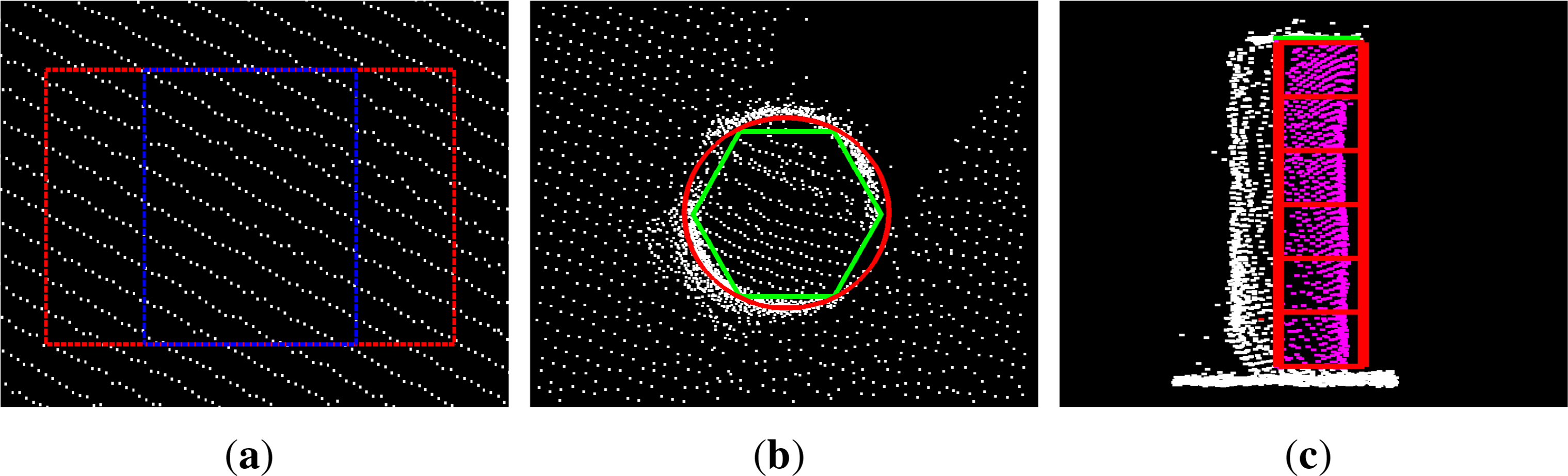
For each MMS dataset, a number of suitable areas for tests were identified and a series of sample measurements were recorded at each location. Using software designed by researchers at the NCG [36,37], areas consisting of suitable man-made vertical structures (e.g., walls, buildings, roofs, road-side infrastructure) were quickly identified and the XP1 survey data was extracted from large files of both rural and urban environments in Ireland. Optech Inc. supplied researchers at the NCG with survey data captured in the vicinity of their offices in Ontario. In each test area the point density was manually measured for a target and then compared with the calculated values from MIMIC. Figure 9a illustrates a selection of walls chosen to represent two types of planar target. Figure 9b illustrates a hexagonal approximation being applied to a cylinder and in Figure 9c the 6 × 1 grid structure is overlaid on one hexagonal face while the points are selected in each grid for manual verification.
5. Results and Discussion
The measured number of points striking a target was compared with MIMIC’s predicted values for a selection of angled and cylindrical targets for both single scanner and dual scanner MMS. The point density calculations were then further validated by gridding a target and comparing the number of points in each cell with MIMIC’s calculated value for that cell.
5.1. Point Density—Single Scanner
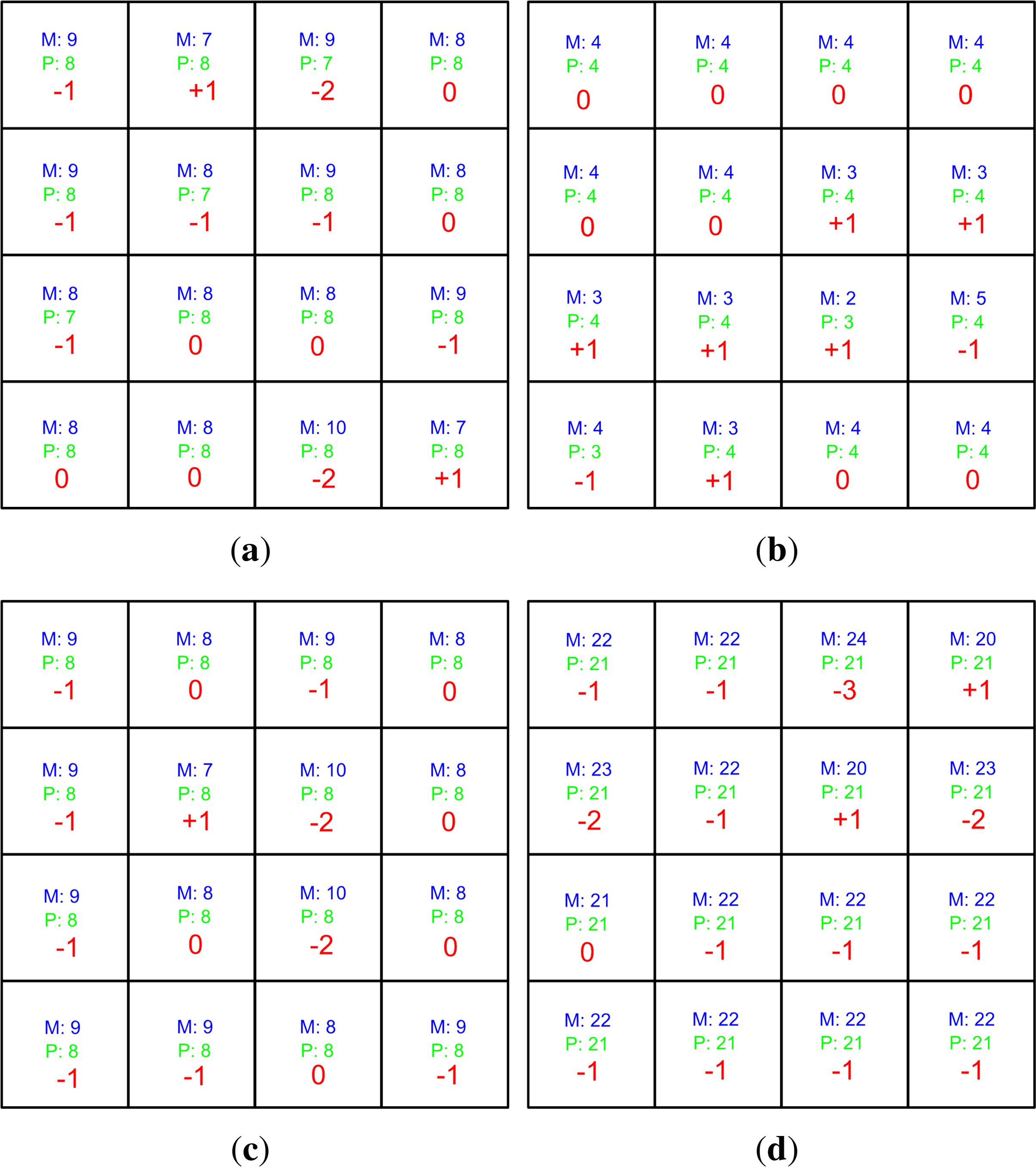
Four angled targets of dimensions 0.5 m × 0.5 m were identified in the point cloud and a 4 × 4 grid structure was applied to each to assess MIMIC’s performance for single scanner MMSs. The dimensions, orientation and range to each target were measured in the point cloud and then defined in MIMIC. Table 1 details the test parameters and scanner settings. MIMIC calculated total point density for the entire target and also calculated the point density for each grid cell. The point density was then calculated for the entire target and also for each individual grid cell, and compared with the measured values. The results in Table 2 demonstrate that MIMIC is capable of calculating the number of points on different targets for different scanner settings and vehicle velocities. Although there are errors in each case and MIMIC consistently underestimates the number of points that are striking the target, the errors must be evaluated with consideration of the number of profiles. The maximum error was on Target 3 in Table 2, in which it was underestimated by 23 points. Since it comprised 14 profiles, this translates into an error of approximately 1.64 points per profile.
To further investigate MIMIC’s point density calculations, the individual grid cells were examined. Targets 1–4 are illustrated in Figure 10. The greatest error on the 0.5 m × 0.5 m targets was an underestimation of 3 points for a grid cell on Target 4. This target exhibited the highest errors but it had approximately six times as many points per grid cell as Target 2, which was the most accurate calculation with an error of only 6.5% for the entire target. The point density for Target 2 was correctly predicted for eight (50%) of the grid cells. The remaining grid cells were low overestimates or underestimates of 1 point. Overall, the errors were low, particularly when compared with the number of points per profile. The average error for all of the targets was just 0.88 points per profile.
5.2. Point Density—Dual Scanner
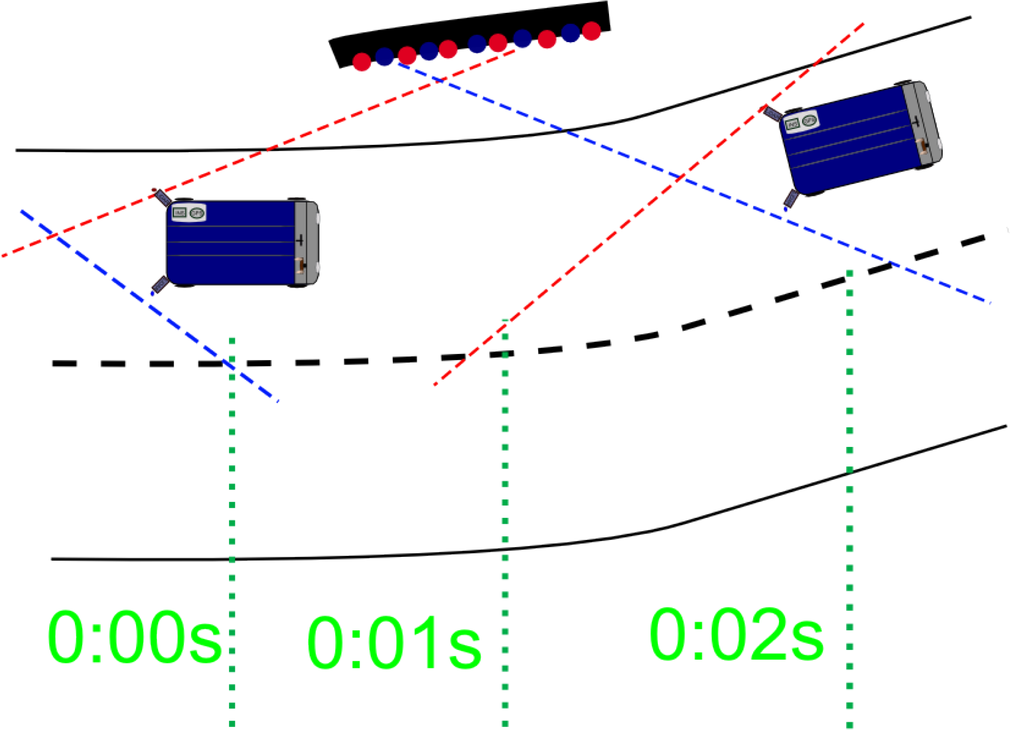
One potential error source is that MIMIC assumes zero course deviation and therefore does not calculate a separate target orientation in relation to Scanner 2. Figure 11 illustrates this potential error source. Laser pulses from Scanner 1 first strike the target at time = 0 seconds, but Scanner 2 cannot survey the target at this time due to its orientation. The pulses from Scanner 2 first strike the object 2 seconds later, but by this time the heading of the vehicle has changed as it travels around a curve. This heading change has altered the orientation of the target in relation to Scanner 2, whereas MIMIC applies the original target orientation specified by the user. Any changes in heading, orientation, scanner height, vehicle velocity or the accuracy of the MMS positioning solution between the two measurement times will result in errors when verifying MIMIC’s calculations.
For example, in the angled surface tests on Target 1, a difference of approximately 2 seconds exists between the measurements recorded on the target by Scanner 1 and those recorded by Scanner 2. The GPS time was 139,340.636 seconds for the first pulse striking the target from Scanner 1 and 139,342.604 for the first pulse striking the target from Scanner 2. The point density calculation was influenced by this in a number of ways:
Heading: There was a course deviation of 2.996° between the two measurements. This introduced errors into the profile angle, profile spacing and point spacing calculations for Scanner 2.
Range: This resulted in a change in horizontal range to the target of 0.4 m. This introduced errors into the point spacing calculations.
Elevation: There was a 0.18 m height change in this time that was not factored into the calculation. This introduced errors into the point spacing calculations.
Positioning: Any errors in positioning (i.e., loss of GNSS signal) that might arise during this period will also influence the point distribution and absolute accuracy of the target surface in the point cloud.
The Optech Lynx data was used to verify MIMIC’s calculations for a dual scanner system. Table 3 provides details on the four targets. Targets of two different dimensions were chosen. A comparison of the manually measured points and MIMIC’s calculated values are detailed in Table 4. In each case the percent error for Scanner 1 was within 6% of Scanner 2. Except Target 4, in all other cases MIMIC underestimated the point density of the target. The largest errors existed for Target 2, however both scanners were displaying large errors, which implied there was a problem with that target in the point cloud.
The scanner offset increases the horizontal range to the target from Scanner 2, which results in a lower point density than for Scanner 1. For example, the predicted point density on Target 1 is over 100% higher for Scanner 1 than for Scanner 2. Additionally, the orientation of Scanner 2 also influences the point density on targets rotated towards the MMS. This was not a constant effect, as the opposite was the case for Targets 3 and 4 where the negative rotation of the target results in an increased point spacing and profile spacing for Scanner 1 but a decreased point spacing and profile spacing for Scanner 2. This resulted in an increase in point density for Scanner 2 relative to Scanner 1. Scanner 2 captures 6% more points than Scanner 1 for Target 4. Potential course changes can be implemented as future work but for the current objectives of MIMIC the results have shown that it can operate without them. A maximum difference of 6.02% error when comparing the point density from Scanner 1 to that of Scanner 2 demonstrates that MIMIC can robustly calculate point density for dual scanner MMSs in situations where small course deviations are present.
5.3. Point Density—Cylindrical Targets
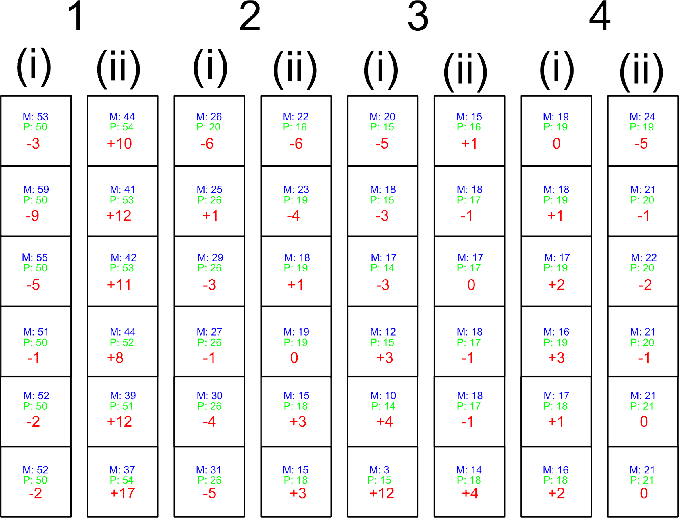
For these tests, 3D cylindrical targets were converted into a series of narrow vertical 2D planes and surveyed using a single scanner MMS. Therefore only 2 of the cylinder’s “faces” were surveyed. Figure 9b illustrates the process of applying a hexagonal planar shape to identify each face of the cylindrical target from top and side view. This manual classification process potentially introduces errors. These faces were denoted (i) and (ii) and corresponded to a manual interpretation of the “faces” of the cylinder. Each cylinder therefore consisted of two planes, with different orientations. These orientations are listed in Table 5. Figure 9c illustrates the process of gridding a vertical target and measuring the points in that grid cell. The calculated point density was compared with the manual measurement for each cylinder face.
The results displayed in Table 5 show that the percent error has increased for cylindrical targets. These results reinforce the hypothesis that the manual interpretation of each cylinder face could potentially result in points being incorrectly assigned to a face. For each target, an underestimation of point density on one cylinder face has been matched with an overestimation of point density on the other. The point density for the combined cylinder was calculated and the results are displayed in Table 6. For each cylinder as a whole, the point density errors were less than 10%. The predicted and measured values for each grid cell are displayed for both faces of all 4 cylinders in Figure 12. The Face (ii) of Cylinder 1 had the highest error of 27.2%. However, the percent error for this entire cylinder was only −8.2% as displayed in Table 6. This 19% reduction in percent error suggests an incorrect manual classification of the Faces (i) and (ii) of Cylinder 1. The base of Cylinder 3, Face (i) was obstructed by vegetation, and the magnitude of the error reflects this with MIMIC overestimating by 12 points in this grid cell alone. MIMIC does not model obstructions between the scanner and the target. Overall, the results were encouraging. Excluding Cylinder 1, Face (ii), the percent errors in Table 5 for each target are comparable with the percent error for the planar targets in Table 2. Table 7 lists the error per profile for each target face. The highest error was 2.2 points per profile on Cylinder 1, Face (ii), but this has already been shown to contain large errors in point density. The average error per profile was 0.51 point, an improvement on the previous tests with the planar targets. These tests validate MIMIC’s method of approximating curved cylindrical targets with a combination of planar targets.
5.4. Contribution of Errors
A series of tests are designed to demonstrate how the errors in the calculation of the output values (i.e., profile angle, profile spacing and point spacing) affect the point density calculation. The greatest error in the output values detailed in [30] was approximately 5% of the true value. Each output value was therefore modified by ±5%, and the point density was then re-calculated for a target. The effect of the ±5% error on the final point density calculation was then identified. A parallel, vertical target (1 m × 0.5 m) was specified at a range of 6 m from the scanner. The scanner defined in MIMIC was the XP1’s VQ250, orientated at 45°/45° and operating at a 300 kHz PRR and a 100 Hz Mf. The vehicle velocity was simulated at 50 km/h. Table 8 details the results of these tests. Errors in the profile angle calculation have the biggest impact on the point density calculation. A −5% error in the profile angle calculation results in a 12.23% error in the point density calculation, whereas a +5% error in the profile angle calculation results in an 8.9% error in the point density calculation. Interestingly, a ±5% error in the profile spacing calculation has very little effect on the point density calculation, less than 1%. Comparing these values with the previous results for point density on angled vertical surfaces, cylinders and irregular surfaces, it is possible to see how a small error in calculating profile angle, profile spacing or point spacing could explain the errors that are present.
6. Conclusions
This paper presented MIMIC as a method to calculate point density using the outputs of profile angle, profile spacing and point spacing. A gridding approach was developed to accurately calculate point spacing on large or angled targets. A 4 × 4 grid structure was chosen as the most suitable for these tests because it was capable of accurately calculating point density while also minimising the manual component of the validation tests. MIMIC was validated using a combination of targets. Point density was calculated for planar targets and a hexagonal planar approximation of a cylinder was applied to facilitate calculations on a curved surface. Variations in the target dimensions, orientation, elevation and range robustly tested MIMIC’s point density calculations using different scanner parameters. MIMIC’s point density calculations were also validated for a dual scanner MMS. An average error of less than one point per profile validated MIMIC’s point density calculations for angled planar targets. The second target type was a multi-faced cylindrical target and the highest errors were returned when calculating point density for this target type. This was potentially due to manual interpretation of each face on the cylinder or obstructions between the scanner and the target. After combining the two faces, an average error of less than one point per profile validated MIMIC’s point density calculations for cylindrical targets. Once the point density calculation for a single scanner system was validated, the ability of MIMIC to calculate point density resulting from a change in the scanner position and orientation was tested. MIMIC’s point density calculations were then validated using a dual scanner MMS. Scanner 2 results in approximately 50% lower point density than Scanner 1. This value is dependent on the target orientation, the range to the target and the orientation of the target. MIMIC calculated point density on a cylindrical target, and although errors were present when individual faces were examined, the total point density of the cylinder results in errors ≤ 4%, validating MIMIC’s methodology of calculating point density for dual scanner system on cylindrical targets. For both angled and cylindrical targets, similar point density percent errors for Scanner 1 and Scanner 2 imply that MIMIC can calculate point density accurately without incorporating course deviation.
Acknowledgments
Research presented in this paper was funded by the Irish Research Council (IRC) and the Enterprise Partner, Pavement Management Services Ltd., by the NRA research fellowship program, ERA-NET SR01 projects and by a Strategic Research Cluster grant (07/SRC/I1168) from Science Foundation Ireland under the National Development Plan. The authors would also like to thank Optech Inc. for supplying additional test data.
Author Contributions
MIMIC was developed by Conor Cahalane. Conor P. McElhinney and Paul Lewis collaborated with Conor Cahalane in designing the procedures for experimental validation. Tim McCarthy designed and developed the XP1, used in validation, and provided technical advice at all stages. All authors contributed equally in preparing this manuscript.
Conflicts of Interest
The authors declare no conflict of interest.
References
- Riegl. Dual Scanner Data sheet Riegl VMX-450. Available online: http://www.riegl.com/ncproducts/mobile-scanning/produktdetail/product/scannersystem/10/ (accessed on 9 October 2012).
- Optech. Optech Lynx M1 and V200 System Specifications. Available online: http://www.optech.ca/lynx.htm (accessed on 9 October 2012).
- Trimble. Trimble MX8 Mobile Mapping System. Available online: http://www.trimble.com/geospatial/Trimble-MX8.aspx?dtID=overview (accessed on 9 October 2012).
- 3D Laser Mapping, StreetMapper Technical Report. Available online: http://www.3dlasermapping.com/downloads/brochures (accessed on 5 October 2012).
- Yen, W.; Ravani, B; Lasky, T. LiDAR for Data Efficiency. Available online: http://www.wsdot.wa.gov/Research/Reports/700/778.1.htm (accessed on 5 October 2011).
- Florida Department of Transport. Terrestrial Mobile LiDAR Surveying and Mapping Guidelines. Available online: http://www.dot.state.fl.us/surveyingandmapping/regulations.shtm (accessed on 5 October 2012).
- Olsen, M.J; Roe, G.; Glennie, C.; Persi, F.; Reedy, M.; Hurwitz, D.; Williams, K.; Tuss, H.; Squellati, A.; Knodler, M. NCHRP 15–44 Guidelines for the Use of Mobile LiDAR in Transportation Applications, 2013. Available online: http://apps.trb.org/cmsfeed/TRBNetProjectDisplay.asp?ProjectID=2972 (accessed on 3 April 2013).
- Becker, S.; Haala, N. Grammar supported facade reconstruction from mobile lidar mapping. Int. Arc. Photogramm. Remote Sens 2009, 38, 229–234. [Google Scholar]
- Hammoudi, K.; Dornaika, F.; Paparoditis, N. Extracting building footprints from 3D point clouds using terrestrial laser scanning at street level. Int. Arch. Photogramm. Remote Sens. Spat. Sci. Inf 2009, 38, 65–70. [Google Scholar]
- McElhinney, C.P; Kumar, P.; Cahalane, C; McCarthy, T. Initial results from European Road Safety Inspection (EURSI) mobile mapping project. Int. Arch. Photogramm. Remote Sens. Spat. Inf. Sci 2010, 38, 440–445. [Google Scholar]
- Kumar, P.; McElhinney, C.P; Lewis, P.; McCarthy, T. Automated road markings extraction from mobile laser scanning data. Int. J. Appl. Earth Obs. Geoinf 2014, 32, 125–137. [Google Scholar]
- Pu, S.; Vosselman, G. Extracting windows from terrestrial laser scanning. Int. Arch. Photogramm. Remote Sens. Spat. Inf. Sci 2007, 36, 320–325. [Google Scholar]
- Pu, S.; Rutzinger, M.; Vosselman, G.; Elberink, S. Recognizing basic structures from mobile laser scanning data for road inventory studies. ISPRS J. Photogramm. Remote Sens 2011, 66, 28–39. [Google Scholar]
- Brenner, C. Global localization of vehicles using local pole patterns. Lect. Note Comput. Sci 2009, 5748, 61–70. [Google Scholar]
- Kukko, A.; Jaakola, A.; Lehtomäki, M.; Kaartinen, H.; Chen, Y. Mobile mapping system and computing methods for modelling of road environment. In Proceedings of 2009 Joint Urban Remote Sensing Event, Shanghai, China, 20–22 May 2009; pp. 1–6.
- Lehtomäki, M.; Jaakkola, A.; Hyyppä, J.; Kukko, A.; Kaartinen, H. Detection of vertical pole-like objects in a road environment using vehicle-based laser scanning data. Remote Sens 2010, 2, 331–336. [Google Scholar]
- Wu, B.; Yu, B.; Yue, W.; Shu, S.; Tan, W.; Hu, C.; Huang, Y.; Wu, J.; Liu, H. A voxel based-method for automated identification and morphological parameters estimation of individual street trees from mobile laser scanning data. Remote Sens 2013, 5, 584–611. [Google Scholar]
- Kumar, P.; McElhinney, C.P; Lewis, P.; McCarthy, T. An automated algorithm for extracting road edges from terrestrial mobile LiDAR data. ISPRS J. Photogramm. Remote. Sens 2013, 85, 44–55. [Google Scholar]
- Kaartinen, H.; Hyyppä, J.; Gulch, E.; Vosselman, G.; Hyyppä, H.; Matikainen, L.; Hofmann, A.D.; Mäder, U.; Persson, Å.; Söderman, U.; et al. Accuracy of 3D city models : EuroSDR comparison. Int. Arch. Photogramm. Remote Sens. Spat. Inf. Sci 2005, 36, 227–232. [Google Scholar]
- Lari, Z.; Habib, A. Alternative methodologies for the estimation of local point density index: Moving towards adaptive LiDAR data processing. Int. Arch. Photogramm. Remote Sens. Spat. Inf. Sci 2012, 39, 127–132. [Google Scholar]
- Kukko, A.; Andrei, C.O.; Salminen, V.M.; Kaartinen, H.; Chen, Y.; Rönnholm, P.; Hyyppä, H.; Hyyppä, J.; Chen, R.; Haggrén, H.; et al. Road environment mapping system of the Finnish Geodetic Institute-FGI Roamer. Int. Arch. Photogramm. Remote Sens. Spat. Inf. Sci 2007, 36, 241–247. [Google Scholar]
- Hesse, C.; Kutterer, H. A mobile mapping system using kinematic terrestrial laser scanning (KTLS) for image acquisition. In Proceedings of 2007 the 8th Conference on Optical 3-D Measurement Techniques, Zurich, Switzerland, 9–13 July 2007; pp. 134–141.
- Lin, Y.; Hyyppä, J.; Kaartinen, H.; Kukko, A. Performance analysis of mobile laser scanning systems in target represenation. Remote Sens 2013, 5, 3140–3155. [Google Scholar]
- Kukko, A.; Hyyppä, J. Small-footprint laser scanning simulator for system validation, error assessment and algorithm development. Photogramm. Eng. Remote Sens 2009, 75, 1177–1189. [Google Scholar]
- Lohani, B.; Mishra, R. Generating LiDAR data in laboratory: LiDAR simulator. Int. Arch. Photogramm. Remote Sens. Spat. Inf. Sci 2007, 52, 12–14. [Google Scholar]
- Yoo, H.; Goulette, F.; Senpauroca, J.; Lepere, G. Simulation based comparative analysis for the design of laser terrestrial mobile mapping. In Proceedings of 2009 the 6th International Symposium on Mobile Mapping Technology, Sao Paolo, Brazil, 21–24 July 2009; pp. 839–854.
- Riegl. RiACQUIRE Software Datasheet. Available online: http://products.rieglusa.com/item/software-packages/riacquire-data-acquisition-software/item-1011 (accessed on 11 October 2012).
- Puente, I.; Gonzalez-Jorge, H.; Martinez-Sanchez, J.; Arias, P. Review of mobile mapping and surveying technologies. Measurement 2013, 46, 2128–2144. [Google Scholar]
- Hofmann, S.; Brenner, C. Quality assessment of automatically generated feature maps for future driver assistance systems. In Proceedings of 2009 the 17th ACM SIGSPATIAL International Conference on Advances in Geographic Information Systems, New York, NY, USA, 4–6 November 2009; pp. 500–503.
- Cahalane, C.; McElhinney, C.P.; Lewis, P.; McCarthy, T. Calculation of target-specific point distribution for 2D mobile laser scanners. Sensors 2014, 14, 9471–9488. [Google Scholar]
- Cahalane, C.; McElhinney, C.P.; Lewis, P.; McCarthy, T. MIMIC: Mobile mapping point density calculator. In Proceedings of the 3rd International Conference on Computing for Geospatial Research and Applications, Washington, DC, USA, 1–3 July 2012.
- Shepard, D. A two-dimensional interpolation function for irregularly-spaced data. In Proceedings of 1968 the 23rd National Conference ACM, New York, NY, USA, 1968; pp. 517–524.
- Cahalane, C.; McElhinney, C.P.; McCarthy, T. Mobile mapping system performance: An analysis of the effect of laser scanner configuration and vehicle velocity on scan profiles. In Proceedings of 2010 the European LiDAR Mapping Forum, Hague, The Netherlands, 30 November–1 December 2010.
- Cahalane, C.; McElhinney, C.P.; McCarthy, T. Calculating the effect of dual-axis scanner rotations and surface orientation on scan profiles. In Proceedings of 2011 the 7th International Symposium on Mobile Mapping Technology, Krakaw, Poland, 13–16 June 2011.
- Cahalane, C.; McCarthy, T.; McElhinney, C.P. Mobile mapping system performance: An initial investigation into the effect of vehicle speed on laser scan lines. In Proceedings of 2010 the Remote Sensing and Photogrammety Society Annual Conference “From the Sea-Bed to the Cloudtops”, Cork, Ireland, 1–3 September 2010.
- Lewis, P.; McElhinney, C.P; McCarthy, T. Lidar data management pipeline; from spatial database population to web-application visualization. In Proceedings of the 3rd International Conference on Computing for Geospatial Research and Applications, Washington, DC, USA, 1–3 July 2012.
- McElhinney, C.P.; Lewis, P.; McCarthy, T. Mobile terrestrial LiDAR data-sets in a spatial database framework. In Proceedings of 2011 the 7th International Symposium on Mobile Mapping Technology, Krakaw, Poland, 13–16 June 2011.


| No. | Hr (m) | Vel (m/s) | Zdiff (m) | αtarg | PRR | Mf |
|---|---|---|---|---|---|---|
| 1 | 7.665 | 5.813 | 1.218 | 17.33° | 125 kHz | 100 Hz |
| 2 | 11.796 | 7.224 | 1.953 | −1.12° | 125 kHz | 100 Hz |
| 3 | 11.432 | 7.21 | 2.089 | 0.1° | 250 kHz | 150 Hz |
| 4 | 6.422 | 5.318 | 1.345 | 22.79° | 250 kHz | 150 Hz |
| No. | MIMIC | Measured | %Error | No. Profiles | Error Per profile |
|---|---|---|---|---|---|
| 1 | 127 pts | 137 pts | 7.3% | 14 | 0.7 pts |
| 2 | 58 pts | 62 pts | 6.5% | 9 | 0.4 pts |
| 3 | 124 pts | 147 pts | 15.6% | 14 | 1.64 pts |
| 4 | 337 pts | 352 pts | 4.3% | 22 | 0.68 pts |
| Target | Width (m) | Height (m) | αtarg | Hr (m) | Zdiff (m) |
|---|---|---|---|---|---|
| 1 | 1.0 | 0.5 | 16.53° | 8.736 | 0.859 |
| 2 | 0.5 | 0.5 | 16.53° | 8.736 | 0.859 |
| 3 | 1.0 | 0.5 | −25.14° | 5.756 | 2.018 |
| 4 | 0.5 | 0.5 | −25.14° | 5.756 | 2.018 |
| Target | Scanner | MIMIC | Measured | %Error |
|---|---|---|---|---|
| 1 | 1 | 385 pts | 415 pts | 7.2% |
| 1 | 2 | 190 pts | 219 pts | 13.2% |
| 2 | 1 | 193 pts | 226 pts | 14.6% |
| 2 | 2 | 96 pts | 116 pts | 17.2% |
| 3 | 1 | 388 pts | 417 pts | 6.9% |
| 3 | 2 | 432 pts | 444 pts | 2.7% |
| 4 | 1 | 193 pts | 194 pts | 0.5% |
| 4 | 2 | 216 pts | 207 pts | 4.3% |
| Target (Face) | Hr (m) | αtarg | MIMIC | Measured | %Error |
|---|---|---|---|---|---|
| 1(i) | 5.118 | 0.81° | 301 pts | 322 pts | −6.5% |
| 1(ii) | 5.118 | 49.35° | 313 pts | 246 pts | +27.2% |
| 2(i) | 6.692 | 29.12° | 150 pts | 150 pts | 0% |
| 2(ii) | 6.692 | 77.22° | 108 pts | 112 pts | −3.6% |
| 3(i) | 7.950 | 71.36° | 87 pts | 80 pts | +8.7% |
| 3(ii) | 7.950 | 19.71° | 101 pts | 104 pts | −2.8% |
| 4(i) | 7.438 | 66.81° | 111 pts | 101 pts | +9.9% |
| 4(ii) | 7.438 | 19.08° | 121 pts | 137 pts | −11.7% |
| Target | MIMIC | Measured | %Error |
|---|---|---|---|
| 1 | 614 | 568 | +8.0% |
| 2 | 258 | 262 | −1.5% |
| 3 | 188 | 205 | −8.2% |
| 4 | 232 | 238 | −2.5% |
| Target | Face | Profiles | Error | Error per profile |
|---|---|---|---|---|
| 1 | (i) | 28 | 21 pts | 0.75 pts |
| 1 | (ii) | 30 | 67 pts | 2.2 pts |
| 2 | (i) | 32 | 0 pts | 0.00 pts |
| 2 | (ii) | 32 | 4 pts | 0.12 pts |
| 3 | (i) | 34 | 7 pts | 0.20 pts |
| 3 | (ii) | 34 | 3 pts | 0.08 pts |
| 4 | (i) | 38 | 10 pts | 0.26 pts |
| 4 | (ii) | 38 | 16 pts | 0.42 pts |
| Input | %Variation | Amended | MIMIC | %Error |
|---|---|---|---|---|
| Profile Angle | +5% | 691 pts | 759 pts | 8.9% |
| Profile Angle | −5% | 852 pts | 759 pts | 12.2% |
| Profile Spacing | +5% | 756 pts | 759 pts | 0.4% |
| Profile Spacing | −5% | 763 pts | 759 pts | 0.5% |
| Point Spacing | +5% | 723 pts | 759 pts | 4.7% |
| Point Spacing | −5% | 799 pts | 759 pts | 5.3% |
© 2014 by the authors; licensee MDPI, Basel, Switzerland This article is an open access article distributed under the terms and conditions of the Creative Commons Attribution license (http://creativecommons.org/licenses/by/3.0/).
Share and Cite
Cahalane, C.; McElhinney, C.P.; Lewis, P.; McCarthy, T. MIMIC: An Innovative Methodology for Determining Mobile Laser Scanning System Point Density. Remote Sens. 2014, 6, 7857-7877. https://doi.org/10.3390/rs6097857
Cahalane C, McElhinney CP, Lewis P, McCarthy T. MIMIC: An Innovative Methodology for Determining Mobile Laser Scanning System Point Density. Remote Sensing. 2014; 6(9):7857-7877. https://doi.org/10.3390/rs6097857
Chicago/Turabian StyleCahalane, Conor, Conor P. McElhinney, Paul Lewis, and Timothy McCarthy. 2014. "MIMIC: An Innovative Methodology for Determining Mobile Laser Scanning System Point Density" Remote Sensing 6, no. 9: 7857-7877. https://doi.org/10.3390/rs6097857