Estimating Forest Aboveground Biomass by Combining ALOS PALSAR and WorldView-2 Data: A Case Study at Purple Mountain National Park, Nanjing, China

Abstract
: Enhanced methods are required for mapping the forest aboveground biomass (AGB) over a large area in Chinese forests. This study attempted to develop an improved approach to retrieving biomass by combining PALSAR (Phased Array type L-band Synthetic Aperture Radar) and WorldView-2 data. A total of 33 variables with potential correlations with forest biomass were extracted from the above data. However, these parameters had poor fits to the observed biomass. Accordingly, the synergies of several variables were explored to identify improved relationships with the AGB. Using principal component analysis and multivariate linear regression (MLR), the accuracies of the biomass estimates obtained using PALSAR and WorldView-2 data were improved to approximately 65% to 71%. In addition, using the additional dataset developed from the fusion of FBD (fine beam dual-polarization) and WorldView-2 data improved the performance to 79% with an RMSE (root mean square error) of 35.13 Mg/ha when using the MLR method. Moreover, a further improvement (R2 = 0.89, relative RMSE = 17.08%) was obtained by combining all the variables mentioned above. For the purpose of comparison with MLR, a neural network approach was also used to estimate the biomass. However, this approach did not produce significant improvements in the AGB estimates. Consequently, the final MLR model was recommended to map the AGB of the study area. Finally, analyses of estimated error in distinguishing forest types and vertical structures suggested that the RMSE decreases gradually from broad-leaved to coniferous to mixed forest. In terms of different vertical structures (VS), VS3 has a high error because the forest lacks undergrowth trees, while VS4 forest, which has approximately the same amounts of stems in each of the three DBH (diameter at breast height) classes (DBH > 20, 10 ≤ DBH ≤ 20, and DBH < 10 cm), has the lowest RMSE. This study demonstrates that the combination of PALSAR and WorldView-2 data is a promising approach to improve biomass estimation.
1. Introduction
Precise quantification of forest aboveground biomass (AGB) on a regional to global scale is of increasing importance in the context of reducing emissions from deforestation and forest degradation in developing countries (REDD+) and compliance with the Kyoto Protocol [1–3]. In a forest inventory, the sample plotting method provides very accurate AGB values at the plot level [4]. Due to the high cost of this traditional plot-based investigation for AGB and the difficulties of its implementation in remote areas, interest in the use of remotely sensed data acquired from spaceborne or airborne sensors to estimate forest AGB has increased in recent decades. Remote sensing provides a key source of data for updated, consistent, and spatially explicit assessment of forest biomass and its dynamics, particularly in large countries with limited accessibility [5,6].
Optical images have long been used to estimate forest parameters and assess wood biomass [7–9]. Estimating the AGB has been mainly achieved by using spectral reflectance and/or vegetation indices, such as the normalized difference vegetation index (NDVI), which is computed from the red and near-infrared (NIR) bands [10–12]. However, a major limitation of vegetation indices is that these indices reach a saturation level during the estimation of high-density biomass [13–15]. The saturation point varies greatly depending on the source data and the vegetation type and ranges from 15 to 100 Mg/ha for visible/NIR vegetation indices [11,16]. Other studies have also indicated that the NDVI approaches a saturation level when the vegetation age is greater than 15 years in tropical forests [8]. In addition, optical remote sensing provides limited information on the vertical distribution of forest structure [17], and compiling a temporally and radiometrically consistent cloud-free datasets over large areas is not always possible [6].
Over the past two decades, a large number of researchers have contributed to the study of the application of radar (Radio Detection and Ranging) for forestry [18,19]. Many studies have shown that forest biomass can be retrieved using SAR (Synthetic Aperture Radar) data because SAR can penetrate cloud and forest canopies [20–22]. The major advantage of all SAR systems is the weather- and daylight-independency of the system [20,23,24]. In addition, numerous studies have also reported that long-wavelength (e.g., L and P bands) SAR is more appropriate than short-wavelength (e.g., X and C bands) SAR for forest biomass estimations [25,26]. In this case, the detected radiation is mostly due to backscattering from the branches and stems of the trees, and thus L- and P-band SAR should respond characteristically to forest volume and biomass [22,27,28]. Additionally, long wavelength can travel without having a sight. The successful launch of ALOS (Advanced Land Observing Satellite) in 2006 increased the potential for the use of radar to measure AGB because PALSAR/ALOS is the first long-wavelength (L-band, 23-cm wavelength) SAR satellite sensor with the capability of collecting cross-polarized HV (horizontal-send, vertical-receive) and VH (vertical-send, horizontal-receive) data in addition to HH (horizontal-send, horizontal-receive) and VV (vertical-send, vertical-receive) data. Although the ALOS satellite stopped to operate in April 2011, the systematically collected PALSAR data from this satellite show great potential for AGB estimates on a large scale [25,29,30]. However, AGB estimation using the biomass-PALSAR backscattering relationship remains problematic due not only to the saturation at high biomass levels (i.e., the backscatter power no longer increases with AGB or volume) but also to the spatial heterogeneity of forests, which can generate unclear data [3,21,31].
Light detection and ranging (LiDAR) data can provide detailed vegetation structure measurements at discrete locations covering circular or elliptical footprints from a few centimeters to tens of meters in diameter [32,33]. LiDAR instruments mounted on airplanes emit active laser pulses and measure various echoes of the signal, resulting in accurate AGB estimations for various forests with no saturation at higher biomass levels [34–36]. However, LiDAR systems are often limited to airborne acquisition, which is better suited to providing samples (e.g., transects) rather than full wall-to-wall coverage over large areas [4,37,38]. Therefore, even though LiDAR provides the best estimates of forest biomass, observations over large areas remain problematic, making complete coverage at landscape and regional scales uncommon, with data costs often dictating government support for LiDAR or its inclusion in collection activities [39].
The globally and freely available Landsat TM (Thematic Mapper) and ETM+ (Enhanced Thematic Mapper Plus) data, which have a medium resolution (30 m for TM/ETM+ multispectral bands), have been widely used for mapping forest biomass on a regional to global scale in numerous studies [6,14,40,41]. However, the limited spatial detail misses small-scale biomass variability. In recent years, the successful launch of a number of commercial satellites with high resolution from tens of centimeters to a few meters (e.g., IKONOS, QuickBird, SPOT5, GeoEye-1, WordView-1&2) has provided an approach to this problem. The WorldView-2, launched in October 2009, acquires data with more multispectral bands (eight bands) and higher spatial resolution (0.5 m in the panchromatic band and 2 m in the multispectral bands) than previously launched satellite sensors while reducing the unnecessary redundancy found in hyper-spectral data [42]. These high spectral and spatial resolutions were expected to have great potential for forest studies [9]. WorldView-2 images have been successfully used for land cover classification and tree species identification with higher accuracy than that obtained using traditional sensors with four bands [43–45]. However, few studies have used WorldView-2 data to estimate forest AGB [46].
Recently, the fusion of optical, radar, and/or LiDAR data for estimating forest biomass has become a popular approach that attempts to overcome the limitations associated with the use of single sensors. However, most studies of these studies have mainly focused on temperate and tropical forests [15,26,33,34,38,47,48]. Estimating forest biomass in China has mainly been achieved by conducting national forest inventories using the sample plotting method every five years. Because the forests of China are vast, with a total area of approximately 195.45 million hectares in 2008 [49], developing improved remotely sensed methods that can accurately retrieve forest biomass on a large scale has become an urgent topic of study. Thus, in this study, a combination of ALOS PALSAR and WorldView-2 data was used to develop an enhanced approach to AGB retrieval in an attempt to meet the continued need for both new experimental data and further improvement of existing models for biomass estimation. The aims of the present study were the following:
To evaluate the possibility of retrieving forest AGB using WorldView-2 data;
To determine if a new index generated from the combination of ALOS PALSAR and WorldView-2 data can increase the AGB inversion accuracy;
To assess the potential of combining ALOS PALSAR and WorldView-2 data to map the forest AGB; and
To compare the predictive capability of the multivariate stepwise model with that of an artificial neural network (ANN) model for estimating biomass.
2. Materials and Methods
2.1. Study Area
The study area, Purple Mountain National Park (32°01′–32°06′N, 118°48′–118°53′E) (Figure 1), is a well-known historic and scenic site in China that is popular with tourists. It has an area of approximately 4500 ha and is situated in the center of Nanjing City in southeastern Jiangsu Province, China. The altitude above sea level ranges from 20 to 449 m with an average annual precipitation ranging from 1000 to 1050 mm and average sunshine hours of approximately 2213 h per year. The annual mean temperature is 15.4 °C, with an extremely highest temperature of 40.7 °C in August and an extremely lowest temperature of −14.0 °C in January. The zonal soil color is yellow brown, with purple forest soil found on the northern mountain with a steep slope [44].
The zonal vegetation type in Nanjing is deciduous broad-leaved mixed forest with some evergreen trees. However, because of long-term wars and human disturbances, all of the natural forests in Purple Mountain National Park have been damaged, with the exception of some areas around Linggu Temple and Ming Xiaoling Mausoleum. Since the 1930s, greater attention has been paid to afforestation in the study area. The mountain was covered completely by forest vegetation until the 1960s. In the late 1970s, many coniferous trees died from pine wilt disease. Many broad-leaved trees, such as Quercus acutissima and Pistacia chinensis, successfully invaded and grew in the gaps left by this disease. Concurrently, the surviving zonal vegetation recovered favorably because cutting was forbidden. Today, the forests of Purple Mountain are mainly composed of manmade single forests approximately 60 to 80 years of age, as well as secondary deciduous forests and coniferous-broadleaved mixed forests dominated by Pinus massoniana, Quercus fabri, Liquidambar formosana, and Quercus acutissima [44]. The study area is located in subtropical zone with a low elevation and situated in the center of a big city, the leaf fall period of most deciduous trees in the mountain is from the end of November to the end of January, while the foliation period begins in early March.
2.2. Satellite Images and GIS (Geographic Information System) Data
The two scenes of SAR data used in this study were collected by the ALOS PALSAR sensor in fine beam dual-polarization mode (FBD) (HH and HV polarizations) on 11 October 2010, with an off-nadir angle of 34.3° and in polarimetric mode (PLR) (HH, HV, VH, and VV polarizations) on 22 March, 2011, with an off-nadir angle of 21.5°. These PALSAR datasets were ordered as L1.1 level with the single look complex (SLC) format. The FBD data had a spatial resolution of 9.4 m in slant range and 3.2 m in azimuth. The spatial resolution of the PLR data was 9.4 m in slant range and 3.5 m in azimuth.
The optical image was acquired by the WorldView-2 satellite on 10 December 2011 during good weather and clear skies. At this time of the year, the leaves of some of the deciduous tree species had fallen, and some trees had leaves that were turning yellow, while the evergreen trees were full of chlorophyll, providing good conditions for tree species identification and classification. The satellite has a panchromatic band (0.46–0.80 μm) with 0.5-m ground resolution at the nadir and eight multispectral bands with 2.0-m resolution. In addition to the four standard colors, Blue (0.45–0.51 μm), Green (0.51–0.58 μm), Red (0.63–0.69 μm), and Near Infrared 1 (NIR1) (0.77–0.90 μm), four new, additional bands were available: Coastal Blue (0.40–0.45 μm), Yellow (0.59–0.63 μm), Red-Edge (0.71–0.75 μm), and Near Infrared 2 (NIR2) (0.86–1.04 μm). The size of the image was 8868 lines × 9358 pixels at the nadir with 16-bit data stored, and the geometric projection was UTM WGS 84 Zone 50 North. The satellite data were ordered as the premium product level, suggesting that the data had been sensor-corrected, ortho-rectified, and geo-corrected by the data provider, DigitalGlobe Inc. [46]. According to DigitalGlobe, the geolocation accuracy of the delivered image ranges from 4.6 m to 10.7 m (CE90). This accuracy was verified by comparing the data to the standard map of the mountain created by an infrared airborne photograph taken in 1991 with an accuracy of 5 m. The two datasets were in good agreement, as verified by matching spatial positions such as the intersections of roads, single buildings, and water areas. The optical data were atmospherically corrected using the Fast Line-of-Sight Atmospheric Analysis of Spectral Hypercubes (FLAASH) algorithm in ENVI 4.8 software. The reflectance values of the eight multispectral bands were then used to calculate vegetation indices and to correlate with the observed forest biomass.
In addition, in this study, geographic data such as the boundary line of the mountain and the forest base maps were obtained from the ArcGIS (GIS, Geographic Information System) database, which was established in 2002 based on the forest inventory data of 662 plots investigated by a special project in 2001 [50]. This database was also used to support the field investigation. The field data for the 90 plots surveyed in September 2011 were inputted into the above database, including stem density, average DBH (diameter at breast height of 1.3 m), average tree height, forest type, dominant species, volume, AGB, and GPS (Global Positioning System) data for the plot center. These data were used to test the accuracy of the forest biomass inversion.
2.3. Field Measurements
In this study, we selected the entire mountain, which has an area of approximately 30 km2, as the research object. A total of 90 plots with sizes of 15 × 15 m, 20 × 20 m, or 25 × 25 m were established in September 2011 for performing the models and testing the accuracy of the AGB estimations (Figure 1). Most plots had a size of 20 × 20 m. The plots were larger in heterogeneous areas and smaller in homogeneous forests. These plots were chosen on the basis of forest conditions, various terrains, and accessibility for measurement and were distributed in different forest types. The measurements were conducted for different forest growth stages, which ranged from regrowing young forest to dense mature forest. All trees with a DBH larger than 5 cm were surveyed, and the species, DBH, and height were recorded. In addition, the center of each plot was located by GPS (Garmin MAP 60CS, accuracy ±3 m). All central points of the 90 plots were recorded when the GPS steadily displayed the highest accuracy of ±3 m. The average DBH, tree height, stem density, volume, and AGB in each plot were calculated, and the 90 plots were divided into three stand types: broad-leaved (B), coniferous (C), and mixed (M) forest (Table 1). The conditions of the 90 plots are documented in Table 1. In our investigation, the aboveground biomass ranged from approximately 25 Mg/ha for regenerating stands to 342 Mg/ha for mature, highly stocked stands.
The observed dataset (n = 90) was randomly split into 70% and 30% portions for a calibration dataset (n = 63) and a validation independent dataset (n = 27), respectively. Because the number of surveyed plots was limited, obtaining a similar AGB distribution in both datasets was also considered when making the division. Consequently, the calibration dataset, which had a biomass value of 140.78 ± 57.68 Mg/ha (average ± standard deviation), was used to train the prediction models, while the validation dataset, which had a biomass value of 142.90 ± 71.79 Mg/ha, was separately used to test the quality and reliability of the prediction models.
Generally, the AGB of a forest can be accurately estimated by summing the biomass of all the individual trees in the plot, which can be calculated using allometric equations based on the DBH and the height of the trees [16,31,51]. However, no allometric equations are available for the study area. Therefore, we used the method presented by Fang et al. [52] to estimate the AGB of the 90 plots. First, the volumes of all individual trees were calculated using a volume table based on the DBH and height of the trees. Next, the total volumes in each plot were summed. Then, the biomass of each plot was estimated by the regression between biomass (B) and total volume (V), expressed as:
2.4. Data Analysis
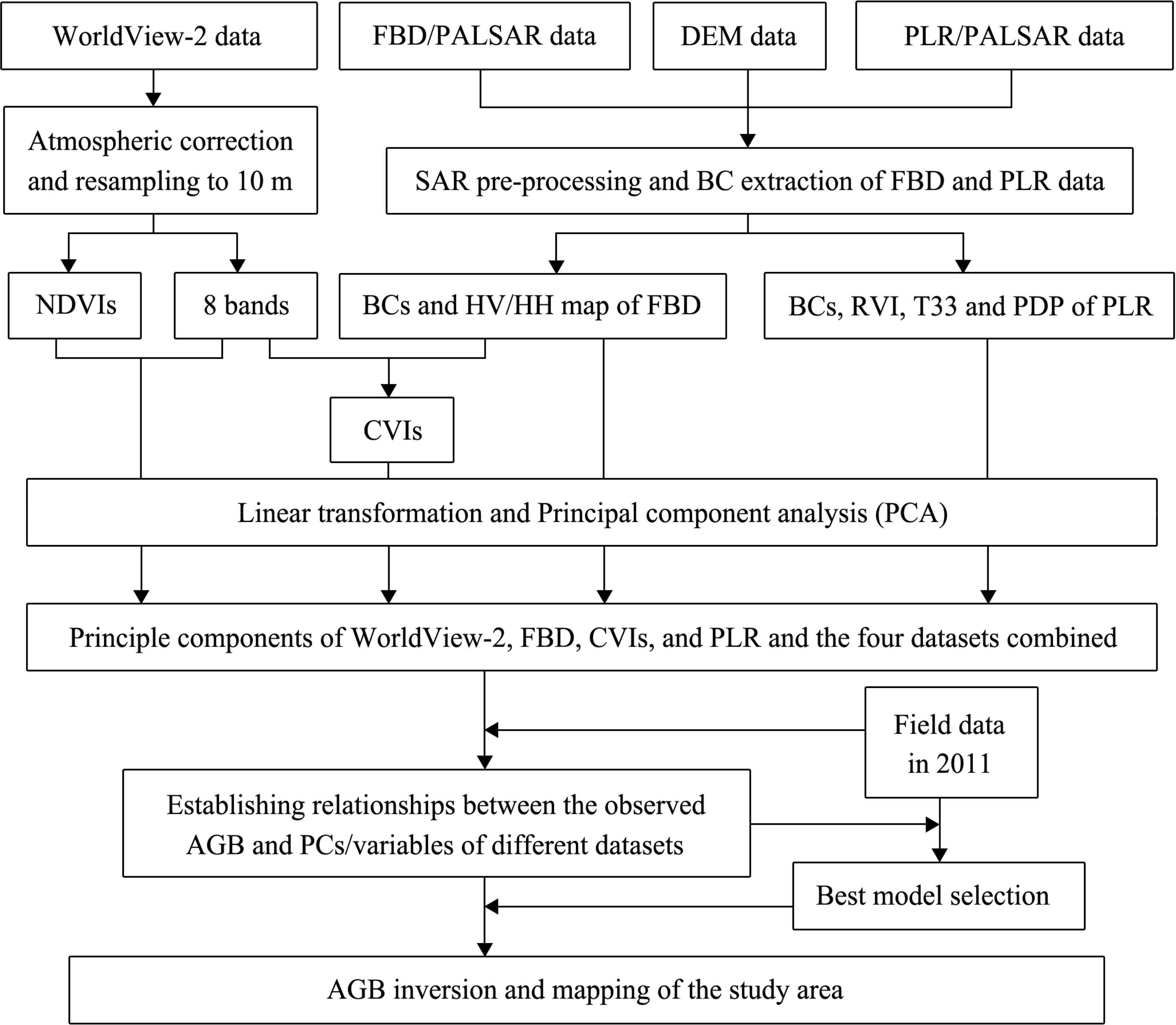
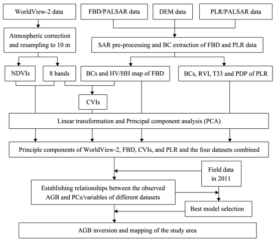
The research flow chart in Figure 2 provides an overview of the methods.
2.4.1. PALSAR Pre-Processing
The pre-processing was completed using the ENVI SARscape software. To reduce speckle and generate square pixels, the two PALSAR datasets were first multi-looked using factors of 1 and 4 for FBD image and factors of 1 and 7 for PLR data, respectively, for the range and azimuth directions. The datasets were then calibrated to obtain SAR backscattering images. The updated calibration factor provided by JAXA was used for absolute calibration [53]. In addition, the images were speckle filtered using the Lee Refined Filter during processing.
SAR data are acquired in a side-looking geometry, which leads to a number of distortions in the imagery. Terrain correction removes these geometry-induced distortions by making use of a digital elevation model (DEM). The process of terrain correction can be divided into two separate parts: geometric terrain correction and radiometric terrain correction. Geometric terrain correction adjusts the individual pixels of an amplitude image to ensure their proper location (i.e., it places the ridgelines and valleys were they geometrically belong). Radiometric terrain correction adjusts the brightness of the pixels with respect to the observation geometry, as defined by the incidence angle as well as the slope and aspect of the local terrain. Castel et al. [21] reported that areas of sloped terrain can induce 2–7 dB dispersion on radar backscattering. Therefore, the area having slopes facing the radar sensor without radiometric normalization would have higher backscatter coefficients than flatter areas, which is a problem when assessing properties of backscatter [39]. Hence, these topographic effects were addressed through radiometric normalization of the backscatter coefficient. To obtain a better representation of the backscatter coefficient for distributed targets (i.e., the forest areas), a conversion from sigma nought to gamma nought was applied [39,54]. In this study, using the DEM data with a resolution of 30 m downloaded from the ASTER GDEM website, the two images were geometrically and radiometrically terrain corrected and geo-coded to the zone 50 north of the UTM (Universal Transverse Mercator) projection and were outputted as GeoTIFF maps with a pixel size of 10 m.
2.4.2. Polarimetry and Other Parameters of the PLR/PALSAR Data
In addition to backscatter intensities, a target decomposition technique was applied to the PLR data to obtain polarimetric products. Polarimetric decomposition provides information about the scattering properties from the targets [23,55–58]. The relationships between a feature’s physical properties and its polarimetric behavior can be interpreted by examining the underlying scattering mechanisms; the scattering process can change between forest stands of different structural types and ages [39]. In our study, the entropy (H), alpha (α) angle, and anisotropy (A) decomposition parameters and the combination of H(1–A) were generated using the PolSARpro v4.2 software provided by the European Space Agency (ESA). For detailed information about these decomposition parameters, please see previous studies [23,56,58,59].
The RVI (radar vegetation index) derived from the PLR/PALSAR data can also be used to analyze the scattering from the vegetated area [60]. Woody vegetation has high cross-polarization components and high RVI values [58]. The RVI is derived from the radar backscattering coefficient (γ°) of the HH, HV, and VV polarizations [61].
In addition, the PolSARPro works with two different domains. One domain is the coherency matrix T3, which is derived from the Pauli scattering vector k. The other is the covariance matrix C3, which is based on the lexicographic scattering vector Ω. Often, the polarimetric data in the PolSARPro are stored as a T3 matrix because the diagonal matrix elements allow a physical interpretation. The T11 element represents single-bounce scattering (e.g., waters and roads), the T22 element shows the feature of double-bounce scattering (e.g., buildings), and the T33 element indicates the properties of volume scattering (e.g., forest vegetations). Therefore, the T33 map was also used to retrieve the forest AGB in our study.
2.4.3. Calculating NDVIs and CVIs (Combined Volume Index)
NDVI was selected because this vegetation index is commonly used to estimate biomass [62–65]. As shown in Figure 2, the atmospherically corrected image was used to generate the NDVI maps. To match the pixel size of the backscatter coefficient maps, the optical image had to be resampled to a spatial resolution of 10 m. Then, a standard NDVI map was produced using band 7 (NIR1) and band 5 (Red) according to the following formula:
In addition, as described in the Introduction section, optical images can provide the most information about tree crowns, such as LAI (leaf area index) and crown density, while SAR data measure forests based on backscattering from the branches and stems of the trees. Accordingly, the synergistic use of optical and SAR sensors was expected to have great potential for biomass estimation. Moreover, we determined that the observed AGB was positively correlated with the backscatter coefficient of the HV/FBD data by a moderate R2 (coefficient of determination) value and was negatively correlated with bands 1 to 6 of the WorldView-2 image fitted by a compound function expressed by the Equation (6). In our study, the trend line of this function was similar to the exponential function in the correlation with the observed biomass but had greater significance than the latter in the model test (Table 2). Therefore, a new parameter denoted the combined volume index (CVI) because of the good linear relationships between the CVIs and plot volume was generated by combining the HV backscattering of the FBD data and the eight multispectral bands of WorldView-2 image in this study. The CVI can be expressed as follows:
2.4.4. Establishing the Relationships between the Observed AGB and Parameters
In Table 2, a total of 33 variables that may be correlated with the forest biomass were first fitted with the observed AGB using the following 8 functions (Equations (5) to (12)). Then, the best-fitting equation for each variable (except for bands 7 and 8 of WorldView-2 due to their insufficient correlation with the AGB), as judged by the R2 value and significance, was used for the linear transformations. The linear-transformed variables were then used to perform the subsequent principal component analysis (PCA). Finally, the results of the PCA were used to model the biomass by multivariate stepwise regression. The coefficients (b0, b1) of the best-fitted model for each variable are listed in Table 2.
- (a)
Linear function:
- (b)
Compound function:
- (c)
Growth function:
- (d)
Logarithmic function:
- (e)
S function:
- (f)
Exponential function:
- (g)
Inverse function:
- (h)
Power function:
As shown in Table 2, most of the fitted equations are curvilinear models, indicating that implementing linear transformations for these parameters is essential before performing the multivariate linear regression (MLR). In addition, it is easily deduced that Equations (13), (14), and (15) are equivalent. Thus, the maps of these parameters fitted by curvilinear models had to be operated using the formula listed in the last column of Table 2. Moreover, because some parameters were generated from other parameters, a multicollinearity problem will remain if these parameters are directly used as independent variables to perform the multivariate stepwise regression. Consequently, on the basis of their sources, these parameters were divided into five datasets: A (FBD/ALOS), B (PLR/ALOS), C (WorldView-2), D (CVIs), and E (all 31 parameters) (Table 2). A PCA was then performed for each dataset. As a result, 2, 5, 4, 3, and 7 principal components (PC) were extracted from the dataset A to E, with cumulative variances of 99.99%, 98.31%, 99.09%, 99.56%, and 92.03%, respectively. Normality tests showed that these PCs are normally distributed. Finally, the relationships between the forest AGB and the above principal components were established using a stepwise linear regression approach.
Although MLR was the approach frequently used to predict changes in forest biomass in previous studies [41,66,67], several problems remain with these models. For example, not all variables are linearly correlated with the AGB [27,68], and thus the variables not included in the linear models should be analyzed by another statistical method. Accordingly, the artificial neural network (ANN) approach, a very useful modeling technique for non-linear problems [48], was also used to produce predictive models to estimate the AGB using the multilayer perception (MLP) algorithm. For each dataset (A, B, C, D, and E), three MLP models, called MLP1, MLP2, and MLP3, were achieved using the principal components that were included in the MLR model, using all the principal components extracted from the corresponding dataset as mentioned above, and using all the original variables (i.e., not linear-transformed) from each dataset (in datasets C and E, the bands 7 and 8 of WorldView-2 were included), respectively.
2.4.5. Error Assessments of Estimated to Observed AGB
In this study, the coefficient of determination (R2) of the actual vs. predicted AGB and the absolute and relative RMSEs (root mean square error) were used to evaluate the quality and reliability of the estimate models for forest biomass. The absolute RMSE (Mg/ha) of each biomass estimated model was calculated as SQRT(SUM(BE − BO)2/n), where BE is the estimated biomass, BO is the AGB derived from the inventory data, and n is the number of the plots. The relative RMSE (%) was defined as RMSE/Mean(BO) × 100.
3. Results
In our study, using the single variables derived from the PALSAR/ALOS and WorldView-2 data explained only approximately 20% to 50% of the variance in the plot-level measurements for the forest biomass (Table 2). Accordingly, combinations of several variables were considered to improve the relationships with the AGB.
3.1. Estimating Forest Biomass Using the FBD/PALSAR Data
Numerous studies have found that polarization ratios have advantages for biomass estimation because these ratios do not saturate as quickly as single polarization data [67,69]. Moreover, ratios are known to mitigate topographic effects [70] and to reduce forest structural effects due to forest type [71,72]. However, the relationship of the polarization ratio of the FBD data with the field biomass was worse than that of the single polarization data in our study. Thus, we attempted to investigate whether the combination of the three variables could improve the biomass estimation. Using the calibration dataset (n = 63), stepwise linear regression was first used to establish a relationship between the observed AGB as the dependent variable to be predicted and the two principal components (PC), which were extracted from the linear-transformed backscatter coefficients (HH and HV) of the FBD data and the ratio of HV to HH as possible independent variables. The regression can be expressed as the following:
Based on the multilayer perception (MLP) algorithm, the neural network approach was also used to produce several models to estimate the AGB using the FBD/PALSAR dataset (A). However, there was no MLP2 model for this dataset because the two principal components were included in the MLR model. The MLP1 and MLP3 models were created using the two PCs and directly using the values of HH, HV, and HV/HH in the FBD data, respectively. The MLP1 model for AGB estimation had a moderate fit of R2 = 0.67 with a relative RMSE of 33.48% in the validation dataset (Table 3). In other words, approximately 33% of the variance in the observed AGB was not explained by this model. The MLP3 model explained approximately 68% of the variance and showed a relative RMSE of 32.42%. There was little difference in explaining the variance between the three models derived from dataset A, possibly because the two principal components included most of the information in the dataset, with a very high cumulative variance of 99.99%.
3.2. Estimating Forest Biomass Using the PLR/PALSAR Data
Although some variables of the PLR/PALSAR data (dataset B) were significantly correlated with forest biomass, most of them had poor fits and explained less than 40% of the variance. For the purpose of increased accuracy, an MLR model was also established for the AGB estimation using the five PCs of the PLR dataset as possible independent variables. The regression can be expressed as follows:
In addition, three MLP models, called MLP1, MLP2, and MLP3, were used for the biomass estimate using the four PCs included in the MLR regression, using all five PCs extracted from the PLR/PALSAR data, and using the ten parameters that were not linear-transformed, respectively. The MLP1 and MLP2 models had the lowest fits to the observed AGB in the validation dataset, with an R2 of 0.64 and relative RMSEs of 36.38% and 36.79%, respectively. The MLP3 model explained approximately 68% of the variance and had a relative RMSE of 32.72%.
3.3. Estimating Forest Biomass Using the WorldView-2 Data
Four principal components with a cumulative variance of 99.09% were extracted from the ten linear-transformed parameters of the WorldView-2 data (except for bands 7 and 8) to perform MLR. Three of the PCs were included by the stepwise approach. The MLR model can be expressed by the following equation:
Regarding the MLP-based models, MLP1 and MLP2 were moderately correlated with the observed biomass by an R2 of 0.59 and 0.66, respectively, whereas MLP3 had the highest correlation with the AGB, which explained approximately 70% of the variance and led to a relative RMSE of 29.37%. For the WorldView-2 data, we found that the best MLP-based model (R2 = 0.70 and RMSE = 41.97 Mg/ha for the validation data) was more highly correlated with the AGB than the MLR-based model (R2 = 0.65, RMSE = 49.40 Mg/ha), primarily due to the use of bands 7 and 8 in the MLP3 model.
3.4. Estimating Forest Biomass Using the CVIs
Table 2 indicates that the eight CVI variables developed from the combination of the FBD/ALOS and WorldView-2 data had the best-fitted linear correlations with the AGB when using the eight functions (Equations (5) to (12)) to fit. Therefore, the values of the eight CVIs were directly used to perform the principal component analysis without linear transformation. Three PCs with a cumulative variance of 99.56% were extracted from the CVI dataset. Then, using the 63 calibration plots, the MLR model was obtained by the stepwise linear approach and can be expressed as the following:
In terms of the three MLP-based models, MLP1 and MLP2 only explained approximately 68% and 66% of the variance and produced a relative RMSE of 30.80% and 33.12%, respectively. The MLP3 model was the most significantly correlated to the observed AGB at the 0.001 level, with a relative RMSE of 26.51% in the validation plots (Table 3). However, in contrast to the MLR model using dataset D, a slightly poor explanation for the percentage variance was observed for the MLP3 model when validated with the independent testing dataset, possibly due to the good linear relationships between the AGB and the CVI variables.
3.5. Estimating Forest Biomass by Combining the PALSAR/ALOS and WorldView-2 Sensors
As mentioned above, modeling forest biomass using the fusion of FBD/ALOS and WorldView-2 data provided improved fits relative to their respective individual values. However, although the result is promising, no more than 80% of the variability of the field biomass could be explained by the models derived from this fusion. Previous studies have reported increased accuracy when simultaneously using several datasets from different sensors [15,30,33,48,68,73] or using SAR images from more than one date [67,74,75] or further improvement of the model. Using the 31 variables in Table 2, seven PCs with a cumulative variance of 92.03% were produced as possible independent variables to achieve the multivariate stepwise regression. According to the component matrix, the first PC was dominated by the eight CVIs, the second PC was mainly composed of the variables of the WorldView-2 dataset and called the optical factor, while the third PC was called the vegetation index factor because it was dominated by the RVI of the PLR data, the NDVIs of WorldView-2, and CVI1 to 4. The other four PCs were named as comprehensive factors. As a result, the linear model can be expressed as follows:
The MLP-based models using dataset E also showed good fits with the field biomass in our study. The MLP3 model was the most correlated to the AGB, with an R2 of 0.93 and 0.89 for the training and testing data and a relative RMSE of 13.90% and 17.06%, respectively. However, MLP1 and MLP2 explained approximately 76% and 81% of the variance and produced a relative RMSE of 26.10% and 23.48% for the validation data, respectively.
3.6. Best Estimated Model Selection and AGB Mapping in Study Area
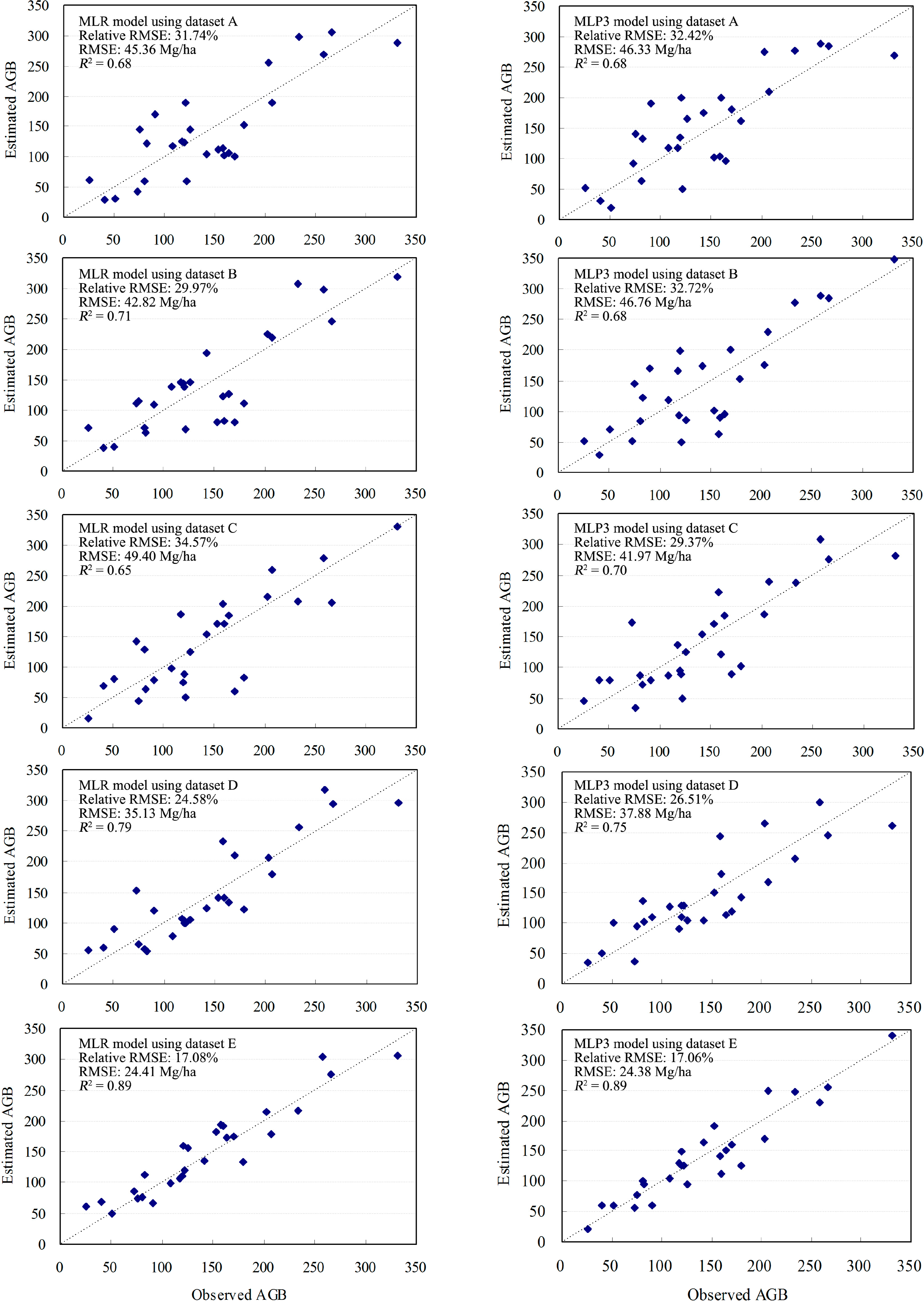
The validations of the forest biomass estimation models in Table 3 yielded the following results: (1) the MLP3 models had better fits than the MLP1 and MLP2 models, which were established using the principal components extracted from the linear-transformed variables in the five datasets, indicating the high capability of the neural network model for non-linear problems [62,68]; and (2) the validation accuracy during model development improved as the information content of the datasets increased, i.e., the best performances were obtained by the models using dataset E, followed by the models using dataset D, while using the single images produced the lowest correlations. For comparison purposes, the predicted vs. observed biomass of the testing samples (n = 27) was plotted for the MLR and MLP3 models using the five datasets and is displayed in Figure 3. The plot shows the fairly high agreements between the estimates and observations of the MLR and MLP models using dataset E.
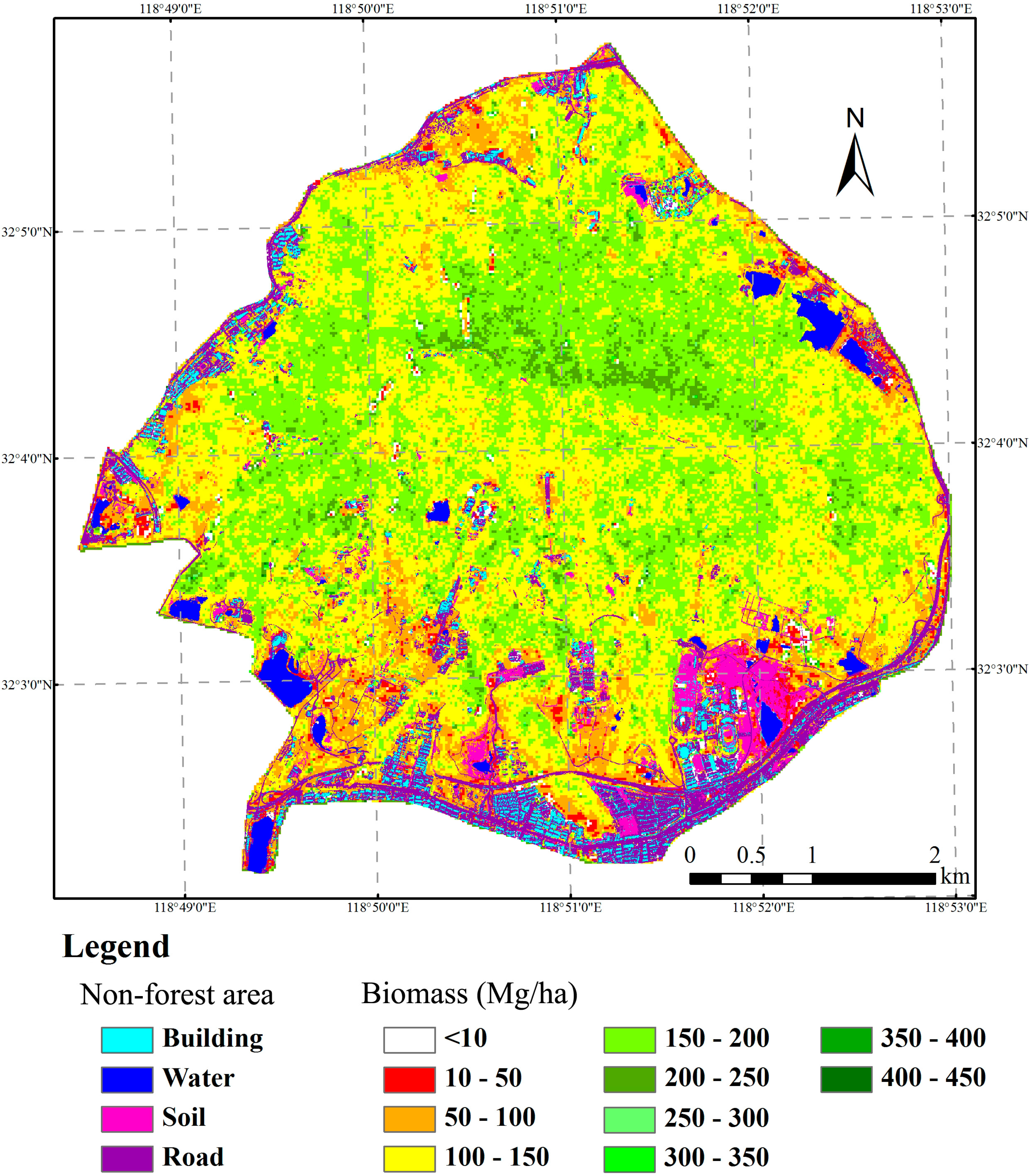
In addition, the differences in the absolute bias of the estimated vs. observed biomass between the MLR and MLP models and between the five datasets were tested by analysis of variance (ANOVA). The results suggest that the models established using dataset E exhibited a significantly lower bias at the 0.05 level than the models established using the other four datasets, while a highly consistent bias distribution was observed in the MLR and MLP3 of dataset E (F = 0.000, P = 0.995). Although the MLP3 model (R2 = 0.93) fit the AGB slightly better than the MLR model (R2 = 0.91) in the calibration plots, the two models had the same R2 = 0.89 for the testing data, indicating that the MLR model was more stable than the MLP model. In addition, the MLP-based model is more difficult to interpret than the MLR regression because it has one or more hidden layer(s) and may therefore appear to be a “black box”. Accordingly, the MLR model derived from dataset E was further used to retrieve the AGB of forests in the study area at the pixel level. The forest mask map and the land-use classification were generated in a previous study using the WorldView-2 image [44]. The overlay of the AGB map with the land-use classification is displayed in Figure 4.
The extrapolations using the predicted models for the remaining area might lead to the overestimated or underestimated biomass due to the limited number of calibration and validation plots, because these plots usually had a smaller range of AGB values than the existent in the whole study area. Consequently, the reliability of the finally recommended model was tested by the quantitative comparison of the two AGB mappings retrieved by the MLR and MLP3 models using dataset E. The two biomass maps showed a very high correlation with an R2 of 0.993. In addition, a total of 1500 random points were produced from the forest area. The AGB values of these points in the above two maps (MLR and MLP3) were then extracted for establishing a linear regression between the MLR value as the dependent variable (y) and the MLP3 value as the independent variable (x) (Figure 5). The result indicates that the two datasets were in good agreement.
3.7. The Effects of Forest Type and Vertical Structure on AGB Estimation
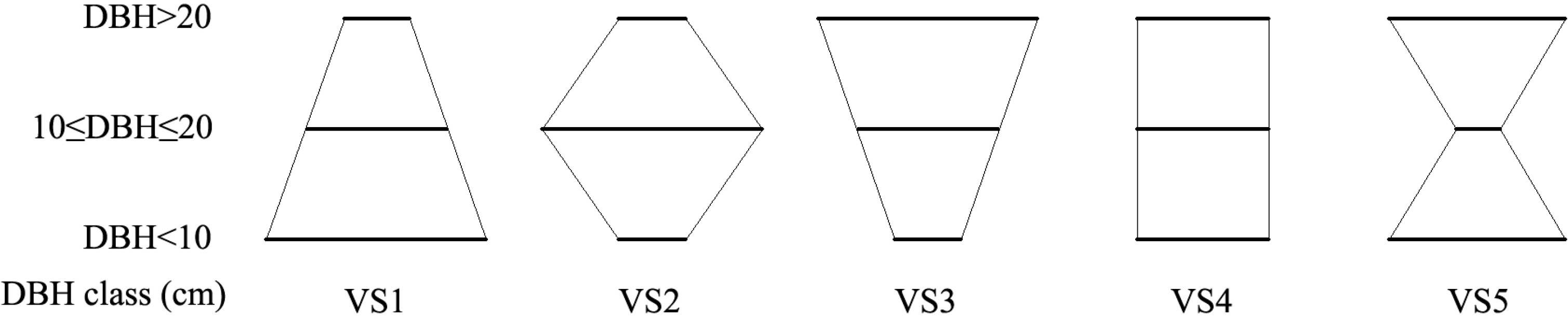
In this study, the forests in the 90 plots were divided into three types (broad-leaved, coniferous, and mixed forest, Table 1) and five vertical structures (VS1, VS2, VS3, VS4, and VS5, Figure 6) to analyze the effects of different forest types and structures on AGB retrieval. In Figure 6, the lengths of the bold lines represent the relative numbers of the stems of the three DBH classes (DBH > 20, 10 ≤ DBH ≤ 20, and DBH < 10 cm) in the plots. For example, in VS1, the ratio of stems decreased with increased DBH in a pyramid shape, while the inverse relationship was observed for VS3 in the form of an inverted pyramid. In VS5, the number of stems at 10 ≤ DBH ≤ 20 cm is far less than that at DBH > 20 and DBH < 10 cm. Due to the limited number of validation plots (n = 27), these 27 samples were divided into nine groups such that each group included a low, moderate, and high biomass plot. Then, each group with three plots was used once to replace three plots of the calibration data for achieving the MLR and MLP models using the dataset E (i.e., nine iterations), yielding a total of 270 accumulated validation samples for the accuracy assessment of the biomass estimation. The absolute and relative RMSEs of the multivariate stepwise regressions and the MLP-based models using the dataset E with 10 iterations are shown in Table 4, in which the forest types and the vertical structures are distinguished. The results indicate that the relative RMSE decreases gradually from broad-leaved to coniferous to mixed forest. VS4, in which the stem ratio was approximately the same in the 3 DBH classes, had a lower absolute RMSE, whereas VS3, in which the forest was dominated by large-size trees and lacked undergrowth trees, has the highest RMSE of the five vertical structures.
3.8. The Effects of Other Factors on AGB Estimation
Pine forests are widely distributed over a lot of countries that are counting on REDD+ programs for revenue generation through biomass conservation. With the purpose of the probable implications of our research for these countries, we analyzed the effect of the relative number of pine trees in the plots on the AGB estimates by dividing the above 270 accumulated validation samples into three groups: the relative number of pine trees ranging from 0% to 30% (PR1), 30% to 60% (PR2), and over 60% (PR3), respectively. The absolute and relative RMSEs of the three groups are documented in Table 5. The results indicate that PR2 and PR3 had lower RMSEs, whereas PR1, in which the forests were mainly dominated by broad-leaved trees, had the highest RMSEs of the three groups. In other words, the method developed by our study can be used to accurately estimate the AGB of the forests containing pine trees more than 30%.
In addition, we selected the slope and the aspect as environmental factors that could possibly impact the retrieval of the AGB. The slope was generated from the DEM with a spatial resolution of 30 m and ranged from 0° to 31° in the 90 plots. The aspect was defined as north (Azimuth ranging from 0° to 22.5° and 337.5° to 360°), northeast (22.5° to 67.5°), east (67.5° to 112.5°), southeast (112.5° to 157.5°), south (157.5° to 202.5°), southwest (202.5° to 247.5°), west (247.5° to 292.5°), and northwest (292.5° to 337.5°), and there was no flat type in the field plots. We first analyzed the relationships between the slope and the RMSEs. No significant correlations (P > 0.05) have been found, suggesting that the corrected measures mitigated the effect of different effective back-scattering surface areas caused by the local topography and SAR imagery geometry [77,78]. However, when the 270 validation samples were divided into three groups as gentle slope (GS, 0° to 10°), moderate slope (MS, 10° to 20°), and steep slope (SS, 20° to 31°) for counting estimated errors, we found that SS had the highest absolute and relative RMSEs of the three groups (Table 5). In terms of the aspects, the directions of northeast, east, southeast, south, and southwest had lower relative RMSEs less than 15%, whereas the other three directions had the relative RMSEs of approximately 20%.
4. Discussions
Mapping the spatial distribution of forest aboveground biomass is an important and challenging task. For a given ecosystem, these maps can be used to monitor forests and capture national deforestation processes; forest degradation; and the effects of conservation actions, sustainable management and the enhancement of carbon stocks [28]. In China, the national biomass estimation was mainly completed by conducting national forest inventories using the sample plotting method every five years, which is difficult to be implemented in remote areas. In recent years, although some common approaches of remote sensing have been used for estimating Chinese forest biomass on a landscape to regional scale using optical images [11,79] or SAR data [31], the development of enhanced methods (e.g., the combined use of different sensors) that can accurately retrieve forest biomass remains an important topic of study [80] due to not only the vast size of forests in China but also the limited usefulness of empirical models for different forests. Therefore, this study developed an improved approach that exploits the synergy of ALOS PALSAR and WorldView-2 data to integrate the advantages of both sensors for biomass estimation.
Although the ratio of radar backscattering is often effective for estimating forest biomass [69–72], our results did not confirm this, most likely because the SAR data were adequately geometrically and radiometrically terrain corrected to reduce topographic effects during pre-processing. Acquiring the datasets during the dry seasons (October for the FBD and March for the PLR) also helped mitigate the influence of soil and surface moisture on L-band microwave backscatter [81], which can be particularly strong when low levels of aboveground biomass are present [82]. Moreover, another reason for the poor correlation between the ratio of backscattering and the observed AGB may be the high biomass level in the study area, which is far greater than the reported saturation of approximately 60–100 Mg/ha for L-band SAR.
In our study, in addition to the backscattering coefficients of PLR/PALSAR data, several decomposition parameters, such as entropy and Alpha, and other variables (i.e., RVI and T33) were used to retrieve the AGB. Although the single variables of the PLR data had relatively low fits with the field biomass, the combined use of these variables in principal component analysis improved the estimate accuracy to approximately 71%. In addition, based on the ability of multispectral images to provide surface information about tree crowns and ability of SAR data to measure forests based on backscattering from the branches and stems of the trees, a new variable called CVI (combined volume index) was developed using the HV backscattering of the FBD data and the bands of the WorldView-2 image. The CVI dataset yielded a significant improvement in the biomass estimation compared to the use of single PALSAR or an optical sensor. Moreover, we found that the first PC extracted from the dataset E was dominated by the eight CVIs and had the highest weight in the final MLR model. Consequently, the results of this study recommend the use of these variables introduced above in the AGB estimation of forests. However, this conclusion is based on empirical models and should be further studied and verified in other forests and different seasons [41,83].
The results from this study suggest that the standard NDVI calculated from band 7 (NIR1, 0.77–0.90 μm) and band 5 (Red, 0.63–0.69 μm) of the WorldView-2 data had the lowest correlation with the surveyed AGB in the 4 NDVIs. This poor correlation reflected the saturation level reached on densely vegetated areas [41,62,64,84]. In the highly dense forests, the red band, which can be absorbed by vegetation, reaches a peak, while the reflectance of near infrared continues to increase due to multiple scattering effects [63]. Furthermore, it is likely that the WorldView-2 image was acquired in December, when the leaves of some of the tree species had fallen and the reflectance of multispectral bands was easily disturbed by the undergrowth vegetation and the ground surface, in which the forest was dominated by deciduous trees. However, we also found that many forests dominated by deciduous trees had similar reflectance characteristics with the evergreen forests by comparing their spectral features. This result probably resulted from the distribution of evergreen broad-leaved trees under the deciduous trees. Accordingly, the difference of the reflectance between deciduous and evergreen broad-leaved forests in the study area needs to be clarified by further study using another WorldView-2 image acquired in summer.
In addition, we found that the developed NDVIs computed from the NIRs and the additional red-edge band were slightly better fitted to the AGB than those calculated from the NIRs and the red band. This result was consistent with previous studies indicating that red-edge or longer wavelengths result in higher correlations with biomass in dense vegetations than the standard NDVI [13]. The indices calculated from the red-edge may be more sensitive to vegetation properties such as canopy biomass and chlorophyll content than other electromagnetic spectrums [9,85]. A slight change in these vegetation properties will lead to a shift in the red-edge curve [86]. In addition, the expanded NDVIs computed from the red-edge and NIRs can mitigate the effects of the atmospheric and water absorption and soil background [87]. As a consequence, the additional bands of the WorldView-2 satellite are able to estimate biomass in highly dense forests. However, these bands should be further tested by application to other forests during different seasons.
Most previous studies used a simple logarithmic or exponential function to establish relationships between the AGB and the backscattering coefficients of the SAR data [19,28,31,88]. However, when using the eight functions listed in the methods section for fitting, we determined that the variables had different best-fitted models, as judged by the R2 value and significance. For most parameters of PALSAR data, the compound and growth functions had better fits than the other functions. In fact, the trend lines of the two functions were similar to those of the exponential or logarithmic functions in correlation with the observed biomass, but they had higher significance than the latter in the model test. Finding the best-fitted function is favorable for the improvement of AGB retrieval when using the MLR method to estimate the biomass because implementing linear transformations for these curvilinear-correlated variables is essential before performing the multivariate stepwise regression. However, the neural network approach did not improve the AGB estimation when using linear transformations, as indicated by the higher correlation with the observed biomass for the MLP3 models than for the MLP1 and MLP2 models in the five datasets.
MLR is a common approach used for estimating the biomass of forests [41,66,67]. However, with the increasingly synergistic use of different sensors, the MLR method has some limitations, e.g., the estimate accuracy no longer improves when additional variables are added [30] because not all parameters are linearly correlated with the biomass [14,27,62,65]. Accordingly, for the purpose of comparison with the multivariate stepwise regression, the neural network approach was also used to develop several estimated models using the multilayer perception algorithm. Several studies have indicated that the neural network approach significantly improves forest biomass estimation [10,27,48,62,68]. However, in this study, the results obtained using the network approach were inconsistent for different datasets. Overall, the MLP3 models had slightly better fits to the field biomass in the calibration plots. However, for dataset D, the MLP models were more poorly fitted to the AGB than the MLR model in the training and testing plots. The superior fit of the MLR model may be due to the good linear correlations between the biomass and the CVI variables. In terms of dataset E, although the MLP3 model was slightly better correlated with the AGB than the MLR model in the calibration plots, the two models had the same R2 value for the testing data, suggesting that the MLR model was more stable than the MLP model. As a result, our study recommended using the final MLR model rather than the MLP approach to map the AGB in the study area.
Figure 4 suggests that the final stepwise model can be used to retrieve the forest biomass when the AGB level is approximately 10 Mg/ha to 450 Mg/ha, levels that are typical of most subtropical and warm temperate zone forests in China [52], indicating that the approach generated by our study can provide some knowledge for AGB estimation in China. However, slightly lower R2 values and higher RMSEs were obtained in our study compared with previous studies [31,39,47,67,75]. Several factors may explain the relatively poor results. First, to contain the biomass levels of the study area, we investigated plots with AGBs that ranged from approximately 25 to 342 Mg/ha. Because no AGB plots lower than 60 Mg/ha were found in the closed stand, some plots with lower biomasses had to be located in open forest land, where the reflectance of remote sensors is easily affected by the ground surface, leading to high RMSEs at these plots. For example, the reflectance of NIRs in the closed forest is evidently higher than that in open forest land. Second, the inexact calculation of the observed AGB could also lead to a high RMSE. Generally, the biomass of individual trees in the plot can be accurately estimated using allometric equations on the basis of the DBH and the height of the trees [16,31,51]. However, no allometric equations were available for the study area, indicating that further basic research is needed in this region. Therefore, we had to use the method presented by [52], in which the biomass of each plot is estimated from the regression of the biomass and the total volume of the plot. Although this method is considered accurate for AGB estimation over a large area and has been adopted by numerous researchers, the accuracy must be improved by incorporating more forest field data on a regional scale.
Moreover, we have analyzed the effects of different forest types and vertical structures on the biomass estimate. In terms of forest types, the RMSE decreases gradually from broad-leaved to coniferous to mixed forest. In the study area, most of the broad-leaved stands are composed of secondary forests derived from clear-cutting of the land. These stands have disorganized structures and lower AGBs, resulting in a higher RMSE for broad-leaved forest than for the other stands. However, the coniferous forests, which have a regular spatial structure and a higher AGB, are derived from manmade plantations that were planted approximately 60 to 80 years ago. The mixed forests are mainly composed of coniferous trees with large sizes distributed in the upper layer and broad-leaved trees in the understory. These forests have a complicated spatial structure and high canopy density, increasing their sensitivity to the signals of both SAR and optical sensors and reducing ground surface effects. Of the five vertical structures, VS3 has the highest errors because the forest lacks undergrowth trees; the absence of undergrowth trees reduces the random scattering of the forest and enhances the single reflection of the ground surface on the SAR. By contrast, the VS4 forest, which has approximately same ratio of stems as the three DBH classes, has a complex spatial structure in which the scattering is characterized by a high degree of randomness and thus has the lowest estimated error.
Finally, we have analyzed the effects of the relative numbers of pine trees in plots, slopes, and aspects on the AGB estimation. We found that the PR1 group, in which the relative number of pine trees in the plots ranged from 0% to 30%, has higher average RMSEs than the other two groups, because most plots in PR1 were dominated by broad-leaved forests. By contrast, PR2 has the lowest RMSEs of the three groups, because most plots in PR2 were composed of mixed forests that had lower estimated errors than other forest types. Additionally, although no significant correlations between the slope and the RMSEs have been found, the plots within steep slope had the highest average error. Two reasons may explain this result. First, the DEM data with a spatial resolution of 30 m was used for geometric and radiometric terrain correction, which is difficult to mitigate the effect of the steep topography on the back-scattering [21,78]. Consequently, this issue requests future studies using a high resolution DEM. Second, many forests in the plots within steep slope had the vertical structure of VS3 that had the highest estimated error of the five vertical structures. In terms of aspects, the plots facing the directions of west, northwest, and north had higher estimated errors than those facing other directions. The steep topography of the three directions, which had an average slope of 14°, 13°, and 11°, respectively, probably leads to this result.
5. Conclusions
In our study, the single variables derived from the PALSAR/ALOS and WorldView-2 data correlated very poorly with the observed biomass and were able to explain only approximately 20% to 50% of the variance. Accordingly, combinations of several variables were considered to improve the relationship with the AGB. Using principal component analysis and multivariate stepwise regression, the performances of the FBD, PLR, and optical data for biomass estimation were improved to 65% to 71%. In addition, using the additional dataset derived from the combination of FBD/PALSAR and WorldView-2 data increased the performance to 79% and produced a relative RMSE of 24.58% when using MLR. Moreover, the synergistic use of the 31 variables introduced by our study resulted in further improvement, ultimately explaining 89% of the variance with a relative RMSE of 17.08%. The results presented here demonstrate that combining independent observation data from the PALSAR and WorldView-2 sources may provide great improvements for biomass estimation in the study area. However, because most biomass models or regressions are developed for specific locations, the models generated by our study should be further tested by application to other forests during different seasons. In addition, for the purpose of comparison with the multivariate stepwise regression, a neural network approach using the multilayer perception (MLP) algorithm was used to produce several estimated models of forest biomass. However, few improvements were obtained from the MLP approach in this study. Consequently, we recommend using the final MLR model to map the AGB of the study area. Finally, analyzing the effects of different forest types and vertical structures on the biomass estimation revealed that the RMSE decreased gradually from broad-leaved to coniferous to mixed forest. In terms of different vertical structures, VS3 had the highest errors because the forest lacks undergrowth trees, while the VS4 forest, in which the three DBH classes have approximately the same ratio of stems, had the lowest RMSE.
Acknowledgments
This study was supported by a Grant-in-Aid for Scientific Research from the Japan Society for the Promotion of Science (No. 24380077), the National Basic Research Program of China (973 program, 2012CB416904), and the Natural Science Foundation of China (Grant No. 50978054, MCDA/GIS-based spatial decision making method for recreational forest in open urban space). We gratefully acknowledge a number of students of Nanjing Forestry University for their support in the field and the plot survey. We would like to thank the members of the Forest Ecology Laboratory, Nanjing Forestry University, for their advice and assistance with this study. Moreover, we acknowledge the helpful comments of the three anonymous reviewers and editor.
Author Contributions
Songqiu Deng designed the experiment. Masato Katoh, Qingwei Guan and Mingyang Li coordinated the research projects and gave technical supports and conceptual advice. Songqiu Deng, Qingwei Guan and Na Yin performed the experiment and collected the data. Mingyang Li provided the basic data and calculated the aboveground biomass. Songqiu Deng and Na Yin analyzed the data and wrote the paper. Qingwei Guan and Mingyang Li served as scientific advisors. Songqiu Deng, Masato Katoh, Qingwei Guan, Na Yin and Mingyang Li helped in preparation and revision of the manuscript.
Conflicts of Interest
The authors declare no conflict of interest.
References
- Canadell, J.; Ciais, P.; Cox, P.; Heimann, M. Quantifying, understanding and managing the carbon cycle in the next decades. Climatic Change 2004, 67, 147–160. [Google Scholar]
- Campbell, B. Beyond Copenhagen: REDD plus, agriculture, adaptation strategies and poverty. Glob. Environ. Change-Human and Policy Dimens 2009, 19, 397–399. [Google Scholar]
- Peregon, A.; Yamagata, Y. The use of ALOS/PALSAR backscatter to estimate above-ground forest biomass: A case study in Western Siberia. Remote Sens. Environ 2013, 137, 139–146. [Google Scholar]
- Gibbs, H.K.; Brown, S.; Niles, J.O.; Foley, J.A. Monitoring and estimating tropical forest carbon stocks: Making REDD a reality. Environ. Res. Lett 2007, 2. [Google Scholar] [CrossRef]
- Herold, M.; Johns, T. Linking requirements with capabilities for deforestation monitoring in the context of the UNFCCC-REDD process. Environ. Res. Lett 2007, 2. [Google Scholar] [CrossRef]
- Avitabile, V.; Baccini, A.; Friedl, M.A.; Schmullius, C. Capabilities and limitations of Landsat and land cover data for aboveground woody biomass estimation of Uganda. Remote Sens. Environ 2012, 117, 366–380. [Google Scholar]
- Franklin, J. Thematic mapper analysis of coniferous forest structure and composition. Int. J. Remote Sens 1986, 7, 1287–1301. [Google Scholar]
- Steininger, M. Satellite estimation of tropical secondary forest above-ground biomass: Data from Brazil and Bolivia. Int. J. Remote Sens 2000, 21, 1139–1157. [Google Scholar]
- Ozdemir, I.; Karnieli, A. Predicting forest structural parameters using the image texture derived from WorldView-2 multispectral imagery in a dryland forest, Israel. Int. J. Appl. Earth Obs. Geoinf 2011, 13, 701–710. [Google Scholar]
- Foody, G.M.; Boyd, D.S.; Cutler, M.E.J. Predictive relations of tropical forest biomass from Landsat TM data and their transferability. Remote Sens. Environ 2003, 85, 463–474. [Google Scholar]
- Zheng, G.; Chen, J.M.; Tian, Q.J.; Ju, W.M.; Xia, X.Q. Combining remote sensing imagery and forest age inventory for biomass mapping. J. Environ. Manag 2007, 85, 616–623. [Google Scholar]
- Powell, S.L.; Cohen, W.B.; Healey, S.P.; Kennedy, R.E.; Moisen, G.G.; Pierce, K.B.; Ohmann, J.L. Quantification of live aboveground forest biomass dynamics with Landsat time-series and field inventory data: A comparison of empirical modeling approaches. Remote Sens. Environ 2010, 114, 1053–1068. [Google Scholar]
- Mutanga, O.; Skidmore, A.K. Narrow band vegetation indices overcome the saturation problem in biomass estimation. Int. J. Remote Sens 2004, 25, 3999–4014. [Google Scholar]
- Labrecque, S.; Fournier, R.A.; Luther, J.E.; Piercey, D. A comparison of four methods to map biomass from Landsat-TM and inventory data in western Newfoundland. For. Ecol. Manag 2006, 226, 129–144. [Google Scholar]
- Duncanson, L.; Niemann, K.; Wulder, M. Integration of GLAS and Landsat TM data for aboveground biomass estimation. Can. J. Remote Sens 2010, 36, 129–141. [Google Scholar]
- Lu, D.S. The potential and challenge of remote sensing-based biomass estimation. Int. J. Remote Sens 2006, 27, 1297–1328. [Google Scholar]
- Wulder, M.A. Optical remote-sensing techniques for the assessment of forest inventory and biophysical parameters. Prog. Phys. Geogr 1998, 22, 449–476. [Google Scholar]
- Wang, Y.; Kasischke, E.S.; Melack, J.M.; Davis, F.W.; Christensen, N.L., Jr. The effects of changes in loblolly pine biomass and soil moisture on ERS-1 SAR backscatter. Remote Sens. Environ 1994, 49, 25–31. [Google Scholar]
- Hamdan, O.; Aziz, H.K.; Rahman, K.A. Remotely sensed L-Band SAR data for tropical forest biomass estimation. J. Trop. For. Sci 2011, 23, 318–327. [Google Scholar]
- Dobson, M.C.; Ulaby, F.T.; LeToan, T.; Beaudoin, A.; Kasischke, E.S.; Christensen, N. Dependence of radar backscatter on coniferous forest biomass. IEEE Trans. Geosci. Remote Sens 1992, 30, 412–415. [Google Scholar]
- Castel, T.; Beaudoin, A.; Stach, N.; Stussi, N.; Le Toan, T.; Durand, P. Sensitivity of space-borne SAR data to forest parameters over sloping terrain. Theory and experiment. Int. J. Remote Sens 2001, 22, 2351–2376. [Google Scholar]
- Sandberg, G.; Ulander, L.M.H.; Fransson, J.E.S.; Holmgren, J.; Le Toan, T. L and P-band backscatter intensity for biomass retrieval in hemiboreal forest. Remote Sens. Environ 2011, 115, 2874–2886. [Google Scholar]
- Cloude, S.R.; Pottier, E. An entropy based classification scheme for land applications of polarimetric SAR. IEEE Trans. Geosci. Remote Sens 1997, 35, 68–78. [Google Scholar]
- Englhart, S.; Keuck, V.; Siegert, F. Aboveground biomass retrieval in tropical forests—The potential of combined X- and L-band SAR data use. Remote Sens. Environ 2011, 115, 1260–1271. [Google Scholar]
- Rosenqvist, A.; Shimada, M.; Ito, N.; Watanabe, M. ALOS PALSAR: A pathfinder mission for global-scale monitoring of the environment. IEEE Trans. Geosci. Remote Sens 2007, 45, 3307–3316. [Google Scholar]
- Hoan, N.T.; Tateishi, R.; Alsaaideh, B.; Ngigi, T.; Alimuddin, I.; Johnson, B. Tropical forest mapping using a combination of optical and microwave data of ALOS. Int. J. Remote Sens 2013, 34, 139–153. [Google Scholar]
- Santos, J.R.; Freitas, C.C.; Araujo, L.S.; Dutra, L.V.; Mura, J.C.; Gama, F.F.; Soler, L.S.; Sant’Anna, S.J.S. Airborne P-band SAR applied to the aboveground biomass studies in the Brazilian tropical rainforest. Remote Sens. Environ 2003, 87, 482–493. [Google Scholar]
- Carreiras, J.M.B.; Vasconcelos, M.J.; Lucas, R.M. Understanding the relationship between aboveground biomass and ALOS PALSAR data in the forests of Guinea-Bissau (West Africa). Remote Sens. Environ 2012, 121, 426–442. [Google Scholar]
- Cartus, O.; Santoro, M.; Kellndorfer, J. Mapping forest aboveground biomass in the Northeastern United States with ALOS PALSAR dual-polarization L-band. Remote Sens. Environ 2012, 124, 466–478. [Google Scholar]
- Häme, T.; Rauste, Y.; Antropov, O.; Ahola, H.A.; Kilpi, J. Improved mapping of tropical forests with optical and SAR imagery, Part II: Above ground biomass estimation. IEEE J. Sel. Top. Appl. Earth Obs. Remote Sens 2013, 6, 92–101. [Google Scholar]
- He, Q.S.; Cao, C.X.; Chen, E.X.; Sun, G.Q.; Ling, F.L.; Pang, Y.; Zhang, H.; Ni, W.J.; Xu, M.; Li, Z.Y.; et al. Forest stand biomass estimation using ALOS PALSAR data based on LiDAR-derived prior knowledge in the Qilian Mountain, western China. Int. J. Remote Sens 2012, 33, 710–729. [Google Scholar]
- Lefsky, M.A.; Cohen, W.B.; Acker, S.A.; Parker, G.G.; Spies, T.A.; Harding, D. Lidar remote sensing of the canopy structure and biophysical properties of Douglas-fir western hemlock forests. Remote Sens. Environ 1999, 70, 339–361. [Google Scholar]
- Montesano, P.M.; Cook, B.D.; Sun, G.; Simard, M.; Nelson, R.F.; Ranson, K.J.; Zhang, Z.; Luthcke, S. Achieving accuracy requirements for forest biomass mapping: A spaceborne data fusion method for estimating forest biomass and LiDAR sampling error. Remote Sens. Environ 2013, 130, 153–170. [Google Scholar]
- Popescu, S.C.; Wynne, R.H.; Scrivani, J.A. Fusion of small-footprint LiDAR and multi-spectral data to estimate plot-level volume and biomass in deciduous and pine forests in Virginia, USA. For. Sci 2004, 50, 551–565. [Google Scholar]
- Næsset, E.; Gobakken, T. Estimation of above- and below-ground biomass across regions of the boreal forest zone using airborne laser. Remote Sens. Environ 2008, 112, 3079–3090. [Google Scholar]
- Zhao, K.G.; Popescu, S.; Nelson, R. LiDAR remote sensing of forest biomass: A scale in variant estimation approach using airborne lasers. Remote Sens. Environ 2009, 113, 182–196. [Google Scholar]
- Boudreau, J.; Nelson, R.; Margolis, H.; Beaudoin, A.; Guindon, L.; Kimes, D. Regional aboveground forest biomass using airborne and spaceborne LiDAR in Québec. Remote Sens. Environ 2008, 112, 3876–3890. [Google Scholar]
- Mitchard, E.T.A.; Saatchi, S.S.; White, L.J.T.; Abernethy, K.A.; Jeffery, K.J.; Lewis, S.L.; Collins, M.; Lefsky, M.A.; Leal, M.E.; Woodhouse, I.H.; et al. Mapping tropical forest biomass with radar and spaceborne LiDAR in Lopé National Park, Gabon: Overcoming problems of high biomass and persistent cloud. Biogeosciences 2012, 9, 179–191. [Google Scholar]
- Tsui, O.W.; Coops, N.C.; Wulder, M.A.; Marshall, P.L.; McCardle, A. Using multi-frequency radar and discrete-return LiDAR measurements to estimate above-ground biomass and biomass components in a coastal temperate forest. ISPRS J. Photogram. Remote Sens 2012, 69, 121–133. [Google Scholar]
- Nelson, R.; Kimes, D.S.; Salas, W.A.; Routhier, M. Secondary forest age and tropical forest biomass estimation using thematic mapper imagery. BioScience 2000, 50, 419–431. [Google Scholar]
- Zheng, D.; Rademacher, J.; Chen, J.; Crow, T.; Bresee, M.; Moine, J.L.; Ryu, S.R. Estimating aboveground biomass using Landsat 7 ETM+ data across a managed landscape in northern Wisconsin, USA. Remote Sens. Environ 2004, 93, 402–411. [Google Scholar]
- Omar, H. Commercial timber tree species identification using multispectral worldview-2 data. In 8-Bands Research Challenge; Digital Globe: Longmont, CO, USA, 2010. [Google Scholar]
- Immitzer, M.; Atzberger, C.; Koukal, T. Tree species classification with random forest using very high spatial resolution 8-band WorldView-2 satellite data. Remote Sens 2012, 4, 2661–2693. [Google Scholar]
- Deng, S.; Katoh, M.; Guan, Q.; Yin, N.; Li, M. Interpretation of forest resources at the individual tree level at Purple Mountain, Nanjing City, China, using WorldView-2 imagery by combining GPS, RS and GIS technologies. Remote Sens 2014, 6, 87–110. [Google Scholar]
- Peerbhay, K.Y.; Mutanga, O.; Ismail, R. Investigating the capability of few strategically placed Worldview-2 multispectral bands to discriminate forest species in KwaZulu-Natal, South Africa. IEEE J. Sel. Top. Appl. Earth Obs. Remote Sens 2014, 7, 307–316. [Google Scholar]
- Eckert, S. Improved forest biomass and carbon estimations using texture measures from WorldView-2 satellite data. Remote Sens 2012, 4, 810–829. [Google Scholar]
- Sun, G.; Ranson, K.J.; Guo, Z.; Zhang, Z.; Montesano, P.; Kimes, D. Forest biomass mapping from Lidar and radar synergies. Remote Sens. Environ 2011, 115, 2906–2916. [Google Scholar]
- Cutler, M.E.J.; Boyd, D.S.; Foody, G.M.; Vetrivel, A. Estimating tropical forest biomass with a combination of SAR image texture and Landsat TM data: An assessment of predictions between regions. ISPRS J. Photogram. Remote Sens 2012, 70, 66–77. [Google Scholar]
- State Forestry Administration of China. The Main Results of the 7th National Forest Resource Inventory (2004–2008). 2010. Available online: http://www.forestry.gov.cn/portal/main/s/65/content-326341.html (accessed on 10 December 2013). (In Chinese). [Google Scholar]
- Jiangsu Forestry Investigation and Planning Institute. Report on the Forest Resources of the Purple Mountain National Park; Purple Mountain National Park Administration: Nanjing, China, 2002; pp. 1–183. (In Chinese) [Google Scholar]
- Chave, J.; Andalo, C.; Brown, S.; Cairns, M.A.; Chambers, J.Q.; Eamus, D.; Folster, H.; Fromard, F.; Higuchi, N.; Kira, T.; et al. Tree allometry and improved estimation of carbon stocks and balance in tropical forests. Oecologia 2005, 145, 87–99. [Google Scholar]
- Fang, J.; Liu, G.; Xu, S. Biomass and net production of forest vegetation in China. Acta. Ecol. Sin 1996, 16, 497–508, (In Chinese with English abstract). [Google Scholar]
- Shimada, M.; Isoguchi, O.; Tadono, I.; Isono, K. PALSAR polarimetric calibration and geometric calibration. IEEE Trans. Geosci. Remote Sens 2009, 47, 3915–3932. [Google Scholar]
- Kim, C. Quantataive analysis of relationship between ALOS PALSAR backscatter and forest stand volume. J. Marine Sci. Tech 2012, 20, 624–628. [Google Scholar]
- Freeman, A.; Durden, S.L. A three-component scattering model for Polarimetric SAR data. IEEE Trans. Geosci. Remote Sens 1998, 36, 963–973. [Google Scholar]
- Yamaguchi, Y.; Moriyama, T.; Ishido, M.; Yamada, H. Four-component scattering model for Polarimetric SAR image decomposition. IEEE Trans. Geosci. Remote Sens 2005, 43, 1699–1706. [Google Scholar]
- Van Zyl, J.J.; Arii, M.; Kim, Y. Model-Based decomposition of Polarimetric SAR covariance matrices constrained for nonnegative eigenvalues. IEEE Trans. Geosci. Remote Sens 2011, 49, 3452–3459. [Google Scholar]
- Avtar, R.; Sawada, H.; Takeuchi, W.; Singh, G. Characterization of forests and deforestation in Cambodia using ALOS/PALSAR observation. Geocarto. Int 2012, 27, 119–137. [Google Scholar]
- Cloude, S.R.; Pottier, E. A review of target decomposition theorems in radar Polarimetry. IEEE Trans. Geosci. Remote Sens 1996, 34, 498–518. [Google Scholar]
- Qi, Z.; Yeh, A.G.; Li, X.; Lin, Z. Land use and land cover classification using RADARSAT-2 polarimetric SAR image. Int. Arch. Photogram. Remote Sens 2010, XXXVIII, 198–203. [Google Scholar]
- Kim, Y.; van Zyl, J. Comparison of forest parameter estimation techniques using SAR data. In Proceedings of IEEE 2001 International Geoscience and Remote Sensing Symposium (IGARSS), Sydney, NSW, Australia, 9–13 July 2001; pp. 1395–1397.
- Foody, G.M.; Cutler, M.E.; McMorrow, J.; Pelz, D.; Tangki, H.; Boyd, D.S.; Douglas, I. Mapping the biomass of Bornean tropical rain forest from remotely sensed data. Glob. Ecol. Biogeogr 2001, 10, 379–387. [Google Scholar]
- Dong, J.; Kaufmann, R.K.; Myneni, R.B.; Tucker, C.J.; Kauppi, P.E.; Liski, J.; Buermann, W.; Alexeyev, V.; Hughes, M.K. Remote sensing estimates of boreal and temperate forest woody biomass: carbon pools, sources, and sinks. Remote Sens. Environ 2003, 84, 393–410. [Google Scholar]
- Tan, K.; Piao, S.; Peng, C.; Fang, J. Satellite-based estimation of biomass carbon stocks for northeast China’s forests between 1982 and 1999. For. Ecol. Manag 2007, 240, 114–121. [Google Scholar]
- Soenen, S.A.; Peddle, D.R.; Hall, R.J.; Coburn, C.A.; Hall, F.G. Estimating aboveground forest biomass from canopy reflectance model inversion in mountainous terrain. Remote Sens. Environ 2010, 114, 1325–1337. [Google Scholar]
- Kasischke, E.S.; Christensen, N.L.; Bourgeau-Chavez, L.L. Correlating radar backscatter with components of biomass in loblolly pine forests. IEEE Trans. Geosci. Remote Sens 1995, 33, 643–659. [Google Scholar]
- Sarker, M.L.R.; Nichol, J.; Ahmad, B.; Busu, I.; Rahman, A.A. Potential of texture measurements of two-date dual polarization PALSAR data for the improvement of forest biomass estimation. ISPRS J. Photogram. Remote Sens 2012, 69, 146–166. [Google Scholar]
- Amini, J.; Tetuko Sri Sumantyo, J. Employing a method on SAR and optical images for forest biomass estimation. IEEE Trans. Geosci. Remote Sens 2009, 47, 4020–4026. [Google Scholar]
- Harrell, P.A.; Kasischke, E.S.; Bourgeau-Chavez, L.L.; Haney, E.M.; Christensen, N.L., Jr. Evaluation of approaches aboveground biomass in using SIR-C data. Remote Sens. Environ 1997, 59, 223–233. [Google Scholar]
- Ranson, K.J.; Sun, G.; Kharuk, V.I.; Kovacs, K. Characterization of forests in Western Sayani Mountains, Siberia from SAR data. Remote Sens. Environ 2001, 75, 188–200. [Google Scholar]
- Dobson, M.C.; Ulaby, F.T.; Pierce, L.E.; Sharik, T.L.; Bergen, K.M.; Kellndorfer, J.; Kendra, J.R.; Li, E.; Lin, Y.C.; Nashashibi, A.; et al. Estimation of forest biomass characteristics in northern Michigan with SIR-C/XSAR data. IEEE Trans. Geosci. Remote Sens 1995, 33, 877–894. [Google Scholar]
- Foody, G.M.; Green, R.M.; Curran, P.J.; Lucas, R.M.; Honzak, M.; Do Amaral, I. Observations on the relationship between SIR-C radar backscatter and the biomass of regenerating tropical forests. Int. J. Remote Sens 1997, 18, 687–694. [Google Scholar]
- Cohen, W.B.; Spies, T.A. Estimating structural attributes of Douglas-fir/western hemlock forest stands from Landsat and Spot imagery. Remote Sens. Environ 1992, 41, 1–17. [Google Scholar]
- Kurvonen, L.; Pulliainen, J.; Hallikainen, M. Retrieval of biomass in boreal forests from multi-temporal ERS-1 and JERS-1 SAR data. IEEE Trans. Geosci. Remote Sens 1999, 37, 198–205. [Google Scholar]
- Englhart, S.; Keuck, V.; Siegert, F. Modeling aboveground biomass in tropical forests using Multi-Frequency SAR data—A comparison of methods. IEEE J. Sel. Top. Appl. Earth Obs. Remote Sens 2012, 5, 298–306. [Google Scholar]
- Ghasemi, N.; Sahebi, M.R.; Mohammadzadeh, A. Biomass estimation of a temperate deciduous forest using wavelet analysis. IEEE Trans. Geosci. Remote Sens 2012, 51, 765–776. [Google Scholar]
- Ulander, L.M.H. Radiometric slope correction of synthetic-aperture radar images. IEEE Trans. Geosci. Remote Sens 1996, 34, 1115–1122. [Google Scholar]
- Shimada, M.; Hirosawa, H. Slope corrections to normalized RCS using SAR interferometry. IEEE Trans. Geosci. Remote Sens 2000, 38, 1479–1484. [Google Scholar]
- Gao, Y.; Liu, X.; Min, C.; He, H.; Yu, G.; Liu, M.; Zhu, X.; Wang, Q. Estimation of the North–South transect of Eastern China forest biomass using remote sensing and forest inventory data. Int. J. Remote Sens 2013, 34, 5598–5610. [Google Scholar]
- Tian, X.; Su, Z.; Chen, E.; Li, Z.; van der Tol, C.; Guo, J.; He, Q. Estimation of forest above-ground biomass using multi-parameter remote sensing data over a cold and arid area. Int. J. Appl. Earth Obs. Geoinf 2012, 14, 160–168. [Google Scholar]
- Lucas, R.; Armston, J.; Fairfax, R.; Fensham, R.; Accad, A.; Carreiras, J.; Kelley, J.; Bunting, P.; Clewley, D.; Bray, S.; et al. An evaluation of the ALOS PALSAR L-band backscatter-above ground biomass relationship Queensland, Australia: Impacts of surface moisture condition and vegetation structure. IEEE J. Sel. Top. Appl. Earth Obs. Remote Sens 2010, 3, 576–593. [Google Scholar]
- Kasischke, E.S.; Tanase, M.A.; Bourgeau-Chavez, L.L.; Borr, M. Soil moisture limitations on monitoring boreal forest regrowth using spaceborne L-band SAR data. Remote Sens. Environ 2011, 115, 227–232. [Google Scholar]
- Gobron, N.; Pinty, B.; Verstraete, M.M. Theoretical limits to the estimation of the leaf area index on the basis of visible and near-infrared remote sensing data. IEEE Trans. Geosci. Remote Sens 1997, 35, 1438–1445. [Google Scholar]
- Nichol, J.E.; Sarker, M.L.R. Improved biomass estimation using the texture parameters of two high-resolution optical sensors. IEEE Trans. Geosci. Remote Sens 2011, 49, 930–948. [Google Scholar]
- Filella, I.; Penuelas, J. The red edge position and shape as indicators of plant chlorophyll content, biomass and hydric status. Int. J. Remote Sens 1994, 15, 1459–1470. [Google Scholar]
- Lucas, N.S.; Curran, P.J.; Plummer, S.E.; Danson, F.M. Estimating the stem carbon production of a coniferous forest using an ecosystem simulation model driven by the remotely sensed red edge. Int. J. Remote Sens 2000, 21, 619–631. [Google Scholar]
- Kokaly, R.F.; Clark, R.N. Spectroscopic determination of leaf biochemistry using band-depth analysis of absorption features and stepwise multiple linear regression. Remote Sens. Environ 1999, 67, 267–287. [Google Scholar]
- Morel, A.C.; Saatchi, S.S.; Malhi, Y.; Berry, N.J.; Banin, L.; Burslem, D.; Nilus, R.; Ong, R.C. Estimating aboveground biomass in forest and oil palm plantation in Sabah, Malaysian Borneo using ALOS PALSAR data. For. Ecol. Manag 2011, 262, 1786–1798. [Google Scholar]


| No. | Density (Stem/ha) | Average DBH (cm) | Average Height (m) | AGB (Mg/ha) | Forest Type | NO. | Density (Stem/ha) | Average DBH (cm) | Average Height (m) | AGB (Mg/ha) | Forest Type |
|---|---|---|---|---|---|---|---|---|---|---|---|
| 1 | 311 | 36.2 | 12.0 | 272.8 | B | 46 | 2000 | 11.9 | 8.8 | 176.0 | M |
| 2 | 1956 | 10.1 | 8.6 | 80.6 | B | 47 | 1422 | 12.9 | 9.6 | 107.7 | M |
| 3 | 1467 | 13.0 | 10.0 | 119.3 | M | 48 | 711 | 18.0 | 11.0 | 266.3 | B |
| 4 | 1289 | 12.4 | 9.5 | 100.9 | C | 49 | 1022 | 12.5 | 9.4 | 87.6 | M |
| 5 | 1378 | 16.2 | 10.8 | 203.1 | C | 50 | 2178 | 11.2 | 8.8 | 153.2 | M |
| 6 | 844 | 16.6 | 11.2 | 112.7 | B | 51 | 2178 | 10.1 | 8.4 | 103.6 | M |
| 7 | 1644 | 12.2 | 9.4 | 101.9 | M | 52 | 1378 | 12.6 | 9.4 | 132.5 | M |
| 8 | 1956 | 12.7 | 9.5 | 165.6 | M | 53 | 1422 | 15.4 | 10.4 | 204.3 | M |
| 9 | 1100 | 17.2 | 11.4 | 180.1 | M | 54 | 1778 | 12.1 | 9.2 | 120.4 | M |
| 10 | 1156 | 16.5 | 11.1 | 160.0 | M | 55 | 1067 | 13.6 | 10.1 | 96.3 | M |
| 11 | 1375 | 14.0 | 10.0 | 117.5 | M | 56 | 1111 | 15.3 | 11.0 | 106.5 | C |
| 12 | 1244 | 13.2 | 9.4 | 142.0 | C | 57 | 1200 | 11.0 | 8.9 | 82.4 | B |
| 13 | 2075 | 10.7 | 8.4 | 158.1 | C | 58 | 1156 | 14.8 | 10.3 | 138.7 | B |
| 14 | 1822 | 11.6 | 8.9 | 170.5 | M | 59 | 1689 | 11.9 | 9.7 | 90.6 | B |
| 15 | 844 | 17.8 | 11.3 | 170.0 | B | 60 | 1911 | 10.8 | 8.6 | 221.6 | M |
| 16 | 1644 | 11.9 | 8.6 | 147.7 | M | 61 | 1067 | 10.0 | 8.0 | 81.2 | M |
| 17 | 1650 | 13.6 | 10.4 | 124.7 | B | 62 | 1467 | 10.6 | 8.7 | 121.7 | B |
| 18 | 650 | 15.7 | 11.1 | 72.7 | M | 63 | 1111 | 14.6 | 10.4 | 124.0 | B |
| 19 | 1333 | 13.0 | 9.2 | 159.3 | M | 64 | 1644 | 13.5 | 9.8 | 156.4 | C |
| 20 | 1125 | 13.4 | 9.3 | 121.7 | B | 65 | 1175 | 11.5 | 8.6 | 100.4 | B |
| 21 | 1400 | 10.2 | 7.9 | 99.1 | B | 66 | 1250 | 13.2 | 9.5 | 108.3 | B |
| 22 | 1325 | 15.4 | 10.3 | 341.5 | B | 67 | 533 | 11.3 | 9.0 | 40.4 | B |
| 23 | 1156 | 13.5 | 9.6 | 106.2 | B | 68 | 533 | 17.5 | 11.1 | 116.6 | B |
| 24 | 978 | 19.4 | 12.4 | 207.1 | B | 69 | 889 | 9.9 | 8.4 | 40.7 | B |
| 25 | 1289 | 12.2 | 9.2 | 108.4 | B | 70 | 1556 | 10.0 | 8.2 | 75.5 | M |
| 26 | 800 | 16.1 | 10.3 | 158.3 | M | 71 | 1111 | 11.4 | 8.6 | 155.8 | B |
| 27 | 1689 | 10.8 | 8.7 | 103.3 | B | 72 | 1778 | 10.2 | 8.3 | 99.7 | B |
| 28 | 1689 | 10.3 | 8.9 | 70.0 | M | 73 | 1378 | 15.2 | 9.9 | 179.3 | B |
| 29 | 1378 | 11.9 | 9.3 | 159.7 | B | 74 | 933 | 17.7 | 10.9 | 331.2 | B |
| 30 | 1467 | 12.2 | 9.2 | 126.0 | B | 75 | 1956 | 10.1 | 8.4 | 140.4 | B |
| 31 | 1422 | 15.5 | 10.8 | 169.1 | M | 76 | 1911 | 10.6 | 8.7 | 82.8 | B |
| 32 | 1467 | 15.9 | 10.8 | 145.1 | M | 77 | 1289 | 13.8 | 10.4 | 153.5 | B |
| 33 | 550 | 27.9 | 14.4 | 242.2 | M | 78 | 1467 | 13.5 | 10.1 | 115.5 | B |
| 34 | 1067 | 16.6 | 10.0 | 278.0 | B | 79 | 2000 | 11.6 | 9.4 | 119.0 | C |
| 35 | 889 | 20.4 | 11.6 | 268.1 | B | 80 | 978 | 8.6 | 7.7 | 35.5 | B |
| 36 | 1200 | 13.4 | 9.6 | 147.7 | B | 81 | 1556 | 14.1 | 10.5 | 166.6 | C |
| 37 | 1333 | 11.1 | 9.4 | 54.8 | B | 82 | 978 | 20.6 | 12.7 | 233.3 | B |
| 38 | 1911 | 8.4 | 7.9 | 51.1 | B | 83 | 1289 | 14.9 | 10.6 | 129.4 | B |
| 39 | 1800 | 11.4 | 9.2 | 102.4 | M | 84 | 1022 | 21.0 | 12.4 | 258.5 | B |
| 40 | 800 | 17.2 | 11.2 | 164.0 | M | 85 | 800 | 16.1 | 11.3 | 105.7 | B |
| 41 | 933 | 14.9 | 10.7 | 154.1 | B | 86 | 933 | 15.8 | 10.7 | 138.2 | B |
| 42 | 2533 | 9.5 | 8.0 | 121.7 | M | 87 | 400 | 10.1 | 8.5 | 25.5 | B |
| 43 | 2711 | 9.3 | 7.9 | 195.4 | M | 88 | 356 | 15.4 | 11.1 | 53.3 | B |
| 44 | 1556 | 12.6 | 9.5 | 142.0 | M | 89 | 1156 | 18.0 | 11.7 | 227.7 | B |
| 45 | 1600 | 12.5 | 9.4 | 134.4 | M | 90 | 1200 | 17.8 | 11.3 | 192.6 | B |
| RS Sources | Parameter | Best Equation | b0 | b1 | R2 (sig.) | Linear Transform |
|---|---|---|---|---|---|---|
| FBD/ALOS (dataset A) | F-HH | Growth | 6.095 | 0.127 | 0.43 * | Exp(b1x) |
| F-HV | Growth | 6.333 | 0.104 | 0.51 ** | Exp(b1x) | |
| F-HV/HH | Logarithmic | 110.087 | 82.843 | 0.24 * | ln(x) | |
| PLR/ALOS (dataset B) | P-HH | Inverse | 127.077 | −78.192 | 0.41 * | b1/x |
| P-HV | Compound | 162.352 | 1.018 | 0.36 * | b1x | |
| P-VH | Linear | 174.712 | 2.447 | 0.22 ns | x | |
| P-VV | Linear | 156.054 | 1.902 | 0.19 ns | x | |
| Entropy (H) | Growth | 3.674 | 1.343 | 0.33 * | Exp(b1x) | |
| Alpha (α) | Compound | 63.892 | 1.016 | 0.35 * | b1x | |
| Anisotropy (A) | Compound | 155.239 | 0.377 | 0.23 ns | b1x | |
| H(1–A) | Growth | 4.144 | 1.003 | 0.37 * | Exp(b1x) | |
| RVI | Compound | 74.608 | 2.152 | 0.45 * | b1x | |
| T33 | S | 5.043 | −0.025 | 0.40 * | Exp(b1/x) | |
| WorldView-2 (dataset C) | Band 1 (Coastal Blue) | Compound | 199.643 | 0.986 | 0.35 * | b1x |
| Band 2 (Blue) | Compound | 226.947 | 0.980 | 0.41 * | b1x | |
| Band 3 (Green) | Compound | 211.070 | 0.985 | 0.39 * | b1x | |
| Band 4 (Yellow) | Compound | 192.902 | 0.988 | 0.32 * | b1x | |
| Band 5 (Red) | Compound | 179.355 | 0.990 | 0.36 * | b1x | |
| Band 6 (Red-Edge) | Compound | 167.905 | 0.996 | 0.23 ns | b1x | |
| Band 7 (NIR1) | – | – | – | <0.1 | – | |
| Band 8 (NIR2) | – | – | – | <0.1 | – | |
| NDVI7-5 | Growth | 4.517 | 0.002 | 0.33 * | Exp(b1x) | |
| NDVI8-5 | Growth | 4.545 | 0.002 | 0.37 * | Exp(b1x) | |
| NDVI7-6 | Compound | 7.233 | 1.020 | 0.42 * | b1x | |
| NDVI8-6 | Compound | 5.256 | 1.021 | 0.44 * | b1x | |
| FBD/ALOS & WorldView-2 (dataset D) | CVI1 | Linear | −132.333 | 62.275 | 0.52 ** | x |
| CVI2 | Linear | −114.558 | 54.896 | 0.62 ** | x | |
| CVI3 | Linear | −107.183 | 46.293 | 0.60 ** | x | |
| CVI4 | Linear | −95.233 | 41.881 | 0.49 * | x | |
| CVI5 | Linear | −65.017 | 32.089 | 0.56 ** | x | |
| CVI6 | Linear | −36.260 | 26.556 | 0.41 * | x | |
| CVI7 | Linear | −67.279 | 19.682 | 0.20 ns | x | |
| CVI8 | Linear | −110.518 | 24.296 | 0.24 ns | x | |
nsNot significant.*Significant at the 0.05 level.**Significant at the 0.01 level.x:Pixel value of the parameter maps.
| Dataset | Models | Calibration (n = 63) | Independent Validation (n = 27) | ||||
|---|---|---|---|---|---|---|---|
| R2 Actual vs. Predicted | RMSE/(Mg/ha) | Relative RMSE/% | R2 Actual vs. Predicted | RMSE/(Mg/ha) | Relative RMSE/% | ||
| A | MLR | 0.70 ** | 43.09 | 30.61 | 0.68 ** | 45.36 | 31.74 |
| MLP1 | 0.67 ** | 46.98 | 33.37 | 0.67 ** | 47.85 | 33.48 | |
| MLP3 | 0.71 ** | 42.77 | 30.38 | 0.68 ** | 46.33 | 32.42 | |
| B | MLR | 0.75 *** | 38.55 | 27.38 | 0.71 *** | 42.82 | 29.97 |
| MLP1 | 0.67 ** | 47.21 | 33.53 | 0.64 ** | 51.99 | 36.38 | |
| MLP2 | 0.63 ** | 53.66 | 38.12 | 0.64 ** | 52.58 | 36.79 | |
| MLP3 | 0.73 *** | 41.35 | 29.37 | 0.68 ** | 46.76 | 32.72 | |
| C | MLR | 0.70 ** | 42.87 | 30.45 | 0.65 ** | 49.40 | 34.57 |
| MLP1 | 0.65 ** | 51.11 | 36.30 | 0.59 * | 57.23 | 40.05 | |
| MLP2 | 0.69 ** | 44.58 | 31.67 | 0.66 ** | 48.52 | 33.95 | |
| MLP3 | 0.72 *** | 40.71 | 28.92 | 0.70 ** | 41.97 | 29.37 | |
| D | MLR | 0.83 *** | 30.75 | 21.84 | 0.79 *** | 35.13 | 24.58 |
| MLP1 | 0.70 ** | 42.99 | 30.54 | 0.68 ** | 44.02 | 30.80 | |
| MLP2 | 0.67 ** | 46.89 | 33.31 | 0.66 ** | 47.33 | 33.12 | |
| MLP3 | 0.78 *** | 34.41 | 24.44 | 0.75 *** | 37.88 | 26.51 | |
| E | MLR | 0.91 *** | 22.39 | 15.90 | 0.89 *** | 24.41 | 17.08 |
| MLP1 | 0.80 *** | 34.92 | 24.80 | 0.76 *** | 37.30 | 26.10 | |
| MLP2 | 0.83 *** | 31.09 | 22.08 | 0.81 *** | 33.55 | 23.48 | |
| MLP3 | 0.93 *** | 19.57 | 13.90 | 0.89 *** | 24.38 | 17.06 | |
*Significant at the 0.05 level.**Significant at the 0.01 level.***Significant at the 0.001 level.
| Forest Types and Vertical Structures | MLR Models Using the Dataset E | MLP3 Models Using the Dataset E | ||
|---|---|---|---|---|
| RMSE/(Mg/ha) | Relative RMSE/% | RMSE/(Mg/ha) | Relative RMSE/% | |
| Broad-leaved (n = 137) | 31.44 | 21.92 | 29.80 | 20.78 |
| Coniferous (n = 34) | 23.63 | 16.41 | 21.71 | 15.08 |
| Mixed (n = 99) | 15.89 | 11.51 | 18.99 | 13.75 |
| VS1 (n = 130) | 18.56 | 15.34 | 20.35 | 16.82 |
| VS2 (n = 36) | 21.82 | 17.25 | 19.76 | 15.62 |
| VS3 (n = 29) | 58.94 | 24.74 | 56.88 | 23.88 |
| VS4 (n = 33) | 12.11 | 9.54 | 11.27 | 8.87 |
| VS5 (n = 42) | 34.49 | 20.26 | 32.69 | 19.21 |
| Other Three Factors | MLR Models Using the Dataset E | MLP3 Models Using the Dataset E | ||
|---|---|---|---|---|
| RMSE/(Mg/ha) | Relative RMSE/% | RMSE/(Mg/ha) | Relative RMSE/% | |
| PR1 (n = 148) | 32.06 | 22.40 | 30.25 | 21.13 |
| PR2 (n = 75) | 16.37 | 11.84 | 19.26 | 13.93 |
| PR3 (n = 47) | 21.59 | 15.03 | 20.08 | 13.98 |
| Gentle slope (n = 129) | 19.76 | 14.31 | 18.43 | 13.35 |
| Moderate slope (n = 93) | 22.88 | 15.52 | 23.21 | 15.75 |
| Steep slope (n = 48) | 31.08 | 22.37 | 30.34 | 21.84 |
| North (n = 25) | 25.87 | 20.67 | 26.31 | 21.02 |
| Northeast (n = 16) | 20.94 | 14.34 | 19.76 | 13.53 |
| East (n = 15) | 13.85 | 12.91 | 15.16 | 14.13 |
| Southeast (n = 52) | 18.57 | 13.17 | 16.71 | 11.85 |
| South (n = 42) | 15.98 | 12.24 | 14.66 | 11.23 |
| Southwest (n = 36) | 19.31 | 13.65 | 19.10 | 13.50 |
| West (n = 39) | 33.02 | 21.17 | 31.27 | 20.05 |
| Northwest (n = 45) | 30.65 | 19.90 | 30.92 | 20.08 |
© 2014 by the authors; licensee MDPI, Basel, Switzerland This article is an open access article distributed under the terms and conditions of the Creative Commons Attribution license (http://creativecommons.org/licenses/by/3.0/).
Share and Cite
Deng, S.; Katoh, M.; Guan, Q.; Yin, N.; Li, M. Estimating Forest Aboveground Biomass by Combining ALOS PALSAR and WorldView-2 Data: A Case Study at Purple Mountain National Park, Nanjing, China. Remote Sens. 2014, 6, 7878-7910. https://doi.org/10.3390/rs6097878
Deng S, Katoh M, Guan Q, Yin N, Li M. Estimating Forest Aboveground Biomass by Combining ALOS PALSAR and WorldView-2 Data: A Case Study at Purple Mountain National Park, Nanjing, China. Remote Sensing. 2014; 6(9):7878-7910. https://doi.org/10.3390/rs6097878
Chicago/Turabian StyleDeng, Songqiu, Masato Katoh, Qingwei Guan, Na Yin, and Mingyang Li. 2014. "Estimating Forest Aboveground Biomass by Combining ALOS PALSAR and WorldView-2 Data: A Case Study at Purple Mountain National Park, Nanjing, China" Remote Sensing 6, no. 9: 7878-7910. https://doi.org/10.3390/rs6097878
APA StyleDeng, S., Katoh, M., Guan, Q., Yin, N., & Li, M. (2014). Estimating Forest Aboveground Biomass by Combining ALOS PALSAR and WorldView-2 Data: A Case Study at Purple Mountain National Park, Nanjing, China. Remote Sensing, 6(9), 7878-7910. https://doi.org/10.3390/rs6097878