Using Unmanned Aerial Vehicles (UAV) to Quantify Spatial Gap Patterns in Forests


Abstract
: Gap distributions in forests reflect the spatial impact of man-made tree harvesting or naturally-induced patterns of tree death being caused by windthrow, inter-tree competition, disease or senescence. Gap sizes can vary from large (>100 m2) to small (<10 m2), and they may have contrasting spatial patterns, such as being aggregated or regularly distributed. However, very small gaps cannot easily be recorded with conventional aerial or satellite images, which calls for new and cost-effective methodologies of forest monitoring. Here, we used an unmanned aerial vehicle (UAV) and very high-resolution images to record the gaps in 10 temperate managed and unmanaged forests in two regions of Germany. All gaps were extracted for 1-ha study plots and subsequently analyzed with spatially-explicit statistics, such as the conventional pair correlation function (PCF), the polygon-based PCF and the mark correlation function. Gap-size frequency was dominated by small gaps of an area <5 m2, which were particularly frequent in unmanaged forests. We found that gap distances showed a variety of patterns. However, the polygon-based PCF was a better descriptor of patterns than the conventional PCF, because it showed randomness or aggregation for cases when the conventional PCF showed small-scale regularity; albeit, the latter was only a mathematical artifact. The mark correlation function revealed that gap areas were in half of the cases negatively correlated and in the other half independent. Negative size correlations may likely be the result of single-tree harvesting or of repeated gap formation, which both lead to nearby small gaps. Here, we emphasize the usefulness of UAV to record forest gaps of a very small size. These small gaps may originate from repeated gap-creating disturbances, and their spatial patterns should be monitored with spatially-explicit statistics at recurring intervals in order to further insights into forest dynamics.
1. Introduction
Gaps in forest canopies play a key role in the regeneration of trees and generally for the diversity of understory biota. Forest management via thinning intensity may greatly influence canopy cover and, subsequently, species diversity and the cover of ground vegetation [1,2]. Gap formation, whether induced by management or by natural causes, such as windthrow, insects, disease or competition, largely regulates the below-canopy supply and spatial distribution of central abiotic factors, such as solar energy, water and nutrients. The overstory layer operates as a filter by intercepting the incoming light signal, and therefore, controls the structural complexity of the understory layer [3]. For example, if gap sizes become too small in beech forests, beech seedlings may wither, but if gap sizes are too large, beech seedlings may be ineffective at reaching the gap center, due to increased competition with, e.g., bramble, ash or maple [4]. In addition to size, the shape complexity of gaps determines biodiversity and woody regeneration, because it likely influences the competitive or facilitative relationships of plant species in the understory [5].
The spatial distribution of gaps has implications for seed establishment and, therefore, the formation of future spatial patterns [6,7]. Spatial aggregation of forest structure may strongly regulate understory light and its spatial variation in the forest [8]. Bright environments with sufficient light influx are especially possible if retained trees are clumped rather than dispersed uniformly and gaps between clumps are relatively large [9]. In both coniferous and deciduous forests, patch removal and resulting aggregated canopy structure have been found to be important for sufficient recruitment of tree species via increased light penetration [10,11]. Connectivity within the distribution of canopy structures need not entail physical linkages, because it is the functional connectivity that is ultimately important. Functional connectivity, however, is highly scale-dependent, since it depends on the scale at which individuals perceive and interact with canopy structures. This scale is difficult to assess a priori and has to be identified by testing for a correlation between population-dynamic features of interest and structural characteristics at different spatial scales [12].
The spatially-explicit distribution of gaps at typical plot sizes of one hectare or more cannot efficiently be quantified with traditional ground-based methods, such as the vertical projection of the tree crowns or hemispherical photographs [3]. Those methods are tedious and error prone when the goal is to map the pattern of all gaps extensively at spatially-continuous scales. Even tools, such as terrestrial laser scanners, are unsuitable for this purpose, because the tripod with the laser needs to be repeatedly relocated in order to get a free view of all gaps. This is ineffective for monitoring gaps, especially when foliage cover in the mid- and under-story is high [13]. The most efficient tool for spatially-explicit mapping of canopy gaps is based on remote sensing. In the past, this has been traditionally done with aerial photographs during manned flights; however, the resolution of such standard images is, with 20 cm/pixel, generally too coarse in order to record the detailed shape complexity of small canopy openings. However, it is important to monitor also very small gaps, because understory species richness is positively related to the variability of diffuse radiation [14,15]. Airborne LIDAR (light detection and ranging) provides much more detailed resolutions for recording even small gaps [16,17], but its main disadvantage is the high monetary costs.
A new solution to these problems comes nowadays with the availability of unmanned aerial vehicles (UAVs), which can be used to accurately map all gaps of a forest plot at high precision levels. An important novelty of UAV-acquired images lies in their very high resolution. For example, it has been demonstrated that resolutions of 7 cm/pixel permit the identification of highly-detailed gap structures and gaps as small as 1 m2, which can be used for assessing understory biodiversity in forests [5]. Anderson and Gaston [18] suggested that “unmanned aerial vehicles will revolutionize spatial ecology [because these] offer ecologists new opportunities for scale-appropriate measurements of ecological phenomena”. These UAVs are not only cost-effective for usual plot sizes, but flight missions can be timed very flexibly, and due to low flying altitudes, images are rarely affected by cloud cover. This makes them ideal tools for monitoring ecological objects of interest and for natural resource management and conservation in all biomes, from temperate systems to the tropics [19,20].
In this study, we demonstrate how UAV images can be used for scale-appropriate analyses of canopy gap spatial patterns in 10 exemplary 1-ha forest plots. These plots include managed and unmanaged deciduous forests of two regions in Germany. Our primary goal is not to relate the gap patterns directly to management causality, but rather to emphasize the spatial pattern analysis and related difficulties that may arise. For example, we will show how the application of different spatial statistics reveals different types of negative or positive correlation between gaps. We demonstrate the use of a recently-developed polygon-based pair correlation function, which is especially suitable for gap patterns [21]. Furthermore, we test the hypothesis that very small gaps are particularly frequent in the study plots (see, e.g., Boyd et al. [16]). Finally, we illustrate how the spatial information of gaps obtained through pattern analysis can be used to relate them to some ecological phenomena, such as gap formation.
2. Materials and Methods
2.1. Study Sites
The study sites were located within beech-dominated deciduous forests of the so-called Biodiversity Exploratories in Germany. These are long-term research platforms embedded in natural landscapes to investigate the effects of varying land-use intensities on functional biodiversity response [22]. For our canopy gap analyses, we selected three 1-ha plots of mature and mainly single-layered stands in the exploratory “Schwäbische Alb” in southwestern Germany and, similarly, seven plots in the “Hainich-Dün” in central Germany about 300 km away. Average annual precipitation in the Alb is 700–1,000 mm and in the Hainich 500–800 mm. Soils of the Alb are rich in clay and are dominated by Cambisols and Leptosols on limestone. Soils of the Hainich have a loamy texture and are dominated by Luvisols and Stagnosols on loess. Our selected sites were located on relatively level topography. These 10 exemplary 100 m × 100 m plots represent different land-use intensities, such as traditionally managed age-class forest (n = 3 in Schwäbische Alb and n = 2 in Hainich), selection-cutting forest in the Hainich (n = 2) and unmanaged, near-natural forest of the Hainich National Park (n = 3). Thus, we have chosen a set of different forest plots that are characterized by different gap fractions, gap shapes and gap distributions, which are considered suitable for demonstrating different results in spatial pattern analysis.
2.2. Aerial Images
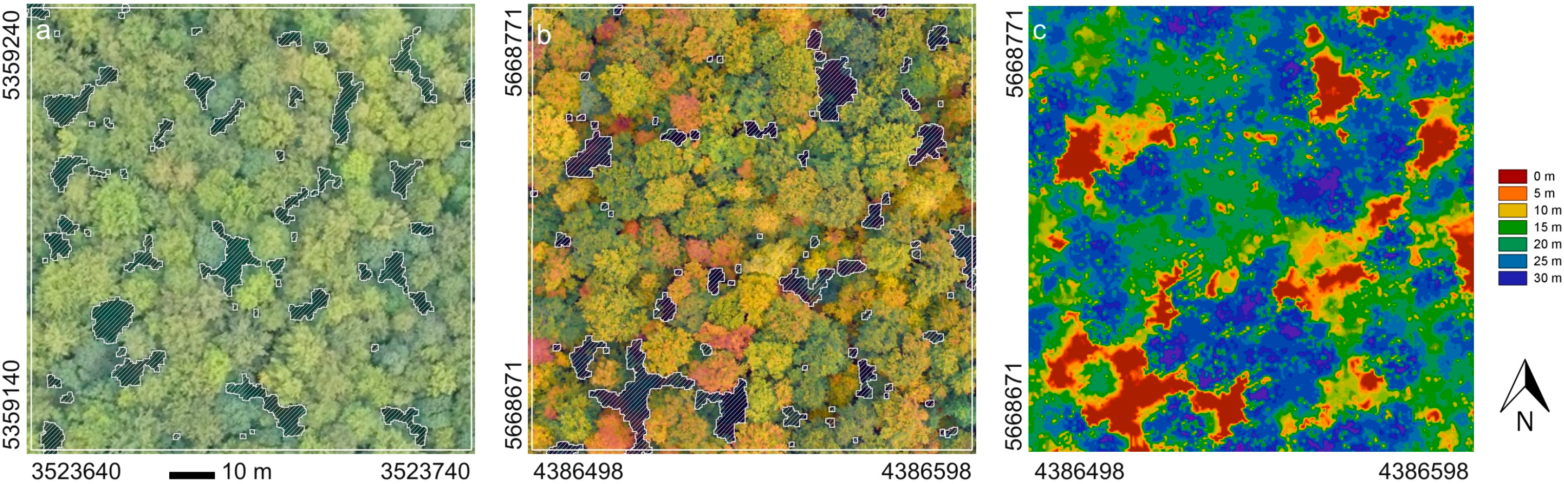
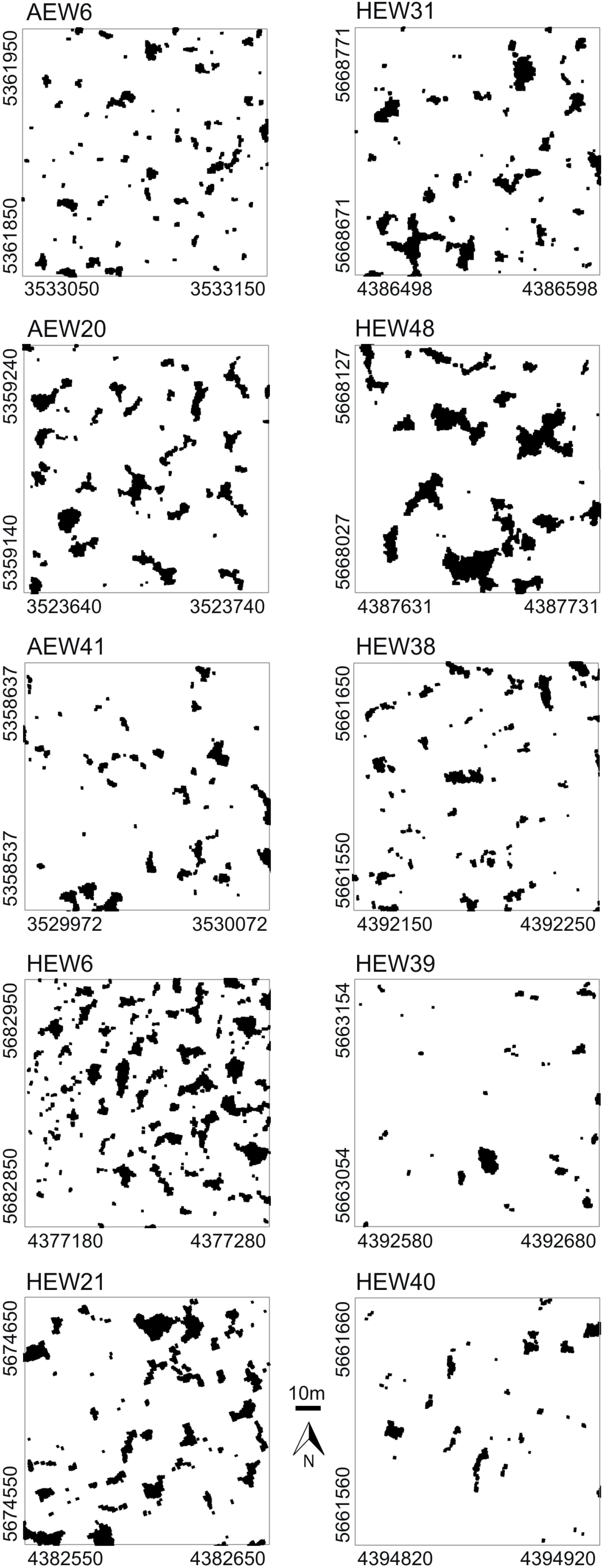
Very high-resolution RGB images (≈7 cm/pixel) were taken at the end of the summer in 2008 and 2009 with the UAV “Carolo P200” [23] above the centers of the 1-ha forest plots at flying altitudes of ≈250 m (Figure 1a,b). The UAV weighs 6 kg and has a wing span of 2 m. It can fly autonomously for a time span of 60 min along any predefined spline-based trajectory and takes an image every three seconds. All images were orthorectified based on data recordings of the internal UAV orientation, GPS position and a digital terrain model. Orthophotos were converted into binary images, and gap polygons were manually delineated as accurately as possible using ArcGIS 9.3 and saved as shapefiles (a geospatial vector data format). To assess the accuracy of our image-based method, the delineated gaps were compared to some available gap maps obtained for the same study plots with a manned LIDAR flight (Figure 1c; details in Nieschulze et al. [24]). Due to the very high image resolution, we were able to delineate gaps as small as 1 m2 in size. We segmented all gaps of a plot (Figure 2), but included in the analysis only gaps whose center of mass was inside the plot boundaries. More details can be found in Getzin et al. [5].
2.3. Spatial Statistics
We applied three spatial correlation functions for the analysis of gap distributions. At first, we used the “conventional” pair correlation function (PCF) to assess whether gap patterns were random, aggregated or regularly spaced at continuous neighborhood scales up to r = 50 m. For analyses with the conventional PCF (and the mark correlation function (MCF), see below) we used the center of mass of the gap polygons as the x,y-location. The pair correlation function g(r) is the expected density of points at a given distance r of an arbitrary point, divided by the intensity λ of the pattern [25]. The PCF is non-cumulative and, thus, particularly suitable to reveal critical scales of the pattern [26,27]. Under complete spatial randomness (CSR), g(r) = 1. Values of g(r) < 1 indicate regularity, while values of g(r) > 1 indicate aggregation.
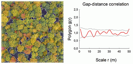
The pair correlation function is usually applied in ecology to plants, i.e., the x,y-location of the stem base, such as a tree trunk. The simplified assumption of a point-centered location is justified because the actual measurement error of the x,y-location of the stem base is approximately equal to the magnitude at which the physical size of the, for example, tree trunk may exceed the concept of the actual point measurement. For analyses of forest gaps, however, this concept appears unsuitable, because gap sizes may be very large, and the center of the gap may be far away from the gap edges. Therefore, the pair correlation function needs to be adapted to adequately deal with the real sizes and shapes of gaps [21,28]. For this purpose, we use a recently modified version of the PCF that is particularly suitable for analyzing objects of finite size and irregular shape, such as forest gaps [21]. The polygon-based pair correlation function Polygon g(r) is defined as the expected density of objects at a given distance r of an arbitrary point, divided by the intensity λ of the pattern. Since the polygon-based PCF deals with objects having a finite size, the expected number of objects under complete spatial randomness in a distance interval is difficult to determine in a closed form and even distance dependent. Thus, a correction factor is derived from the Monte Carlo simulation of the null model (see below) and subsequently applied to the estimated pair correlation function and the simulation envelopes. Distances between objects are calculated as the length of the shortest straight line between the boundary polygons. The polygon-based PCF can then be estimated as:
Finally, to quantify also the spatial distribution of gap sizes, we analyzed the gap patterns with the mark correlation function (MCF) for continuous marks [27,29]. This function does not quantify the distance correlation between gaps per se, but assesses whether there is spatial correlation between the gap sizes (area) in dependence of the gap distances r. The mark correlation function ĸmm(r) is the mean value of the test function t1(mi,mj) = mimj of the marks of two points i and j that are separated by distance r, normalized by the mean value of the test function taken over all i-j pairs in the study plot [25,26]. If the marks show no spatial correlation, we find ĸmm(r) = 1; if ĸmm(r) < 1, there is negative correlation between the marks at scale r, and if ĸmm(r) > 1, there is a positive correlation between the marks at scale r. The mark correlation function can therefore reveal if gaps that are relatively close to each other are smaller or larger than expected, given the average gap size in the plot.
Monte Carlo simulations of a homogenous Poisson process were applied for the PCF and polygon-based PCF in order to assess significant departure from the null model of complete spatial randomness. We used the fifth-lowest and fifth-highest values of 199 simulations to generate approximately 95% simulation envelopes. Note that we are here mainly interested in comparing the different functional behavior of the two PCFs and not in strict null hypothesis testing. The null model for complete spatial randomness for the polygon-based PCF was constructed by random rotation and positioning of the original objects [28]. Significant departure of the mark correlation function from the independence of the marks was similarly estimated based on random shuffling of the gap sizes.
3. Results
3.1. Structural Properties of Gaps
In the five age-class forests, the gap fraction ranged from 4.9% to 13.9%, which reflects past intensities of logging. Furthermore, the mean gap sizes were quite variable in these managed forest plots (Table 1). In our exemplary study, the five age-class forests had a larger number of gaps than the less intensively managed selection-cutting or unmanaged forests, respectively. The number of gaps for age-class forests ranged from 56 to 134 (mean = 82.6), while for the selection-cutting and unmanaged forests, it ranged from 31 to only 66 (mean = 47.2). In the selection-cutting forests of the Hainich, mean gap sizes ranged from 14 to 43 m2. These two plots had the highest maximal gap shape complexities with values of 2.7 and 2.9, respectively. In the unmanaged forest plots of the Hainich National Park, canopy gap fraction had a mean of only 3%, ranging from 2.2% to 5.7% (Table 1). Furthermore, mean gap sizes were altogether lowest in the unmanaged plots of the national park.
Overall, the proportion of very small gaps with a size <5 m2 made up on average 57.5% of all 10 forest plots with a tendency of having the largest proportion (≈65%) in the unmanaged forests (Table 1). This result is in agreement with our hypothesis.
3.2. Spatial Patterns of Gaps
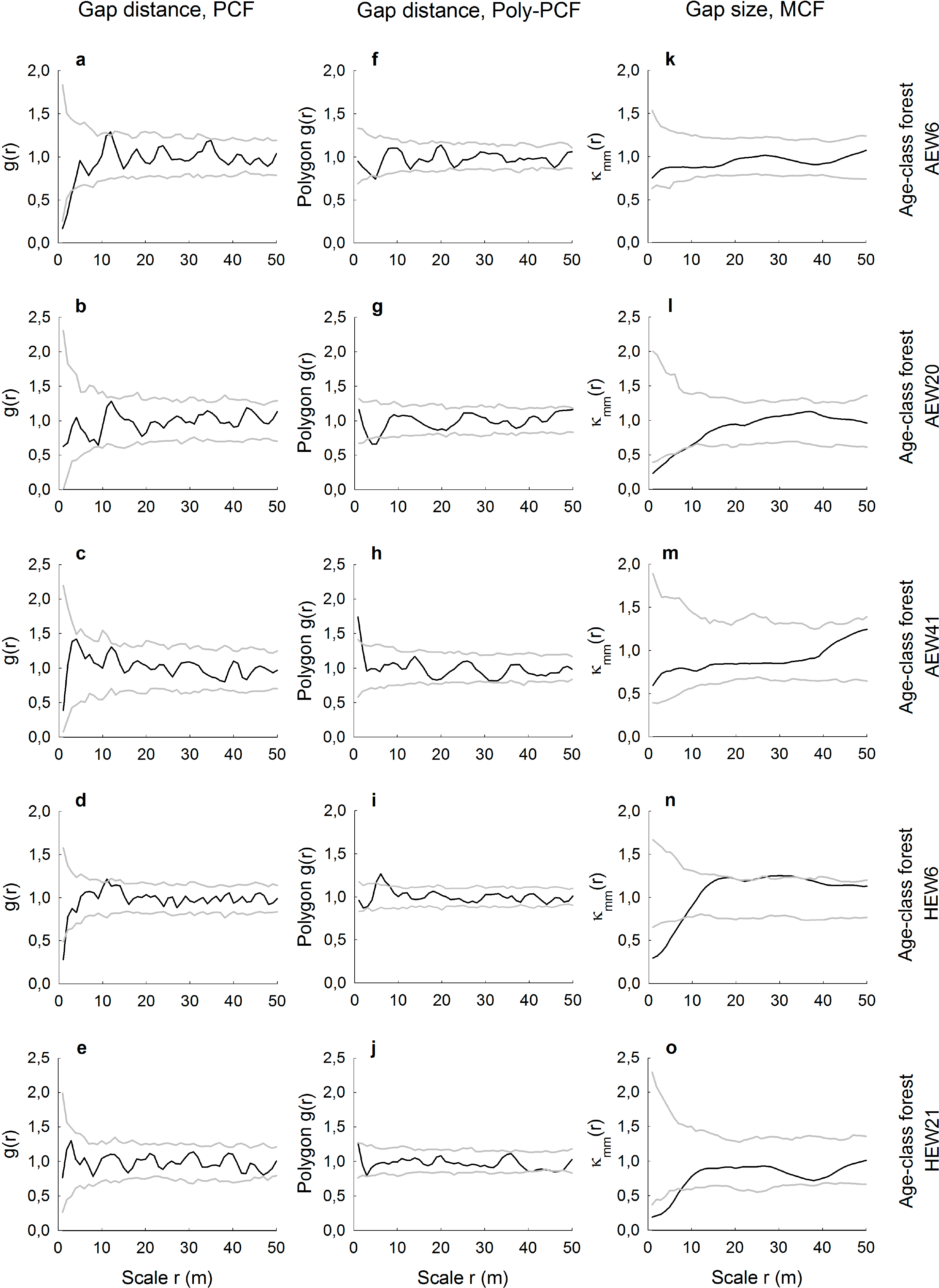
For the five age-class forests, gap distributions analyzed with the conventional pair correlation function revealed for three plots random spatial patterns and two plots small-scale regularity (Figure 3a–e). The same plots analyzed with the polygon-based PCF showed contrasting results (Figure 3f–j). For example, there was small-scale regularity (AEW20 plot) or aggregation (AEW41), even though the conventional PCF indicated randomness. In terms of indicating deviation from the null model of complete spatial randomness, results obtained with both types of pair correlation functions differed in four out of five age-class forests. There was only general agreement for the plot HEW21 (Figure 3e,j). The mark correlation function indicated for the five age-class forests that gap sizes (areas) were uncorrelated in two plots, but negatively correlated up to a maximum of 9 m in three plots (Figure 3k–o).
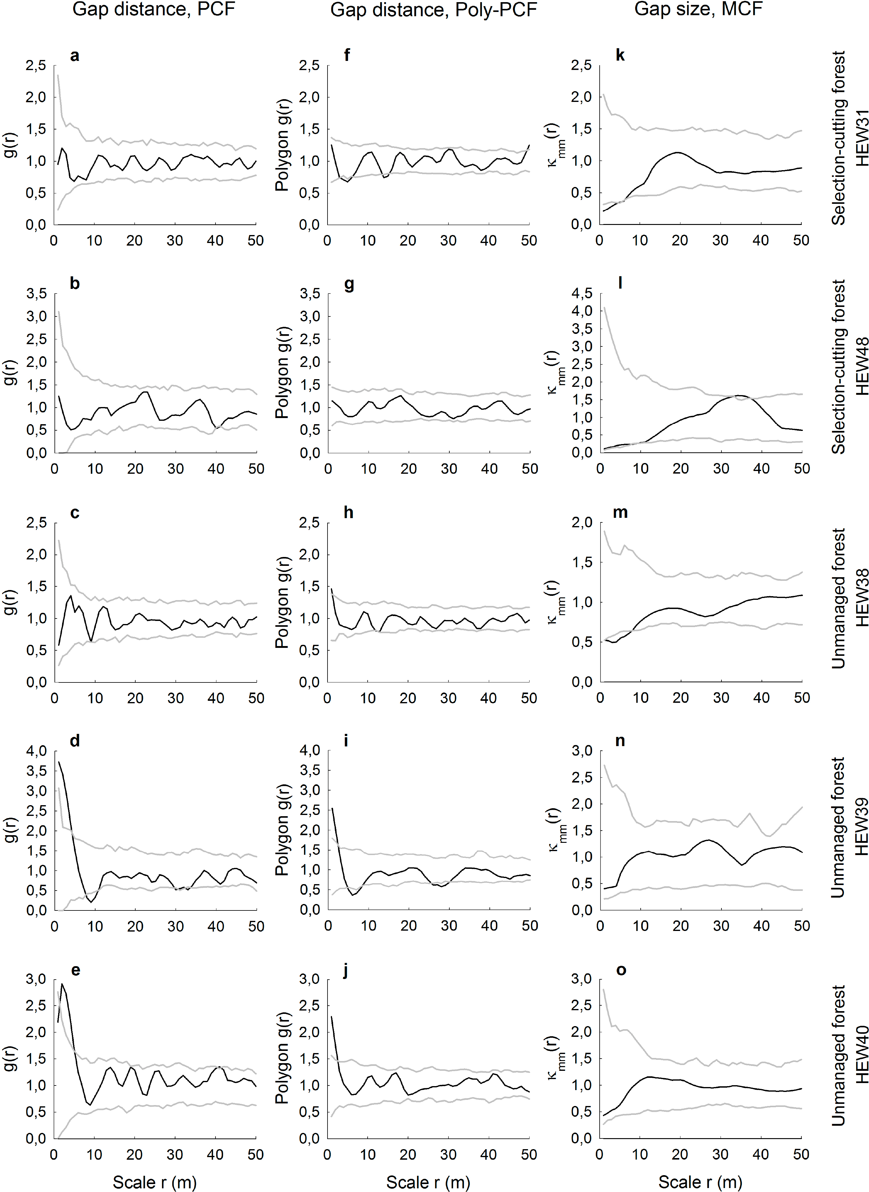
Compared to the age-class forests that had a high mean number of gaps, there was more agreement in the spatial results between the conventional and polygon-based PCFs for the selection-cutting and unmanaged forests with less numerous gaps (Figure 4a–j). Especially when gap numbers were low, i.e., ranging from 31, to 33 and 41 in the plots HEW48, HEW39 and HEW40, respectively, the conventional and the polygon-based PCFs showed a highly similar behavior. For example, gaps were aggregated at small scales in the two unmanaged forests, HEW39 and HEW40. When the gap number was higher, as in HEW31 and HEW38, differences between both types of pair correlation function were more pronounced, with the polygon-based version showing slight regularity or aggregation (Figure 4f,h) when the conventional PCF indicated no significant deviation from randomness. The mark correlation function showed only for the two plots HEW31 and HEW38 small-scale negative deviation from the null model; otherwise gap sizes were uncorrelated (Figure 4k–o).
4. Discussion
Depending on the shade-tolerance and dispersal mode of understory species, gaps are perceived either as a suitable or as non-suitable micro-habitat for regeneration, growth and survival. For example, in a study on the spatial distribution of gaps, Koukoulas and Blackburn [6,7] have shown that gaps containing mainly grass were randomly distributed at all scales, but gaps dominated by bracken (Pteridium aquilinum) were highly clustered for scales over 30 m. The dominance of bracken in clustered gaps was due to its vegetative spread via below-ground rhizomes, which creates large contiguous patches across gaps where tree regeneration is severely inhibited. This demonstrates that the horizontal pattern of gaps in the canopy layer is a fine-scale spatial structure that influences the recruitment success of understory individuals [8]. The scale-dependent functional connectivity of the gap locations is therefore one of the drivers for tree recruitment and understory biodiversity in forests [5,15,34]. However, since the scale at which individuals perceive and interact with canopy structures depends on the species, it needs to be identified by testing for a correlation between population-dynamic features of interest and structural characteristics at different spatial scales [12]. Doing so, knowledge of the gap distribution pattern can thus be used either to better understand successional dynamics and changes of biodiversity in forests or to actively influence and control those dynamics via silvicultural prescriptions and rules for spatial tree retention and gap creation.
So far, the spatial distribution of gaps has seldom been quantified in a spatially-explicit manner (but see [7,21,35]). One obvious reason for this is that terrestrial mapping of the patterns of gaps is very time-consuming and, thus, done rarely on continuous neighborhood scales. Another reason is that the resolution of conventional aerial (20 cm/pixel) or satellite images (≥50 cm/pixel) is too coarse to permit delineating gaps as small as 1 m2. However, some ecological phenomena, such as the canopy-structural dependencies of certain understory species, are only observable at small scales and, hence, only quantifiable if enough gaps would contribute to the small-scale spatial pattern analysis. Here is the advantage of using unmanned aerial vehicles for the mapping of gaps. Images taken at low flying altitudes have such a high resolution (usually <10 cm/pixel), that minimal gap sizes of 1 m2 and their shape can be safely mapped and included in the data set for assessing gap distributions. This inclusion of the smallest gaps will not only lead to a sufficient sample size to permit spatially-explicit analyses, but also, to new possibilities of ecological inference.
As to the definition of gaps, others have identified minimal gap sizes of 5 m2 using airborne LIDAR information, but this size was “chosen arbitrarily” [17] and does not reflect vegetation response to certain threshold values of minimal gap sizes. In fact, there is as yet no rule based on ecological mechanisms to decide whether gap recordings should be restricted to thresholds of 5 m2 or 1 m2. This is because research on revealing the ecological importance of very small gaps is so far relatively rare. Nieschulze et al. [24] have, for example, extracted gaps with LIDAR for some of the same forest plots used here, but they have not defined a typical minimum size limit or the cause of the canopy openings. Likewise, Boyd et al. [16] used LIDAR data to identify smallest gap sizes of 1 m2 for a 24-km2 area in tropical Peru. They further investigated the smallest gap sizes up to 2 m2 for an extended landscape of more than 140 km2 and found that small gaps dominated, while those gaps being larger than 100 m2 made up only 0.45% of all documented canopy openings. Overall, there seems to be a trend that, with the availability of increasingly higher 2D or 3D image resolutions, gap definitions are being adapted to suit the emphasis on spatial phenomena and light-dependent processes that could not be analyzed previously.
Here, we found evidence in support of our hypothesis (and in overall agreement with the results of Boyd et al. [16]): the very small gaps of a size <5 m2 made up the largest proportion of all gaps found in the study plots. This was particularly the case for the three unmanaged forests where gaps are naturally induced, mainly by disturbance. Indeed, very small gaps may also be important for forest dynamics. Very small gaps belong often to repeated gaps that occur along the edges of old gaps. They are primarily formed by the lateral expansion of branches following the destruction of these branches. Torimaru et al. [36] have demonstrated that most repeated gaps were smaller than 10 m2 in deciduous and coniferous forests and that “future analyses […] should pay attention to repeated gap formation events and their spatial patterns”. While we have not analyzed aerial images in consecutive years, it is quite likely that the very small gaps detected here are part of repeated gap formation induced by small-scale disturbance. For example, trees of gap peripheries are more vulnerable to mortality and injury than interior canopy trees, which could lead to small openings [37]. Overall, it has been shown that repeated disturbances are important for the regeneration of species that can tolerate intermediate light levels and that are able to survive several periods of suppression from neighboring trees before growing into the canopy [38]. So far, small gaps are often neglected in forest studies, but they are also structural drivers for forest dynamics. With reference to the traditional framework for studies of forests based on schematic gap dynamics and discrete phases from gaps to mature forest, Torimaru et al. [36] emphasize that “repeated gap-creating disturbances commonly occur, so schematic gap dynamics do not always provide realistic descriptions of forest dynamics”. Furthermore, Tanaka and Nakashizuka [39] found a high probability of repeated gap disturbance for a deciduous temperate forest, and they postulated that the “high occurrence of disturbances around the existing gaps should not be explained simply as gap expansion, but should be considered an important factor in canopy dynamics”. We agree with these statements and recommend that more studies should be undertaken to quantify repeated gap formation and the spatial patterns. It would be especially interesting to link in consecutive years of monitoring the spatial patterns of gaps to regeneration and successional dynamics in the understory. This will help to better understand the relative importance of traditionally recorded larger gaps vs. the ecological importance of small repeated gaps.
In our study, we included gap sizes as small as 1 m2, because these smallest gaps are important determinants of regeneration, since the variability of diffuse radiation does influence understory biodiversity [15]. The importance of such fine-scale information on the spatially-implicit properties of gaps, including detailed descriptions on their shape complexity, has recently been demonstrated for determining understory biodiversity in temperate forests [5]. However, also in tropical forests, the fine-scale properties of gaps may be important drivers of understory vegetation. For example, Montgomery and Chazdon [14] have shown that the growth of tropical tree seedlings in low light environments is highly sensitive to light availability and that shade-tolerant species vary in these responses. Thus, very small gaps causing light heterogeneity in the understory may induce light-gradient partitioning and affect recruitment processes for shade-tolerant tree species.
We demonstrated how spatially-explicit, i.e., scale-dependent, information on gap distributions can be extracted from very high-resolution images. Pair and mark correlation functions have the ability to quantify positive or negative distance and size correlations, respectively, for a continuous range of neighborhood scales. However, we have shown that it may depend on the type of pair correlation function used whether gap patterns may be random, regularly distributed or aggregated. The conventional PCF is based on the point approximation and, thus, measures the distances between centroids of the gaps. This may lead to the indication of the small-scale regularity of the centroids in cases where gaps are indeed randomly distributed, because the physical size and shape of the gaps prevent measuring short neighborhood distances. Such unwanted artifacts in the PCF resembling a so-called “soft-core process” have been shown for artificial data [21], but are also visible in our real data. For example, it is likely that the gaps in the plots AEW6 and HEW6 are not regularly spaced at smallest scales up to approximately r = 3 m, but are, rather, random at that scale (Figure 3f,i). This is because the polygon-based PCF provides information about the distribution of distances from the boundary of a gap to the edge of another gap and, thus, measures the space between the gaps. While the conventional PCF could partly account for that with a special soft-core null model, the approach of the polygon-based PCF is much more straightforward. Furthermore, we found that differences between the conventional and the polygon-based PCF were smallest when the number of gaps per plot was very low, such as in the two unmanaged plots of the Hainich National Park. This could indicate that the likelihood of biasing effects from soft-core processes becomes smaller when there are relatively few gaps in a plot. The agreement or disagreement between both PCF versions does also depend on the size and the actual shape of the gaps, i.e., whether the shape eccentricity causes large deviations between distance measurements of gap centers vs. gap boundaries.
More robust against these problems of physical object sizes in spatially-explicit analyses is the use of the mark correlation function. The MCF is typically applied to, for example, the diameters of tree trunks [29], but it has also been recently used to assess the size correlation of tree crowns [26]. However, application of the MCF to forest gaps seems to be a novel approach. Here, we found that gap sizes were in five plots independent of scale and in another fives plots negatively correlated at small neighborhood scales up to a maximum of 9 m. The absence of positive size correlations indicates that particularly large gaps with above-average size never occurred in clusters. Otherwise, four of the five negative gap-size correlations occurred in managed plots. This may reflect tree retention patterns and the spatial signature of thinning carried out by the forester. For example, small gaps with below-average sizes may be relatively close to each other when the forester undertakes single-tree harvests or removes thin trees or trees of low crown vitality around preferred target trees [10].
Overall, we want to emphasize that our comparison of gap structures and spatial patterns in differently managed forests can only be viewed as a first exemplary study. In order to allow more thorough insights on gap dynamics evolving under different land-use intensities, larger datasets need to be sampled to permit generalizations.
From a technical point of view, we recommend undertaking UAV flights only under relatively cloudy conditions without direct sunlight. Such diffuse sky radiation will help to avoid misclassifications of gaps caused by the hard shadows of neighboring trees, which would appear as dark patches. In our study, we have avoided such unwanted effects and were thus able to delineate the gaps accurately so that they matched the gaps recorded with a manned LIDAR flight (cf. Figure 1). Furthermore, we recommend undertaking flights, especially with rotary-wing UAVs, rather under calm wind conditions, so that the UAV system will remain horizontally stable (roll and pitch angles) while photographing gaps. This is required, because for spatially-explicit gap analyses, as undertaken here, forest images need to be well orthorectified, so that all gap locations and their distances between them are up to scale.
5. Conclusions
Unmanned aerial vehicles are highly suitable tools for mapping small gaps, repeated gap formation and spatial canopy structures in general. With our study, we have shown that they provide not only very high-resolution images to record gap openings as small as 1 m2 [5], but they can be used very flexibly for monitoring purposes [18]. For example, the low monetary costs required for a flight mission with a UAV makes it possible to record the spatial dynamics of repeated gap formation on an annual basis. Spatially-explicit analyses, such as applied here, can be used to monitor the change in distance and size correlation of gaps. These changes can then be related either to the initial state of tree-harvesting patterns in managed forests or to the successional dynamics of the understory in unmanaged forests. With our unique study, which applied for the first time UAV technology in combination with spatially-explicit gap analyses, we have demonstrated how gap patterns can be related to the spatio-temporal dynamics of forests. Of course, as UAVs and their on-board sensors are currently rapidly advancing, new technology will soon allow even higher image resolutions and more refined canopy segmentations. Furthermore, as portable payloads on UAVs are constantly increasing, new sensors, such as LIDAR for 3D mapping of gaps, will become more common in such applications. Successful trials with LIDAR sensors attached to UAVs have been already undertaken [40,41], and additional information on true canopy height will allow even more accurate gap mappings in the near future.
Acknowledgments
We thank the managers of the three exploratories, Swen Renner, Sonja Gockel, Kerstin Wiesner and Martin Gorke, for their work in maintaining the plot and project infrastructure; Simone Pfeiffer and Christiane Fischer for giving support through the central office; Michael Owonibi for managing the central database; and Markus Fischer, Eduard Linsenmair, Dominik Hessenmöller, Jens Nieschulze, Daniel Prati, Ingo Schöning, François Buscot, Ernst-Detlef Schulze, Wolfgang W. Weisser and the late Elisabeth Kalko for their role in setting up the Biodiversity Exploratories project. Field work permits were issued by the responsible state environmental offices of Baden-Württemberg, Thüringen and Brandenburg (according to § 72 BbgNatSchG). The authors are grateful to the developers of the UAV, such as Sergej Chmara, Herbert Sagischewski, Marco Buschmann, Lars Krüger and Thomas Krüger from the Andromeda-Project and the Institute of Aerospace Systems/TU Braunschweig. The study was funded by the DFG Priority Program 1374 “Infrastructure-Biodiversity-Exploratories” (WI 1816/9-1), and Stephan Getzin was also supported by the European Research Council (ERC) Advanced Grant “SpatioDiversity” (grant number 233066). We want to thank three reviewers for their constructive criticism.
Author Contributions
Stephan Getzin proposed the study, acquired the data, supervised the canopy gap delineation, analyzed the canopy gap patterns using the traditional pair correlation function and the mark correlation function, interpreted the results and wrote the manuscript. Robert Nuske analyzed the patterns using the polygon-based pair correlation function, interpreted the results and contributed in manuscript writing and revision. Kerstin Wiegand advised on the study design and interpretation and contributed to manuscript writing and revision.
Conflicts of Interest
The authors declare no conflict of interest.
References
- Augusto, L.; Dupouey, J.-L.; Ranger, J. Effects of tree species on understory vegetation and environmental conditions in temperate forests. Ann. For. Sci 2003, 60, 823–831. [Google Scholar]
- Boch, S.; Prati, D.; Müller, J.; Socher, S.; Baumbach, H.; Buscot, F.; Gockel, S.; Hemp, A.; Hessenmöller, D.; Kalko, E.K.V.; et al. High plant species richness indicates management-related disturbances rather than the conservation status of forests. Basic Appl. Ecol 2013, 14, 496–505. [Google Scholar]
- Proulx, R.; Parrott, L. Measures of structural complexity in digital images for monitoring the ecological signature of an old-growth forest ecosystem. Ecol. Indic 2008, 8, 270–284. [Google Scholar]
- Mountford, E.P.; Savill, P.S.; Bebber, D.P. Patterns of regeneration and ground vegetation associated with canopy gaps in a managed beechwood in southern England. Forestry 2006, 79, 389–408. [Google Scholar]
- Getzin, S.; Wiegand, K.; Schoning, I. Assessing biodiversity in forests using very high-resolution images and unmanned aerial vehicles. Methods Ecol. Evol 2012, 3, 397–404. [Google Scholar]
- Koukoulas, S.; Blackburn, G.A. Quantifying the spatial properties of forest canopy gaps using LiDAR imagery and GIS. Int. J. Remote Sens 2004, 25, 3049–3071. [Google Scholar]
- Koukoulas, S.; Blackburn, G.A. Spatial relationships between tree species and gap characteristics in broad-leaved deciduous woodland. J. Veg. Sci 2005, 16, 587–596. [Google Scholar]
- Kuuluvainen, T.; Linkosalo, T. Estimation of a spatial tree-influence model using iterative optimization. Ecol. Model 1998, 106, 63–75. [Google Scholar]
- Drever, C.R.; Lertzman, K.P. Effects of a wide gradient of retained tree structure on understory light in coastal Douglas-fir forests. Can. J. For. Res 2003, 33, 137–146. [Google Scholar]
- Battaglia, M.A.; Mou, P.; Palik, B.; Mitchell, R.J. The effect of spatially variable overstory on the understory light environment of an open-canopied longleaf pine forest. Can. J. For. Res 2002, 32, 1984–1991. [Google Scholar]
- Coates, K.D.; Canham, C.D.; Beaudet, M.; Sachs, D.L.; Messier, C. Use of a spatially explicit individual-tree model (SORTIE/BC) to explore the implications of patchiness in structurally complex forests. For. Ecol. Manag 2003, 186, 297–310. [Google Scholar]
- Wiegand, T.; Moloney, K.A.; Naves, J.; Knauer, F. Finding the missing link between landscape structure and population dynamics: A spatially explicit perspective. Am. Nat 1999, 154, 605–627. [Google Scholar]
- Ramirez, F.A.; Armitage, R.P.; Danson, F.M. Testing the application of terrestrial laser scanning to measure forest canopy gap fraction. Remote Sens 2013, 5, 3037–3056. [Google Scholar]
- Montgomery, R.A.; Chazdon, R.L. Light gradient partitioning by tropical tree seedlings in the absence of canopy gaps. Oecologia 2002, 131, 165–174. [Google Scholar]
- Moora, M.; Daniell, T.; Kalle, H.; Liira, J.; Püssa, K.; Roosaluste, E.; Öpik, M.; Wheatley, R.; Zobel, M. Spatial pattern and species richness of boreonemoral forest understorey and its determinants—A comparison of differently managed forests. For. Ecol. Manag 2007, 250, 64–70. [Google Scholar]
- Boyd, D.S.; Hill, R.A.; Hopkinson, C.; Baker, T.R. Landscape-scale forest disturbance regimes in southern Peruvian Amazonia. Ecol. Appl 2013, 23, 1588–1602. [Google Scholar]
- Vepakomma, U.; St-Onge, B.; Kneeshaw, D. Spatially explicit characterization of boreal forest gap dynamics using multi-temporal lidar data. Remote Sens. Environ 2008, 112, 2326–2340. [Google Scholar]
- Anderson, K.; Gaston, K.J. Lightweight unmanned aerial vehicles will revolutionize spatial ecology. Front. Ecol. Environ 2013, 11, 138–146. [Google Scholar]
- Koh, L.P.; Wich, S.A. Dawn of drone ecology: Low-cost autonomous aerial vehicles for conservation. Trop. Conserv. Sci 2012, 5, 121–132. [Google Scholar]
- Wing, M.G.; Burnett, J.; Sessions, J.; Brungardt, J.; Cordell, V.; Dobler, D.; Wilson, D. Eyes in the sky: Remote sensing technology development using small unmanned aircraft systems. J. For 2013, 111, 341–347. [Google Scholar]
- Nuske, R.S.; Sprauer, S.; Saborowski, J. Adapting the pair correlation function for analysing the spatial distribution of canopy gaps. For. Ecol. Manag 2009, 259, 107–116. [Google Scholar]
- Fischer, M.; Bossdorf, O.; Gockel, S.; Hansel, F.; Hemp, A.; Hessenmöller, D; Korte, G.; Nieschulze, J.; Pfeiffer, S.; Prati, D.; et al. Implementing large-scale and long-term functional biodiversity research: The biodiversity exploratories. Basic Appl. Ecol 2010, 11, 473–485. [Google Scholar]
- Böhm, B.; Böhm, C.; Chmara, S.; Flügel, W.-A.; Krüger, T.; Neumann, M.; Reinhold, M.; Sagischewski, H.; Selsam, P.; Vörsmann, P.; Wilkens, C.-S. ANDROMEDA—Mapping of forest calamities by unmanned aerial vehicles—From vision to productive process. Forst Holz 2008, 63, 37–42. [Google Scholar]
- Nieschulze, J.; Zimmermann, R.; Börner, A.; Schulze, E.D. An assessment of forest canopy structure by LiDAR: Derivation and stability of canopy structure parameters across forest management types. Forstarchiv 2012, 83, 195–209. [Google Scholar]
- Illian, J.; Penttinen, A.; Stoyan, H.; Stoyan, D. Statistical Analysis and Modelling of Spatial Point Patterns; John Wiley & Sons: Chichester, UK, 2008. [Google Scholar]
- Getzin, S.; Wiegand, K.; Schumacher, J.; Gougeon, F.A. Scale-dependent competition at the stand level assessed from crown areas. For. Ecol. Manag 2008, 255, 2478–2485. [Google Scholar]
- Stoyan, D.; Stoyan, H. Fractals, Random Shapes and Point Fields: Methods of Geometrical Statistics; John Wiley & Sons: Chichester, UK, 1994. [Google Scholar]
- Wiegand, T.; Kissling, W.D.; Cipriotti, P.A.; Aguiar, M.R. Extending point pattern analysis for objects of finite size and irregular shape. J. Ecol 2006, 94, 825–837. [Google Scholar]
- Penttinen, A.; Stoyan, D.; Henttonen, H.M. Marked point-processes in forest statistics. For. Sci 1992, 38, 806–824. [Google Scholar]
- Ripley, B.D. Spatial Statistics; John Wiley & Sons: New York, NY, USA, 1981. [Google Scholar]
- GEOS—Geometry Engine Open Source. Available online: http://trac.osgeo.org/geos (accessed on 4 May 2014).
- PostGIS. Available online: http://postgis.net (accessed on 4 May 2014).
- R Development Core Team. R: A Language and Environment for Statistical Computing; R Foundation for Statistical Computing: Vienna, Austria, 2013. [Google Scholar]
- Tinya, F.; Marialigeti, S.; Kiraly, I.; Nemeth, B.; Odor, P. The effect of light conditions on herbs, bryophytes and seedlings of temperate mixed forests in Őrség, Western Hungary. Plant Ecol 2009, 204, 69–81. [Google Scholar]
- Petritan, A.N.; Nuske, R.S.; Petritan, I.C.; Tudose, N.C. Gap disturbance patterns in an old-growth sessile oak (Quercus petraea L.)—European beech (Fagus sylvatica L.) forest remnant in the Carpathian Mountains, Romania. For. Ecol. Manag 2013, 308, 67–75. [Google Scholar]
- Torimaru, T.; Itaya, A.; Yamamoto, S.I. Quantification of repeated gap formation events and their spatial patterns in three types of old-growth forests: Analysis of long-term canopy dynamics using aerial photographs and digital surface models. For. Ecol. Manag 2012, 284, 1–11. [Google Scholar]
- Vepakomma, U.; Kneeshaw, D.; St-Onge, B. Interactions of multiple disturbances in shaping boreal forest dynamics: A spatially explicit analysis using multi-temporal lidar data and high-resolution imagery. J. Ecol 2010, 98, 526–539. [Google Scholar]
- Runkle, J.R.; Yetter, T.C. Treefalls revisited—Gap dynamics in the southern Appalachians. Ecology 1987, 68, 417–424. [Google Scholar]
- Tanaka, H.; Nakashizuka, T. Fifteen years of canopy dynamics analyzed by aerial photographs in a temperate deciduous forest, Japan. Ecology 1997, 78, 612–620. [Google Scholar]
- Lin, Y.; Hyyppä, J.; Jaakkola, A. Mini-UAV-borne LIDAR for finescale mapping. IEEE Geosci. Remote Sens.Lett 2011, 8, 426–430. [Google Scholar]
- Wallace, L.; Lucieer, A.; Watson, C.; Turner, D. Development of a UAV-LiDAR system with application to forest inventory. Remote Sens 2012, 4, 1519–1543. [Google Scholar]


| Plot (Management Type) | # of Gaps | Gap Fraction (%) | Gap Size (m2) Mean/Max | % gaps <5 m2 | GSCI Mean/Max |
|---|---|---|---|---|---|
| AEW6 (age class) | 88 | 5.6 | 6.4/39.7 | 64.8 | 1.3/2.1 |
| AEW20 (age class) | 56 | 9.8 | 17.5/81.7 | 42.9 | 1.5/2.4 |
| AEW41 (age class) | 56 | 4.9 | 8.7/50.7 | 55.4 | 1.3/2.0 |
| HEW6 (age class) | 134 | 13.9 | 10.4/73.2 | 63.4 | 1.4/2.5 |
| HEW21 (age class) | 79 | 12.0 | 15.2/150.0 | 51.9 | 1.4/2.4 |
| HEW31 (selection cutting) | 65 | 9.2 | 14.1/163.5 | 60.0 | 1.4/2.9 |
| HEW48 (selection cutting) | 31 | 13.4 | 43.3/244.0 | 41.9 | 1.6/2.7 |
| HEW38 (unmanaged) | 66 | 5.7 | 8.6/65.0 | 59.1 | 1.4/2.3 |
| HEW39 (unmanaged) | 33 | 2.2 | 6.6/64.5 | 69.7 | 1.3/1.7 |
| HEW40 (unmanaged) | 41 | 2.8 | 6.9/39.9 | 65.9 | 1.3/2.1 |
© 2014 by the authors; licensee MDPI, Basel, Switzerland This article is an open access article distributed under the terms and conditions of the Creative Commons Attribution license (http://creativecommons.org/licenses/by/3.0/).
Share and Cite
Getzin, S.; Nuske, R.S.; Wiegand, K. Using Unmanned Aerial Vehicles (UAV) to Quantify Spatial Gap Patterns in Forests. Remote Sens. 2014, 6, 6988-7004. https://doi.org/10.3390/rs6086988
Getzin S, Nuske RS, Wiegand K. Using Unmanned Aerial Vehicles (UAV) to Quantify Spatial Gap Patterns in Forests. Remote Sensing. 2014; 6(8):6988-7004. https://doi.org/10.3390/rs6086988
Chicago/Turabian StyleGetzin, Stephan, Robert S. Nuske, and Kerstin Wiegand. 2014. "Using Unmanned Aerial Vehicles (UAV) to Quantify Spatial Gap Patterns in Forests" Remote Sensing 6, no. 8: 6988-7004. https://doi.org/10.3390/rs6086988