1. Introduction
Electronic path delays, oscillator drifts, time tagging errors, antenna phase centre uncertainties, orbit errors, errors in geophysical correction models, improperly calibrated auxiliary sensors and even software conventions may cause systematic errors of the altimeter range (the distance from the satellite to the instantaneous sea level), the most important parameter to monitor the global and regional sea level evolution. On average these errors include a constant range bias, a drift term or even geographically correlated error pattern all of them mapping directly to the sea surface heights. This underpins the importance of a careful calibration of satellite based altimeter systems. A calibration is an indispensable prerequisite to construct a long-term data record to investigate sea level rise and to study regional sea level variability.
The range bias (and eventually, the drift term) can be estimated by a calibration scenario in which the altimeter derived sea surface heights are compared (over a sufficient long period of time) with geocentric sea level heights derived independently, e.g., by GPS-linked tide gauges or GPS equipped buoys. In the last two decades several permanent sites have been set up providing
absolute. Yes, the reader should become aware of the differences between absolute and relative calibration calibration of satellite altimeters. Without claiming to be complete, some of these sites are located in Europe (Corsica in France [
1], Gavdos in Greece [
2]) in the USA (Harvest Oil Platform, California, [
3]) or in Australia (Bass Strait, Tasmania [
4]).
For TOPEX (Ocean TOPography EXperiment), an absolute calibration procedure was first realized at the Harvest Platform. Up to now, the approach has been applied systematically for every 10-day repeat cycle for the full lifetime of the NASA/CNES (National Aeronautics and Space Administration/Centre National d’Etudes Spatiales) missions TOPEX/Poseidon and the follow-on missions Jason-1 and Jason-2 [
5,
6], all of them operating over the same ground tracks. On several sites at Corsica, point calibrations are not only performed for the NASA/CNES missions, but also for the European Space Agency (ESA) missions, ERS-2 (2nd Earth Remote Sensing satellite) and ENVISAT (ENVIronmental SATellite), as well as for SARAL (SAtellite for ARgos and ALtiKa) [
7,
8]. Instantaneous bias estimates are obtained by comparing GPS buoy sea level measurements and tide gauge recordings with altimeter observations. A ground track of the NASA/CNES missions is also captured by the calibration site in Bass Strait and at Storm Bay (Tasmania) [
9]. This site has also been operated since the launch of TOPEX/Poseidon and now combines GPS buoys, ocean moorings and tide gauge observation. The Gavdos-site (south of Creta), located under a crossing of TOPEX/Jason ascending and descending tracks, has been operated since 2004 [
2]. It facilitates GPS linked tide gauges, satellite tracking instruments and an active microwave transponder for the radar altimeters [
10]. Recently, [
11] introduced a regional calibration approach, claiming to be comparable to the absolute calibration estimates of
in situ sites. It relies on a succession of mean sea surface profiles by which several missions can be combined. This way, a first absolute calibration of ENVISAT was achieved by using the environment of Harvest and Corsica
in situ sites.
Not all missions (or sequence of missions with identical orbit configuration) have been calibrated with a comparable rigour. Initially, ERS-1 (1st Earth Remote Sensing satellite) was calibrated only by a few overflights of an oil platform near Venice [
12] and later on by a short-arc calibration with
in situ data in the English Channel [
13]. Compared to the NASA/CNES missions, the orbit of ERS-1 was also degraded due to the failure of PRARE (Precise Range And Range rate Experiment), a microwave tracking system. This was the rationale for a cross-calibration approach aiming to improve the ERS-1 orbit using TOPEX as a reference and estimating the relative range bias of ERS-1 w.r.t TOPEX [
14]. Later on this relative calibration w.r.t TOPEX was also applied to other missions as well, e.g., by [
15].
ERS-2 had a few months of overlap operation with ERS-1, allowing the observation of identical sea surface height profiles with a delay of one day. Such formation flight configurations were also realized for the transition from ERS-2 to ENVISAT (30 min ahead of ERS-2), from TOPEX to Jason-1 and from Jason-1 to Jason-2 (with a delay of only 60 s) lasting each several months. With decreasing time difference, the measurement conditions of a formation flight become similar, such that sea level variability and sea state (wave heights) conditions cancel each other efficiently. These repeat pass analyses allow the most direct comparison of sea surface heights and provide rather small error estimates. On the other hand the relative calibration by repeat pass analyses is critical, as undetected drifts of the primary mission are projected to the follow-on mission.
However, also, the absolute
in-situ calibrations at fixed sites are not without problems. These sites should be far enough from land to avoid a contamination of the altimeter signal. They should be also small enough such that the site will not affect the altimeter response. These condition are best fulfilled by the Harvest platform. Tide gauge comparisons always require extrapolations from open sea towards the coastal site by means of mean sea level or the geoid. Indeed, mean range bias estimates of Harvest, Corsica, Gavdos, and the Bass Strait are not absolutely consistent and may differ by 20 mm even if processing strategies are rather consistent; see, for example, [
7]. Geographically correlated errors or site-specific environmental conditions could be an explanation for the remaining discrepancies addressed by [
7]. Long-term changes of altimeter range and geophysical corrections at altimeter calibration site were recently investigated by [
16].
GPS equipped buoys provide another tool to directly measure the instantaneous sea surface height in the geocentric terrestrial reference system. This was e.g., applied for ERS-1 in the North Sea [
17] and for TOPEX/Poseidon at the Harvest site [
18]. Waveride buoys (a floater design) were used for TOPEX calibration in the Galveston Bay [
19,
20]. Later on [
21] conducted a GPS buoy campaign in Lake Erie. In order to obtain by GPS buoys geocentric sea surface heights with sufficient precision, near-by reference sites are required for differential GPS processing.
A comparison with global tide gauge networks have been proven to identify possible drifts and bias instabilities of altimeter systems over time [
22]. The rationale of this comparison is that the differences between tide gauge records and time series of altimetric sea surface heights should not exhibit any drift or systematic offset over sufficient long periods of time. The geographical distribution of tide gauges may not be optimal and their records may contain regional sea level variations not representative for the whole globe. However, by this method, an early drift in the TOPEX, Side A, altimeter system could be detected [
22]. Using satellite altimetry for sea level rise studies is essential to verfiy that the systems are free from significant drifts [
23]. In relative calibration approaches drifts are not visible by those altimeter system used as reference. This underpins the importance of cross-calibrating altimeter systems with tide gauges.
The approach presented here is a
relative calibration and provides only relative range biases with respect to NASA/CNES reference missions (which have, due to three independent tracking systems, the most robust orbital ephemeris and benefit from the continuous absolute calibration at the
in situ calibration sites mentioned above). However, in contrast to a one-by-one cross-calibration of pairs of missions (e.g., [
14] for ERS1/2 and TOPEX, or [
15] for ENVISAT and Jason1/2) the present approach is applied in a
multi-mission scenario. This scenario automatically includes the repeat-pass analysis of formation flights. Single- and dual-satellite crossovers are used in all combinations, generating a highly redundant network. This allows a robust estimation of time series of radial errors for the full lifetime of all missions. Subsequently, the stochastic properties of the altimeter ranges can be characterized and systematic errors can be quantified.
At this point, it should be already emphasized that all (residual) errors of correction models for sea state, radiometer, tides etc. map to the crossover differences just as errors in realizing the reference system or errors mapping to the orbit due to residual gravity field uncertainties. Therefore we speak nearly exceptionally of “radial errors” (not only of “orbit errors”) and mean that the estimated errors represent an overall error of the altimeter system.
The present paper is structured as follows: The comprehensive multi-mission altimeter data base used for the cross-calibration is described first, along with the efforts to gradually upgrade and harmonize the data. Section 3 explains in detail the cross-calibration methodology in terms of discrete modelling of radial errors, the treatment of multi-mission scenarios and the numerics applied to solve the least squares adjustment of a rather huge systems. Section 4 presents selected details of the extensive results of a multi-mission cross calibration for all altimeter systems operating the past two decades in order to indicate the specific potential of the approach presented here. The final conclusions summarizes the particular findings of the multi-mission cross-calibration.
2. Altimeter Data Holdings
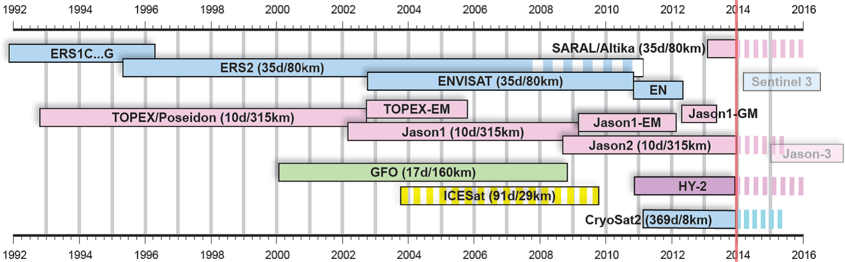
Since the launch of TOPEX/Poseidon in 1992 at least two altimetry missions provide highly accurate contemporaneous measurements of the sea surface. In the last two decades data of 12 different altimeters were acquired, in some time periods, up to six missions were operated simultaneously.
Figure 1 illustrates the altimeter mission history of the last two decades.
The approach presented here not only rely on the so-called core missions (TOPEX and Jason-1/2) flying continuously on a fixed orbit with a repeat cycle of about 10 days. It also includes the ESA missions ERS1/2 and ENVISAT providing a denser ground track pattern with a 35 days repeat cycle and GFO (Geosat Follow-On) with 17 days repeat. In addition, this investigation also uses missions with very long repeat cycles, such as ERS-1 geodetic mission (GM) phases, Cryosat-2 LRM (Low Rate Mode) from ESA Baseline B and Jason-1 GM (completing a full geodetic mission phase just before its end-of-life). Even satellites with drifting orbits (ENVISAT extended mission (EM)) as well as the episodic laser altimeter measurements provided by ICESat (Ice, Cloud, and land Elevation Satellite) (Release 33) [
24] are included in the cross-calibration. Recently, the IGDR-data (Interim Geophysical Data Record) from HY-2A (HaiYang satellite 2A) and GDR-T-data (Geophysical Data Record, version T, patch1) of SARAL complemented the commonly analyzed data. Some of the missions are separated into different sub-missions in order to account for orbit changes. For the calibration approach crossover differences of sea surface height (SSH) measurements are used derived from 1 Hz altimeter ranges extracted from the official Level 2 (L2) GDR data products. All measurements are referred to the same reference ellipsoid and the same time scale in order to ensure a consistent dataset. In order to harmonize the data as much as possible, identical geophysical corrections are applied for all missions, e.g., EOT11a (Empirical Ocean Tide model 11a) [
25] is used for ocean tide corrections and the Dynamic Atmospheric Corrections (DAC) [
26] are applied for correcting the inverse barometric effect. DAC are produced by CLS (Collecte Localisation Satellites) Space Oceanography Division using the Mog2D model from LEGOS (Laboratoire d’Etudes en Géophysique et Océanographie Spatiales) and distributed by AVISO (Archivage, Validation et Interprétation des données des Satellites Océanographiques), with support from CNES (
http://www.aviso.oceanobs.com/). Whenever available, the most recent
in-situ corrections are used (e.g., wet tropospheric corrections from radiometers or dual-frequency ionospheric corrections) to ensure utmost accurate sea surface heights with known systematic errors removed.
Table 1 [
27,
28] lists the atmospheric corrections applied for a processing standard of the multi-mission cross calibration, subsequently identified as multi-mission crossover analysis, version 14 (MMXO14). All ionospheric model data as the New Ionosphere Climatology (NIC09) and the Global Ionospheric Maps (GIM) are evaluated in DGFI (Deutsches Geodätisches Forschungsinstitut), unless otherwise noted. All tropospheric corrections are taken from original products. The same holds for all other remaining corrections (sea state bias (SSB), solid Earth tides). For ENVISAT, no Point Target Response (PTR) correction [
29] is applied. For ICESat no Centroid vs. Gaussian (G-C) correction [
30]is applied. For ERS and ENVISAT the Ultra Stable Oscillator (USO) correction [
31] is already included in Geophysical Data Record, Version D (GDR-D) range. Detailed information on the SSH data, as well as the data itself can be found in OpenADB [
32], the open altimeter database of DGFI.
In order to reach the best possible consistency between the different altimetry missions re-processed orbits are used for most of the satellites. Whenever available they are based on the latest International Terrestrial Reference Frame (ITRF2008) and use the most recent gravity fields, correction models, and computation methodology.
Table 2 [
33–
36] gives an overview of the satellite orbits used in this investigation. The remaining inconsistencies (especially the use of the previous ITRF2005 for ICESat and GFO, and the different static and time-variable gravity information) should be kept in mind as they may impact the results of the cross-calibration.
3. Cross-Calibration Methodology
In the following section we describe the discrete modelling of radial errors, an approach derived from the basic ideas of Cloutier [
37], further developed by Bosch [
38], initially applied in [
39] and adopted to dedicated calibrations for Jason-2 [
40] and ENVISAT [
41]. Meanwhile, the approach has been extended by a variance component estimation (VCE) aiming to obtain an objective weighting between data from missions with different precision. In the following two subsection the basic system of equations are first set up for a single satellite. In Subsection 3.3 the modifications necessary to handle multi-mission scenarios are discussed.
3.1. Discrete Modelling of Radial Errors
The multi-mission crossover analysis aims to estimate by a least squares approach the radial errors for all altimeter systems operating simultaneously. Traditionally, radial errors in crossover adjustments are modelled by linear regressions, periodic functions, piecewise polynomials, or splines. In the present approach, no such analytical error model for the radial component is applied, because such models already imply more or less restrictive assumptions about the error characteristics. Fourier series, for example, pre-define frequencies that are supposed to explain a dominant periodicity of the error. Other possible frequencies or a-periodic errors, however, remain undetected. Instead of an analytic error model radial error components,
ri and
rj are introduced at every crossing of two intersecting passes,
i and
j. The crossing event is associated with the crossing times,
ti and
tj, of the two intersecting passes. The “observed” crossover differences:
is obtained as difference of the sea surface heights,
hi and
hj, interpolated independently from each other along the two intersecting passes. Crossover differences are computed only, if their time difference, Δ
tlim, is less than two days. This ensures that the Δ
xij are as little as possible affected by sea level variability.
For the analysis, the observed crossover differences are simply modelled by the difference of two radial error components,
ri and
rj,
with residuals
eij accounting for inconsistencies between the radial error components and the observations. For
n crossover differences, a linear system of equations is set up by:
where the vector
Δ′= (... Δ
xij ...) compiles all crossover differences,
e′
x = (
... eij ...) are the associated residuals and the vector
r′ = (
r1,r2, ... , r2n) contains all unknown error components to be solved for. The
n × 2
n coefficient matrix:
gives the relationship between observations and radial error components (the ordering of
ri determines the position of the only two non-zero elements, “+1” and “
−1” per row). Weights of
Δ shall be described by:
with the variance component,
, and a diagonal weight matrix
Px =
diag(
pij). The individual weights,
pij are set as product of three factors:
By the first factor, the unit weight variance,
, is used to scale the standard deviation σΔ of the crossover differences. The second factor controls by the half weight width, δtx, a decline of the weights with increasing time difference Δtij = ti − tj, and the (optional) factor cos(ϕ) accounts for the fact that there is an increasing density of crossovers at high latitude ϕ.
3.2. Consecutive Differences of Radial Errors
The linear system, in
Equations (1) and
(2), is under-determined, as there are only
n crossover observations for the 2
n unknown error components. Therefore, an additional set of equations is set up based on the following consideration: both the true and the computed orbit of a satellite obey a certain degree of smoothness, because the gravity field at satellite height is continuous (outside any masses), described by an analytic function (spherical harmonics) and the satellite is always at some distance to the attracting masses. Thus, the radial errors (the differences between true and computed orbit) should be smooth, as well. In order to let the difference of consecutive errors become only a small quantity, the additional “pseudo-observations”:
are introduced for all 2
n − 1 pairs of consecutive errors. In matrix notation, the total set of pseudo observations is then:
where the 2
n − 1
× 2
n coefficient matrix,
D, takes the simple form;
provided that the error components in the vector
r are ordered strictly sequential in time. The weights of the pseudo observation shall be defined by:
with the variance,
, and a diagonal matrix
Pm =
diag(
pm(Δ
ti,i+1)) and individual weights:
set inverse proportional to the squared difference Δ
ti,i+1 =
ti − ti+1 of the times associated to two consecutive errors,
ri and
ri+1. The constant,
δtm, defines the time difference for which the weights are declined to a value of 0.5. The weights,
pm, and the half weight width,
δtm, are here already indexed by
m to allow individual settings for different altimeter missions.
3.3. Treatment of Multi-Mission Scenarios
Equation (5) shall be only applied to consecutive errors of the
same satellite. In the case of two or more contemporaneous altimeter missions, the matrix,
D, is to be modified and will get a block diagonal structure. With a strict sequential order of all
ri to be solved for it may happen that two subsequent error components,
ri and
ri+1, of a nearly simultaneous crossover event belong to
different satellites. In order to preserve, in case of such a multi-mission scenario, the simple form of
D, a gimmick is applied: an integer multiple of an artificial time offset, Δ
T, is added to all times of the second and any further satellite, such that for satellite
m =1
, ..., N:
If ΔT is chosen sufficiently large, the errors of all missions can be strictly ordered with respect to the manipulated time,
, such that all radial errors associated with one altimeter satellite are grouped together. Moreover, if ΔT ≫ Δt, the differences between the radial errors of different satellites will be considerably down weighted. This way, the error components close in time are approximately preserved, while errors separated significantly in time are independent of each other. After adjustment, the radial error estimates are associated with their original time tagging, ti.
Now, consecutive differences between radial error components of
different satellites can be omitted, which implies a partitioning of
D with respect to the number,
N, of satellites:
where each of the matrices,
Dm, has a structure as indicated by
Equation (5). The size of
D is now (2
n − N)
× 2
n. Of course, in general, the number,
n, of dual-satellite crossover events is significantly larger than for a single satellite. Associating to each of the matrices,
Dm, a corresponding weight matrix,
Wm, implies that the overall multi-mission weight matrix,
WD, has the same diagonal structure as
Equation (10).
3.4. Least Squares Principle
Applying now the least squares minimization to both, the crossover differences,
Equation (1), and the consecutive differences,
Equation (5), leads to:
with a compound coefficient matrix:
and a necessary constraint
k′
r = 0. This constraint is justified by the following consideration: Let
s′= (1, 1, ..., 1) be the summation vector. Then,
Ms =
0, because
X, as well as
D have only two non-zeros entries per row, +1 and
−1. Thus, the system has a rank defect, which is exactly 1, because fixing one of the
ri would allow to compute all other error components. In other words,
s is a basis for the null space
N(
M) of
M. Thus, any single constraint
k′
r =0 is necessary and sufficient to regularize the system (for details, see Section 3.5 below).
The minimization
Equation (11) shall be achieved with respect to the norm:
The Lagrange function:
with the necessary conditions for a minimum leads to the normal equation system:
where
the latter form applying to a multi-mission scenario. The inversion of the normals
Equation (14) is not trivial, as
M′
WM is singular. However, following [
42], page 59, the generalized inverse of the symmetric coefficient matrix of
Equation (14) is:
with the summation vector
s (introduced above) and the constant
α =(
k′
s)
−1. According to [
42]:
Finally, the least squares estimate of the radial errors are given by:
considering, that
s′
M′=
0, and
M′
Wd =
X′
WxΔ.
3.5. Numerics
As will be discussed in the following section, the size of the system may become huge. Fortunately, the normals have a peculiar structure, suggesting to solve the system by an iterative solver.
The first term on the right hand side of
Equation (15)X′
WxX, results in a sparse matrix with a non-zero diagonal and as many non-zero off-diagonal elements as there are crossovers. The second right hand term of
Equation (15) takes a tridiagonal structure, following from
Equations (6) and
(10). Furthermore, in case of a multi-mission scenario, the sum of all terms,
D′
mWmDm, fills only a tridiagonal structure. Thus, the structure of
M′
WM is tridiagonal with a sparse matrix structure superimposed. However, the sum
M′
WM +
kk′is to be inverted,
cf.
Equation (18). In order to preserve the sparse plus tridiagonal structure the constraint
k′
r =0 is selected, such that the matrix
kk′contributes only to the diagonal, ensured by setting only a single element of the vector
k to a non-zero value. This implies that a single error component is forced to a zero value. It should be emphasized that the reference mission gets non-zero radial errors as any other mission, except for the single crossover, where the constraint was applied.
Fixing a single error component maintains the sparsity of matrix
Q and allows solving the normals by an iterative conjugate gradient algorithm; see e.g., [
43], Algorithm 10.2.1. The conjugate gradient iteration requires a repeated multiplication of matrix
Q by a vector. In the present case, the product can be split into a product with the tridiagonal part and the sparse part of
Q. Both products are significantly speed up if only non-zero matrix elements are stored and multiplied.
On the other hand, fixing a single error component is arbitrary and undesirable. Repeated absolute calibrations of altimeters (as performed over the absolute calibration sites) provide consolidated mean values for the range bias. In order to adapt the estimation
Equation (18) to such
a priori knowledge, a constant offset is finally applied to all the radial errors of all missions, such that the sum of the error components of a particular mission coincides with the mean radial error derived from an external calibration. In Section 4, the applied offsets are specified in detail. Missions for which the necessary constraint with known offset is applied are subsequently called reference missions.
3.6. Segmentation
The discrete crossover analysis described so far is easily applied to any local or regional area of interest. In principle, only the crossover differences, Δxij, and the associated times, ti and tj, are needed. In case of a multi-mission analysis, an additional bookkeeping is required for every crossover to identify which two of the altimeter satellites are related to the crossing events.
If the analysis is applied globally and the altimeter satellites to be included becomes two or more, then the number of single- and dual-satellite crossover events increases dramatically. In the last two decades, there were configurations with up to six altimeter systems operating simultaneously (
cf.
Figure 1). The attempt to strengthen the analysis by using single- and dual-satellite crossovers in all combinations leads to a huge set of crossover differences, even if a time limit, Δ
tlim, of two days is applied and the crossover differences are edited by a 3
σ-criteria. Within a month, there may be several million single- and dual-satellite crossover events which would require one to solve the present least squares adjustment for twice as many unknowns.
In order to limit the numerical requirements, the global multi-mission crossover analysis is segmented and performed, for example, for successive 10-day periods with a two-day overlap to neighbouring periods. For example, for Jason-2, the number of crossovers per 10-day analysis period varied between some 20,000 (three missions) up to more than 150,000 (five missions) (see [
40]).
Comparing the radial error estimates within the overlapping period it was found that the radial errors were consistent to within 1–2 mm. This justifies to simply skipping the results in the overlapping periods and concatenate the radial errors of the central 10-day periods. By concatenating all 10-day analysis periods it is possible to construct a time series of radial errors covering the full life time of an altimeter mission.
3.7. Variance Component Estimate
Any multi-mission scenario implies in general that altimeter systems with different precision are to be cross-calibrated. It is therefore essential to obtain an objective relative weighting between all mission included in the common analysis. Therefore, the most appropriate tool is a variance component estimation (VCE) as described, e.g., in [
44]. VCE is an iterative procedure to estimate the variance factors for groups of observations; here, the variance
of crossover observations and variances
for the consecutive differences of missions
m = 1, ...,
N. Due to
Equations (3),
(7), and
(15), these variance components scale the contribution of different observation groups to the normal equation by:
Partial redundancies can then be computed for every observation group by:
where
nx and
nm are the number of crossover and consecutive differences, respectively. According to [
44], new estimates of the variance components:
are then derived by means of the crossover residuals,
ex, and the residuals,
em, of mission specific consecutive differences. The updated variance components are used to re-scale the contributions in
Equation (19) and to iterate the solution,
Equations (18)–
(21).
The most expensive part in the VCE is the computation of the matrices in
Equation (20) by which the trace, tr, has to be taken. It is shown in [
44] that this can be accomplished by solving the overall system for additional right-hand sides. This implies that in every iteration the conjugate gradient algorithm (itself an iteration for a huge system) has to be performed several times.
3.8. Post Processing
Once, the radial error estimates, r̂, are computed, a few post processing steps allow to characterize their stochastic properties, to investigate the evolution of mission specific mean errors and to look for conspicuous geographical pattern of the radial errors.
After the least squares adjustment and the variance component estimate, a discrete, irregular spaced time series of radial errors are available for every altimeter mission included in the Cross-Calibration. Let
r′
m =(
r1, r2, ...rn) with
ri =
r(
ti) be the sequence of radial errors of mission
m. Then, with
r̄ = ∑
i ri/n, the auto-covariance function:
can be empirically derived by
N products with Δ
t ∈ [
τ̄ − δτ/2,
τ̄ +
δτ/2],
δτ a suitable class width [
45]. According to the Wiener–Chintschin theorem, a Fourier transform of
Crr gives the power spectral density of the radial errors.
A mean range bias, Δ
r, and shifts Δ
x, Δ
y, Δ
z between the centre-of-mass (the satellite is actually orbiting around) and the conventional centre-of-origin (implied by the adopted terrestrial reference frame) map to the radial errors and can
vice versa be estimated by the observation equations:
Alternatively, the radial errors may be approximated by a spherical harmonic series up to a degree of 2.
The harmonic coefficients up to a degree of 1 are equivalent to the mean radial error, C00 ≡ Δr, and the centre-of-origin shifts (C11 ≡ Δx; S11 ≡ Δy; C10 ≡ Δz). The coefficient C20 indicates an error pattern affecting the flattening of the Earth figure. Finally, C21 and S21 are related to the orientation of the Earth rotation axis. This post-processing can be applied to the full time series of radial errors or just to those subsets of radial errors corresponding to the segmentation described in Section 3.6. The latter case allows us to monitor the temporal variation of parameters describing the mean range bias, the centre-of-origin shifts and C2x-coefficients.
Based on a first order analytic solution of a satellite motion, Rosborough [
46] has shown that radial orbit errors of ascending and descending passes (caused by gravity field errors) are composed of a
mean part, Δ
γ, and a
variable part, Δ
δ:
We generalize this property recognizing that any common component in the errors of ascending and descending passes will not cancel each other, but will directly map into the sea surface heights. It is therefore of general interest to quantify those common components, irrespectively of the cause of these error components. A simple bookkeeping about which radial error belongs to an ascending or descending ground track allows us to separate the radial errors into its mean and variable component. For every mission, the radial errors of ascending and descending tracks are averaged independent of each other, e.g., on a 2.5°
× 2.5°-grid. Then, adding or subtracting the mean values of corresponding grid cells gives:
a gridded estimate of the mean and variable error components, respectively. The mean error component, Δ
γ, subsequently called in accordance to Rosborough geographically correlated error (GCE), is particular dangerous, because it cancels in single satellite crossover differences, but maps directly into the sea surface heights. As a control, the spatial pattern of twice the variable part, 2Δ
δ, reflect the spatial mean of all single satellite crossovers,
cf. the second equation in
Equation (26).
4. Results and Discussion
This section shows the results of a recent global multi-mission crossover analysis, version 14 (named MMXO14) using data of all missions available since the launch of TOPEX/Poseidon in 1992. Before this date, the processing is not possible, due to a lack of at least two simultaneous missions. Within this time period of more than 20 years, data of 12 different altimeter systems are available. Some of them were separated into different missions in order to account for orbit changes. The amount of contemporaneous missions varies between two (before 1995) and six (2004/2005),
cf.
Figure 1.
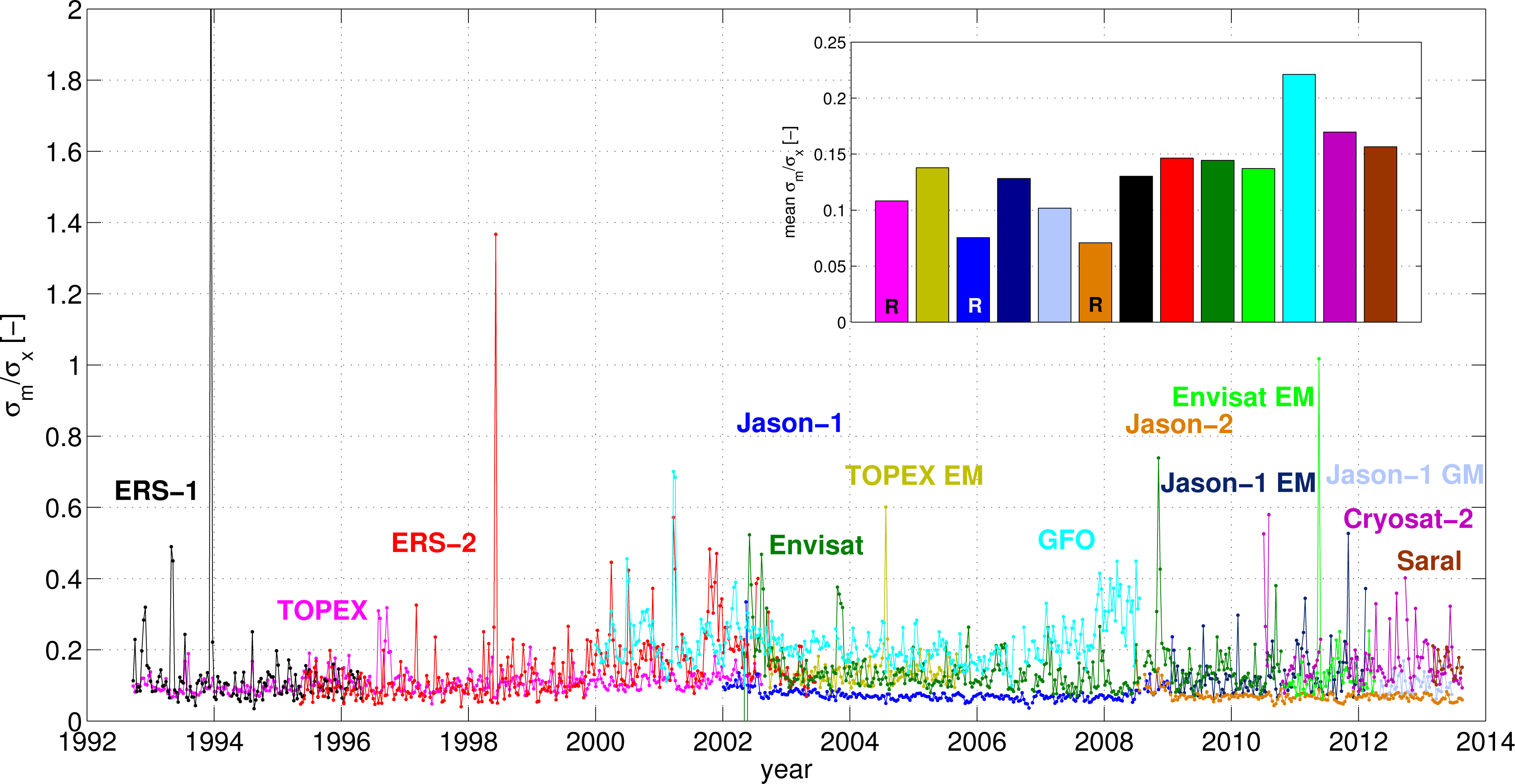
The relative weighting between the data of the different missions is achieved by means of a VCE (see Section 3.7). The estimated variance components of the different missions are plotted in
Figure 2 showing the ratio between the variance component of the individual missions,
σm, and the variance component,
σx, of crossover differences. The different accuracy levels of the missions are clearly visible:
Figure 2.
The ratio of variance components (σm/σx) for each cycle and mean variance components per mission (embedded plot, reference missions marked with “R”).
Figure 2.
The ratio of variance components (σm/σx) for each cycle and mean variance components per mission (embedded plot, reference missions marked with “R”).
GFO gets the highest variances (lowest weights), especially in the last mission phase, with missing radiometer corrections and many data gaps; Jason-2, the most accurate mission, behaves more than two times better than GFO. In principle, missions with single-frequency altimeters (inevitably relying on ionospheric model corrections) show higher variance components than those with dual-frequency sensors. The level of SARAL is relatively high as this data set lacks, at the very beginning of the mission, a consolidated SSB corrections and an optimal calibration of the radiometer. In addition to the mean level, periods with higher variance components for all missions can be identified (e.g., years 2000 to 2002, due to the higher solar activity), as well as single peaks, indicating cycles with higher values. Most of them can be accounted for by special atmospheric conditions (solar storms), missing observations or measurement problems (including orbit maneuvers), and/or problems with applied corrections.
In contrast to the variance components,
σm (
Equation (7)) and
σx (
Equation (3)), the weights of
Δ and of the pseudo observations are set manually by choosing the half weight width to be
δtx =0.3 days and
δtm =0.01 days for all missions. (see
Equations (4) and
(8)). The maximum time difference for building a crossover difference is limited to Δ
tlim =2 days, and the overlap period is set to the same value Δ
tmax =2 days. Only crossovers over ocean with SSH differences less than 1 m and standard deviations,
σΔ < 0.1 m are used. The relative influence of crossover differences and consecutive differences is defined by setting
σ0 = 0.01m (
Equation (4)).
In order to solve the rank defect, discussed in Section 3.5, one of the missions has to serve as reference mission by applying the constraint k′r = 0 to its radial errors. Due to its outstanding quality and long-term stability, TOPEX is chosen for this purpose. This implies that the mean (not the individual) radial errors for each segmentation period of 10 days (cf. Section 3.6) is forced to zero. At the end of the regular mission, TOPEX had a tandem phase with Jason-1 with both satellites flying on the same orbit with minimal time difference. Then, the TOPEX orbit was moved to an interleaved ground track. Both, tandem phase and the interleaved ground track period were used to determine the relative range offset between TOPEX and Jason-1. By a new constraint, this relative offset (0.098 m, computed from 134 cycles) is then assigned as a mean offset for Jason-1, the new reference mission. The same transfer was applied for the transition from Jason-1 to Jason-2 (applied offset to TOPEX: −0.005 m, based on 131 cycles). This way, all radial errors refer to TOPEX as reference. Note that for both transitions, the cross-calibration period between the reference mission covers more than 3.5 years.
In the following subsections, selected results of MMXO14 will be presented. The purpose is not to give a comprehensive or complete overview of all cross-calibration results for all missions. Instead, the focus will be on the most interesting results in order to demonstrate the potential and the application spectrum of the multi-mission cross-calibration approach.
4.1. Radial Errors and Its Stochastic Properties
The main result of the cross-calibration approach are time series of radial errors for all missions included in the analysis. These radial errors incorporate not only effects from the altimeter sensor (e.g., instrumental delays or drifts due to ageing effects), but also errors induced by the orbit determination process, by inaccurate geophysical corrections, or effects caused by sea state or variations of the sea level within the time period between the two crossover measurements.
The basic objective of the radial error analysis is to correct the altimeter ranges, allowing to consistently combine the data of all missions and deriving multi-mission products. The merging of altimeter data from different missions not only improves the spatio-temporal resolution, but also helps to construct time series, extending the lifetime of a single mission. In addition, the time series can be used to derive stochastic characterizations of the different missions by auto-covariance functions and power spectra (see Section 3.8). Moreover, the radial errors are the basis for further derivation of post-processing products, such as mean range biases or geographically correlated errors.
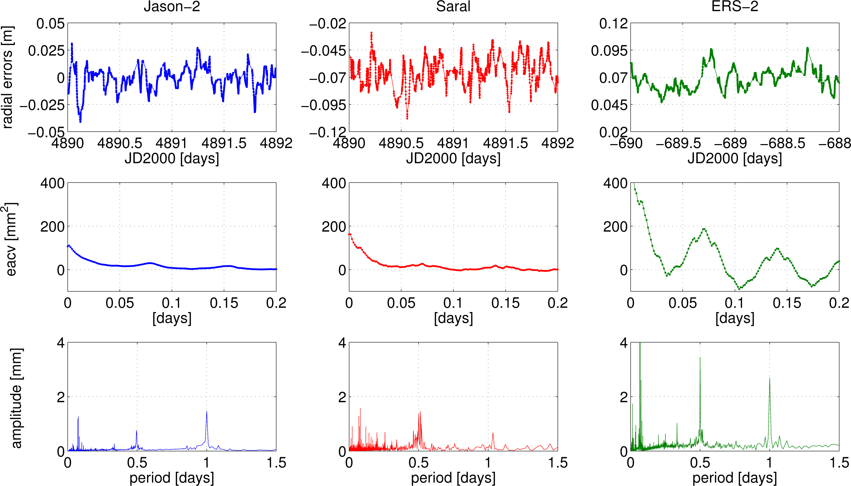
The first row in
Figure 3 shows two-day subsets of radial errors estimated for Jason-2, SARAL, and ERS-2. Note, the scaling of the radial errors is equal, but the range has been adapted to the different range biases. The second row of
Figure 3 displays empirical auto-covariance functions
Crr,
cf.
Equation (22), derived with the complete time series of radial errors. From these plots the variances of the radial errors for the three missions can be deduced (Jason-2: 1.0 cm; SARAL: 1.3 cm; ERS-2: 2.0 cm). Moreover, the temporal correlations within the time series are visible. In all three plots, relative maxima can be seen after one (two or more) orbital revolutions. This 1/rev -effects is particular outstanding for ERS-2, and it is much stronger than for the other two missions. This is also visible in the power spectra shown in the last row of
Figure 3. Again, a common scaling has been applied to the spectra plots in order to make them comparable. ERS-2 obeys a maximum amplitude of more than 10 mm (above the displayed amplitude range) for a period of about 0.07 days (which corresponds to just one revolution). Smaller amplitudes are present at periods of 0.5 and one day. In contrast to that, Jason-2 and SARAL amplitudes remain below 2 mm. For Jason-2, the most prominent period is at one day with 1.5 mm amplitude. For SARAL, the maximum amplitude of 1.6 mm appears at a period of 0.08 days; outside the displayed range there is another period of about 8.3 days with an amplitude of about 1.3 mm. Probably, most of these frequencies result from inaccurate orbit determination.
4.2. Global Mean Range Biases between the Missions
Range biases for each mission are computed for every 10-day period. For most of the missions, the time series of range biases over the whole mission lifetime shows little scatter and no systematic effects. Thus, the computation of one global mean range bias seems acceptable. These global mean range biases have been compiled in
Table 3 [
47–
49] The estimated global mean range biases agree quite well to the absolute values derived at the
in-situ calibration sites. The most recent results were presented at the OSTST (Ocean Surface Toprography Science Team) meeting in Boulder, 2013, and are also summerized in
Table 3. For the Corsica calibration site, absolute biases for 8 different missions were provided. Most of the values agree to within a few millimeter to the results derived from MMXO14. Only for some missions, larger discrepancies can be seen, namely for Jason-1 (difference of 2 cm) and ERS-2 (difference of 13 cm with values of opposite sign!). For Jason-1, the MMXO14 result perfectly agrees to the Harvest estimate of 96 mm (with GDR-D orbit), but for ERS-2, unfortunately, no other calibration site provides any bias. Thus, this discrepancy cannot be explained.
Analyzing the time series of range bias clearly reveals systematic effects for some missions (we show only the most outstanding results of MMXO14). The ENVISAT mission, for example, exhibits a significant offset of about 3 cm between the range biases of Side A and Side B. This happens mid-2006, when the measurements were temporarily taken from the redundant system. For ICESat, operating only in short episodic laser periods, the estimated range biases of individual periods vary significantly. This explains the large standard deviation in
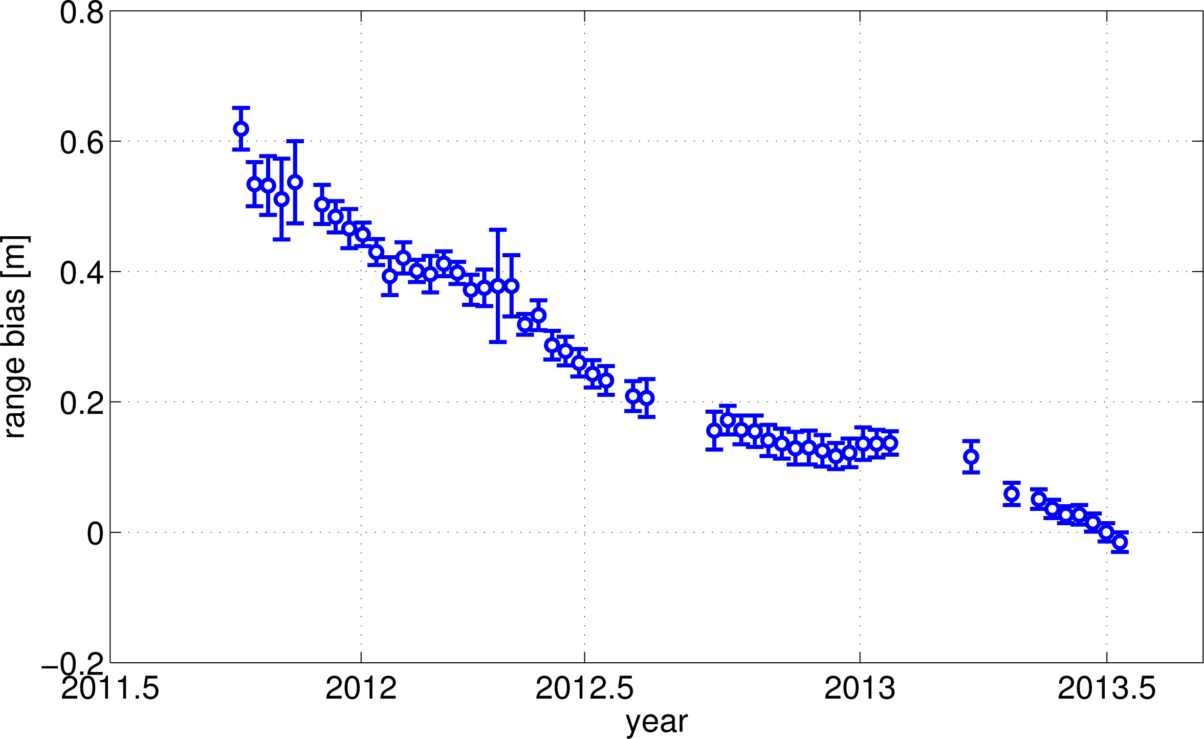
Table 3, due not only to random effects, but also systematic differences. The range biases for HY-2A IGDR data shows a significant negative trend of about
−0.3 m/year,
cf.
Figure 4. The standard deviation given in
Table 3 also reflects these systematic effects.
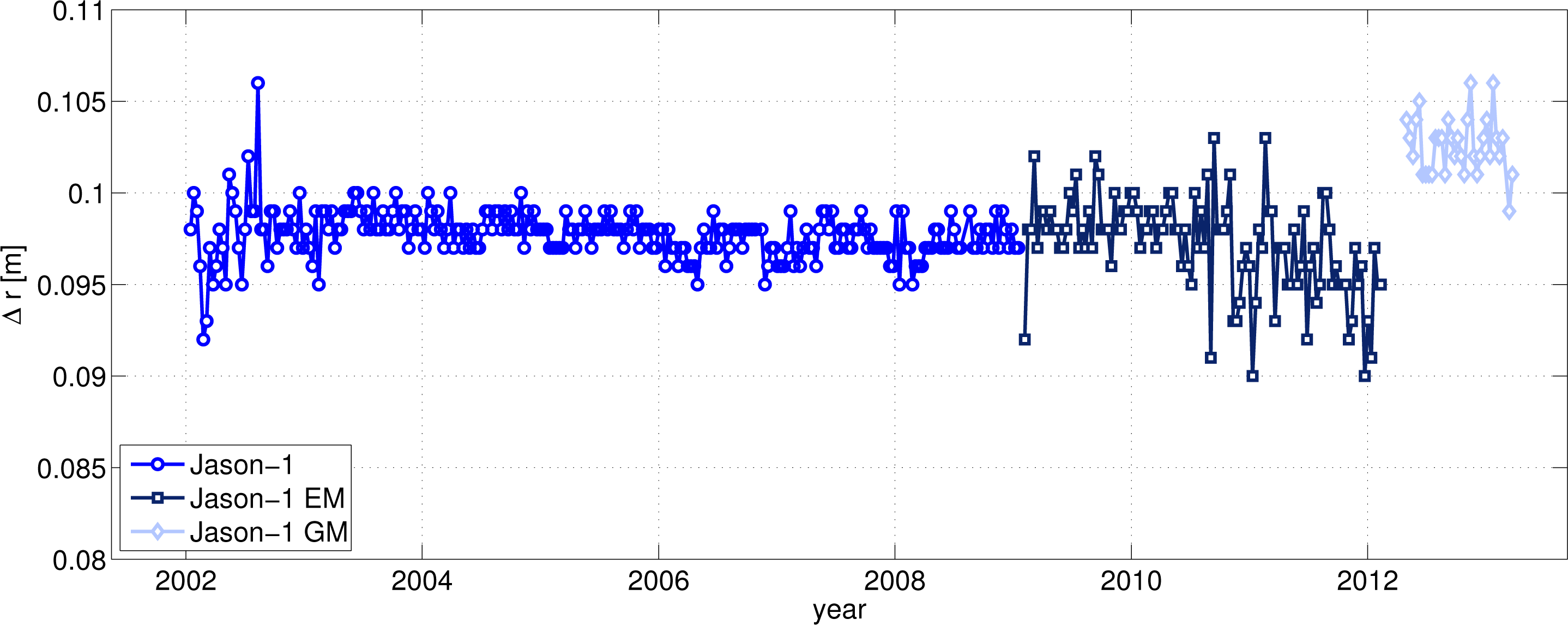
Typically, the range bias does not change in case of an orbit event,
i.e., between the core mission and the extended mission on an interleaved ground track. However, for Jason-1, a significant offset of about 6 mm between the range bias of the geodetic mission phase and the two earlier mission phases occur, as can be seen in
Figure 5. The source of this offset is still under investigation. It might be related to the new orbit height, to some modifications within the Level 2 processing chain (change in the pulse repetition frequency) or jumps in the wet tropospheric correction from the radiometer.
The different noise levels of the Jason-1 range biases is due to the change of the reference mission (see Section 3.6). Between TOPEX cycle 366 and 603 (August 2002 to January 2009), Jason-1 serves as reference mission, causing a much smoother time series. After the end of the primary Jason-1 mission, Jason-2 is used as reference.
The last part of the Jason-1 EM range biases seems to include a moderate negative trend, which is not significant, due to the relative high scatter of the data within this time period. The source of both effects (higher scatter after cycle 655 and possible drift) is not yet understood. Unfortunately, the time series can not be extended to allow for a further inspection.
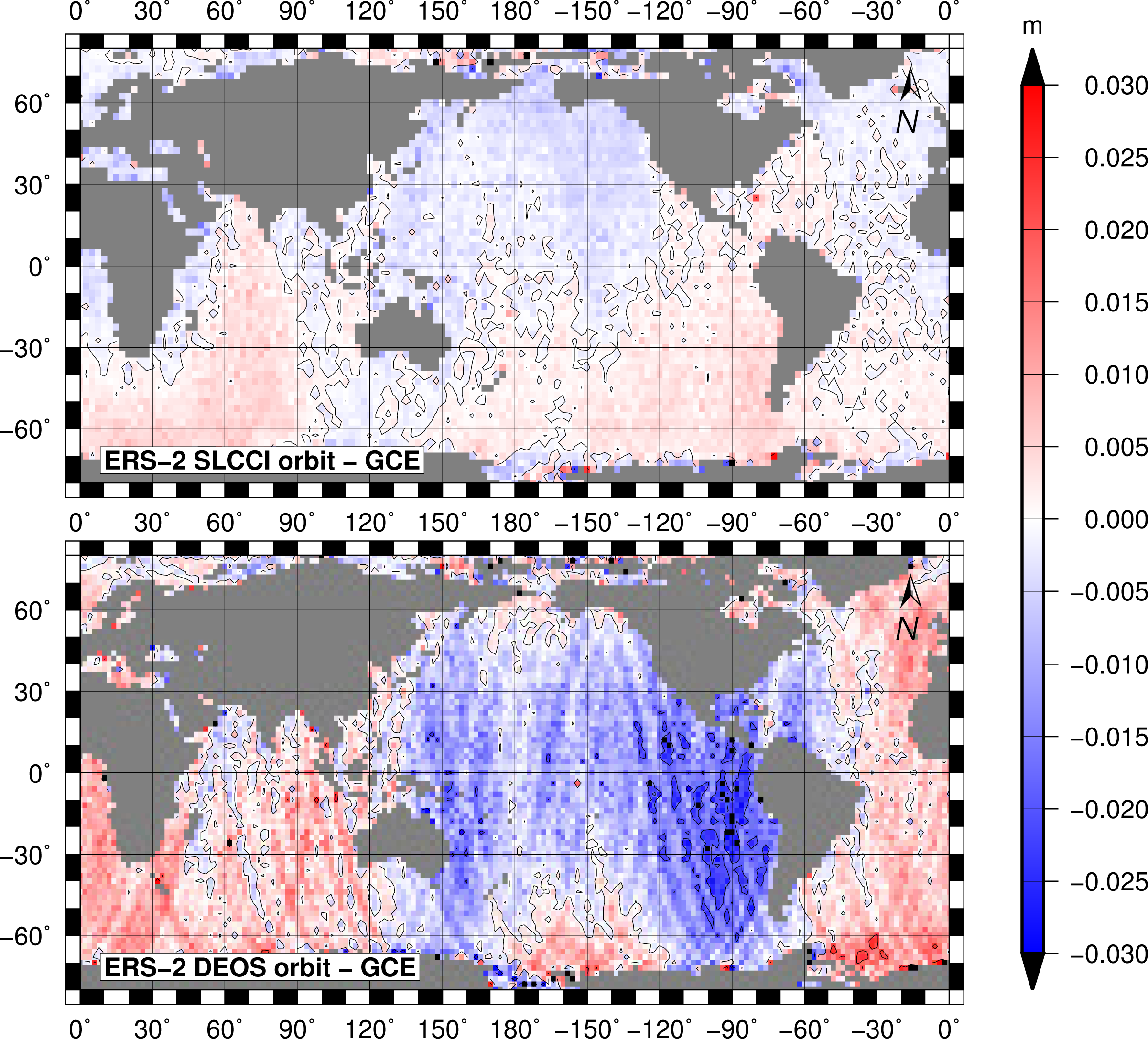
4.4. Geo-Centre Realization of Altimeter Satellite Orbits
Some dedicated pattern in GCE can already indicate systematic shifts of the centre-of-origin realization of the satellite orbits. For example, a clear north-south tilt in GCE illustrates a shift in the z-component, Δz. However, since the GCE are computed over the whole mission lifetimes, no temporal variations or drifts are visible. For investigations aiming on monitoring geo-centre variations, the derivation and analysis of centre-of-origin shifts from radial errors (as described in Section 3.8) is meaningful.
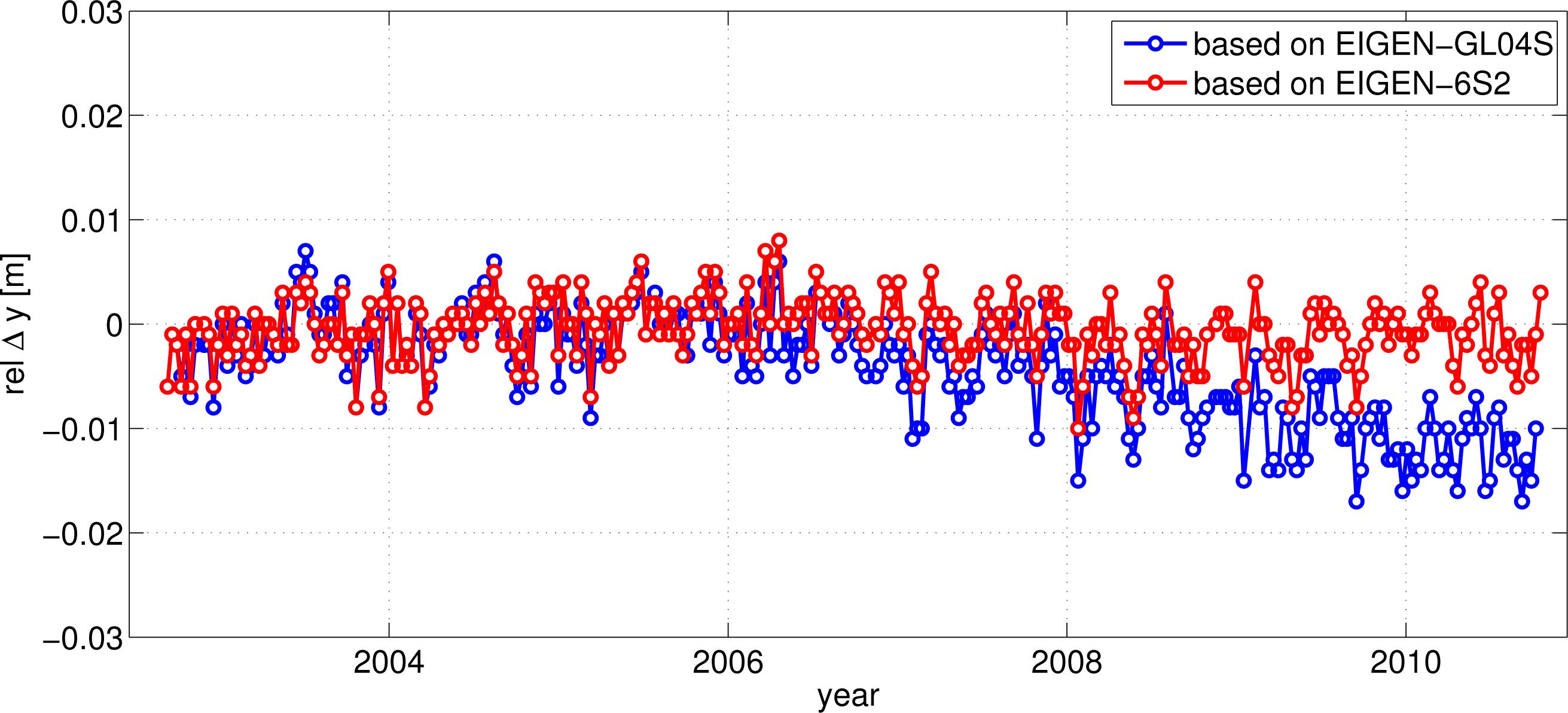
For recent altimeter data sets and recent orbit solutions most of the centre-of-origin shift does not differ significantly from zero. However, some effects of the shift become visible if the gravity field models used for precise orbit determination do not properly account for temporal variations of gravity. This effect is mainly reflected in the
y-component of the origin shifts.
Figure 7 shows the relative differences of the
y-shift between Jason-1 and ENVISAT using most recent orbits (SLCCI VER6, based on the EIGEN-6S2 gravity field, a modification of EIGEN-6S [
51], in red) and older ones (SLCCI VER2, based on the EIGEN-GL04S [
52] gravity field, in blue). More details on orbits based on time-variable gravity can be found in [
33].
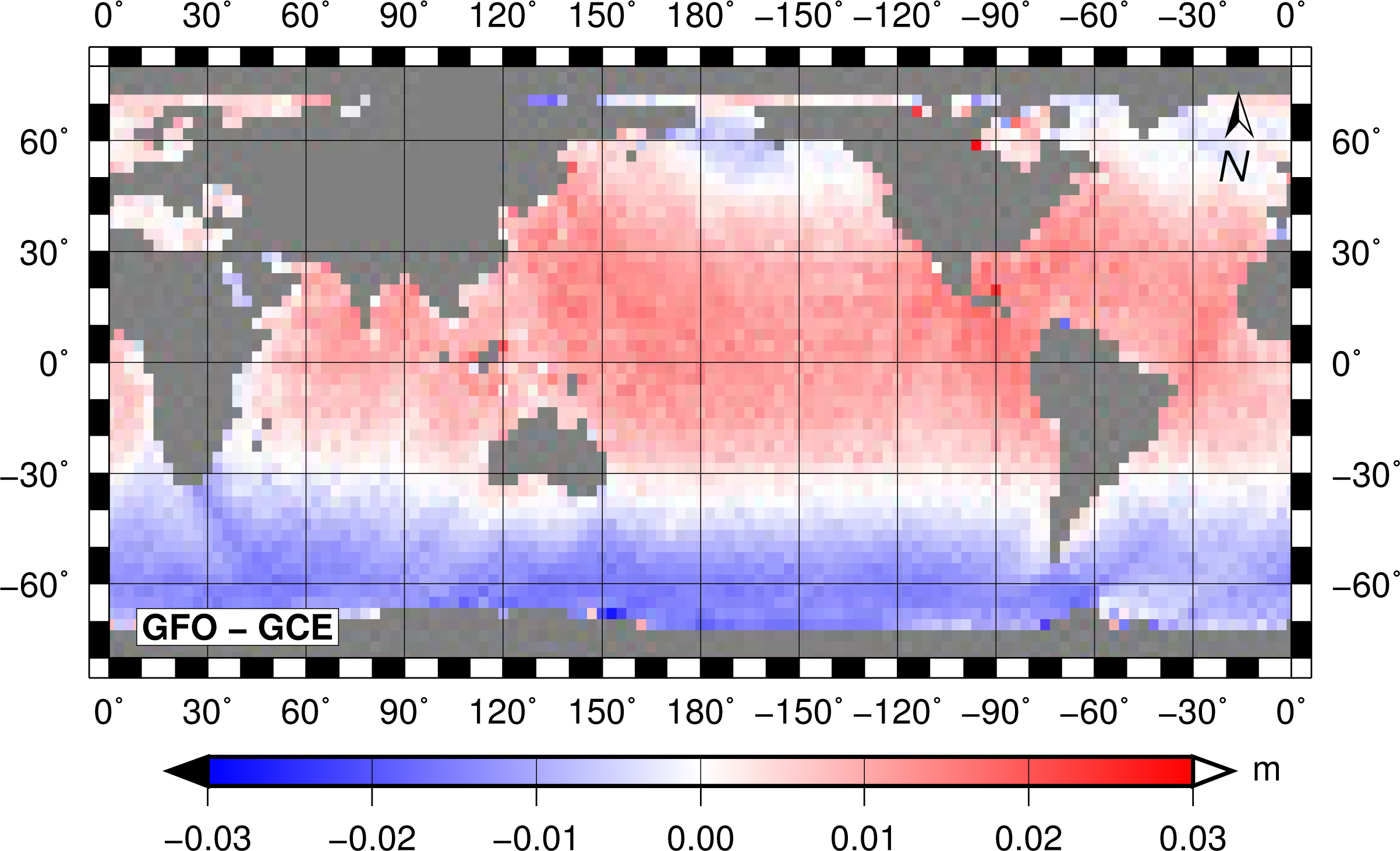
For most missions the degree 2 coefficients of the spherical harmonic series (
Equation (24)) are not significant, with one exception: GFO. The orbit of this satellite is difficult to model, as the mission has neither DORIS nor GPS observations available. Thus, the most recent orbit for this mission (GSFC std0905) uses satellite laser ranging, Doppler data and altimeter crossover data to estimate the orbit with an accuracy of 3–4 cm in the radial component [
53]. The orbit errors directly map in the radial and the geographically correlated errors and are also reflected in the center-of-origin realization. The estimated spherical harmonic coefficients for GFO are listed in
Table 4. Whereas the orientation of the rotation axis (
C21 and
S21) do not differ significantly from the TOPEX realization, the
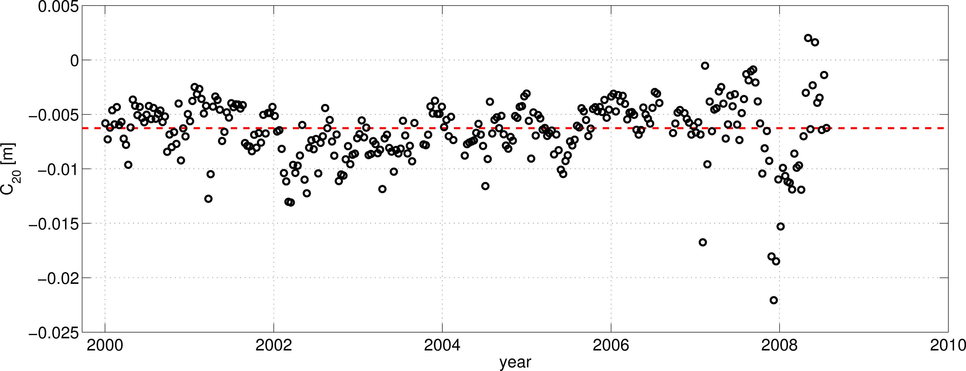
C20 term (corresponding to the flattening) shows a clear offset of 6.5 mm, yielding to a latitude dependent pattern in GCE (see
Figure 8). The temporal evolution of the
C20-term is plotted in
Figure 9. The reason for this effect is still under investigation. It might be related to inconsistent handling of permanent and/or long-period tides. However, the std0905 orbit is already a significant improvement over the originally GDR-B orbit, which has additional significant offsets to TOPEX in
C11 and
S11.
5. Conclusions
The multi-mission cross-calibration of satellite altimeters is a powerful analysis tool to derive consistent multi-mission data, allowing one to merge data from different missions in order to improve the space-time sampling of sea surface heights and to construct a long-term data record (extending the lifetime of single missions) for global and regional sea level change studies. The modelling of radial errors is based on a rather simple concept, the discrete crossover analysis adjusting both crossover and consecutive differences. The system has to be regularized by a single constraint applied to a reference mission. In a multi-mission scenario, the normal equation becomes rather huge, but remains sparse and can be solved iteratively by a conjugate gradient algorithm. A variance component estimate ensures an objective relative weighting of missions with different precision. The redundancy of the adjustment grows with the number of missions, operating simultaneously. Already, with two contemporaneous missions, the strength of the analysis is sufficient to obtain a robust estimate of the radial errors. Once the time series of radial errors has been estimated, a post processing allows to characterize their stochastic properties by auto-covariance functions and to identify systematic error pattern in terms of centre-of-origin shifts or geographically correlated errors.
The present cross-calibration approach has been applied many times and is going to be updated whenever the data holdings have been extended, improved by new data releases, better correction models or reprocessed orbits. The selected results shown in the present paper demonstrate that robust relative range biases are obtained for the full lifetime of (nearly all) altimeter systems with completely different orbit configuration and sampling characteristics. The error analysis is able to identify systematic errors, alteration in the processing chain and inconsistent geocentring of the orbits. The present analysis also identified data problems of rather new missions (as HY-2A), but also weaknesses and unresolved issues of past missions (such as GFO or Jason-1).
A final remark to the GCE pattern and other systematic effects: In general, an improved orbit solution is taken to identfy the GCE pattern of the previous orbit solution by just comparing, in retrospect, new and old orbits. Based on the strong redundancy, achieved by computing crossover differences in all combinations between contemporaneous altimeter missions, the present approach is able to estimate GCE pattern directly for the most recent orbital ephemeris. This reveals the potential of the present approach for calibration and verification for satellite altimeter missions.


