Spatio-Temporal Assessment of Tuz Gölü, Turkey as a Potential Radiometric Vicarious Calibration Site


Abstract
:1. Introduction
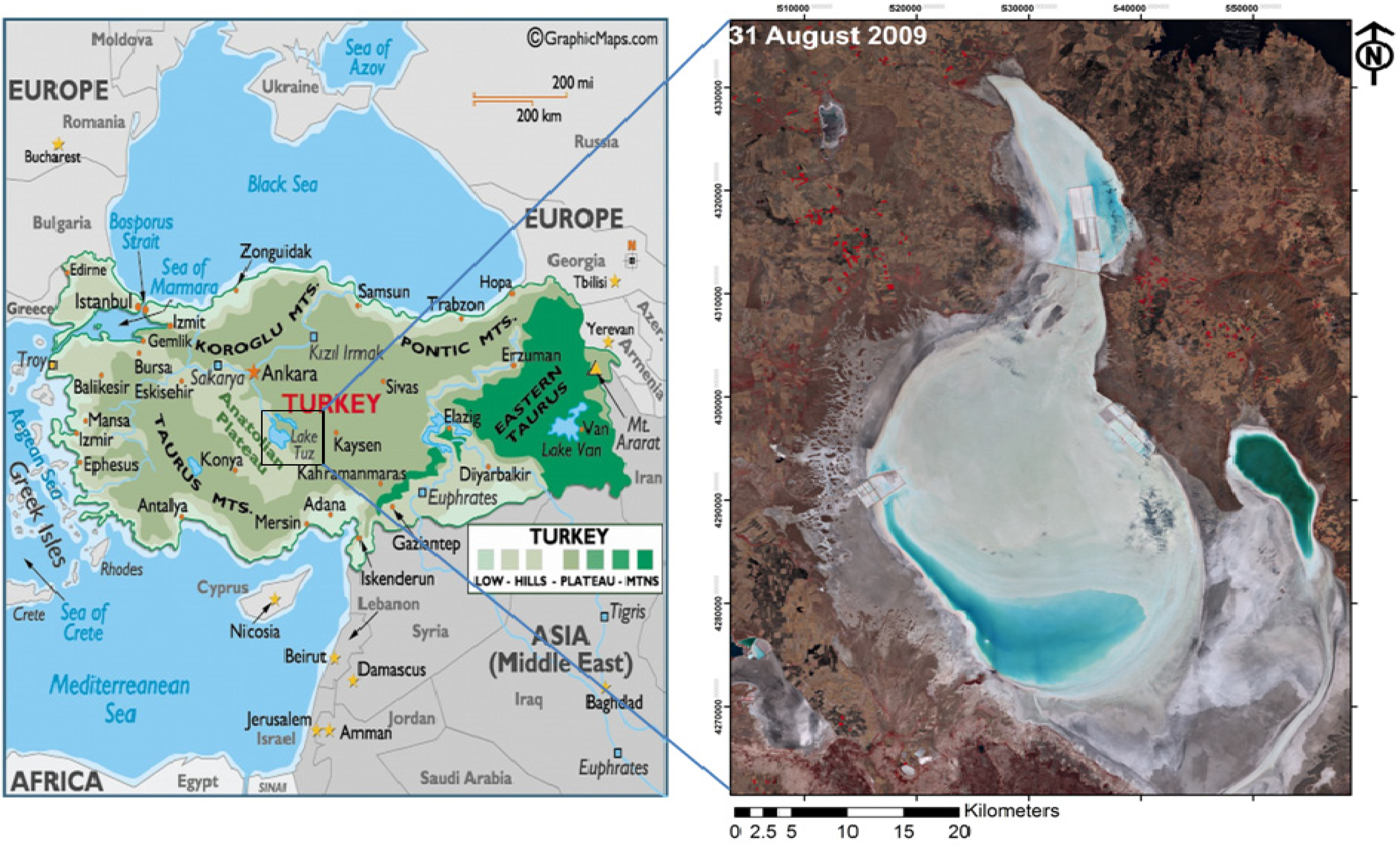
2. Site Description
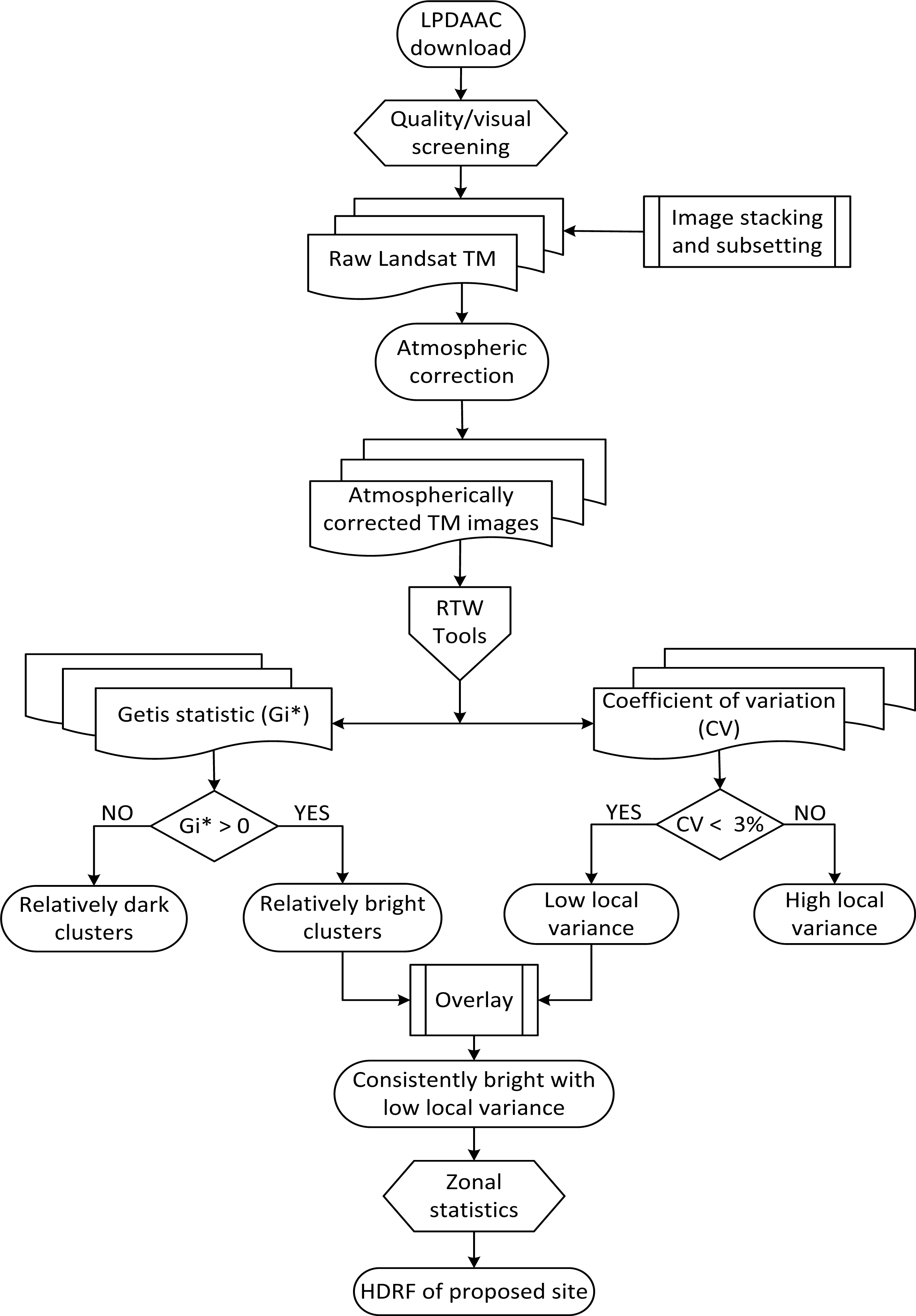
3. Method
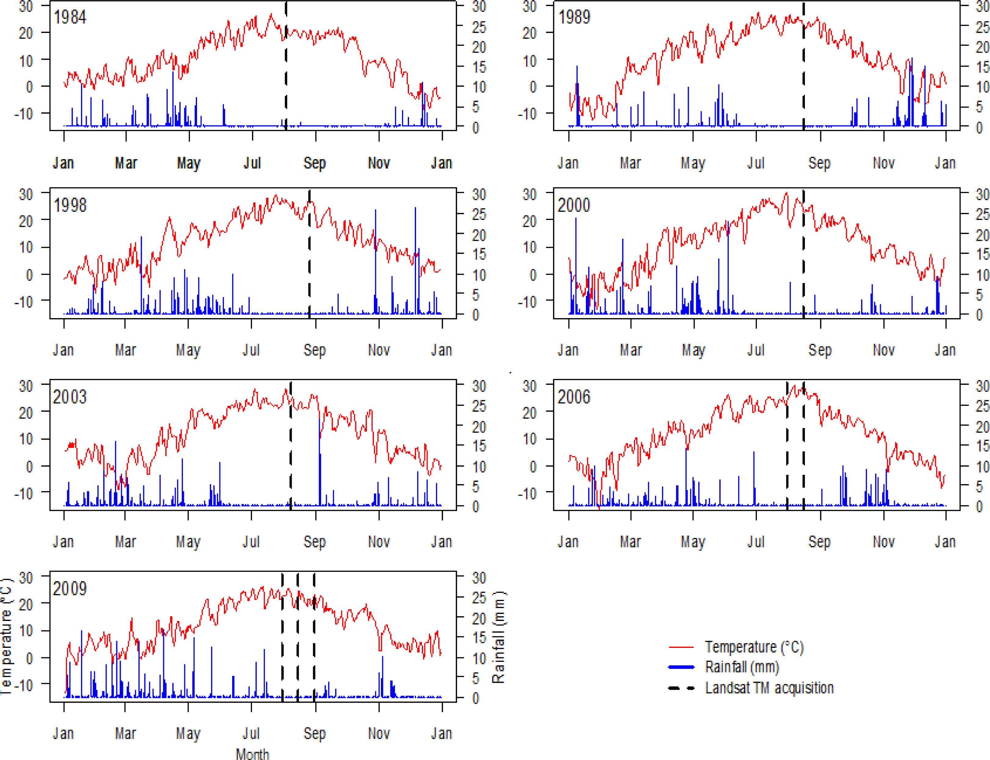
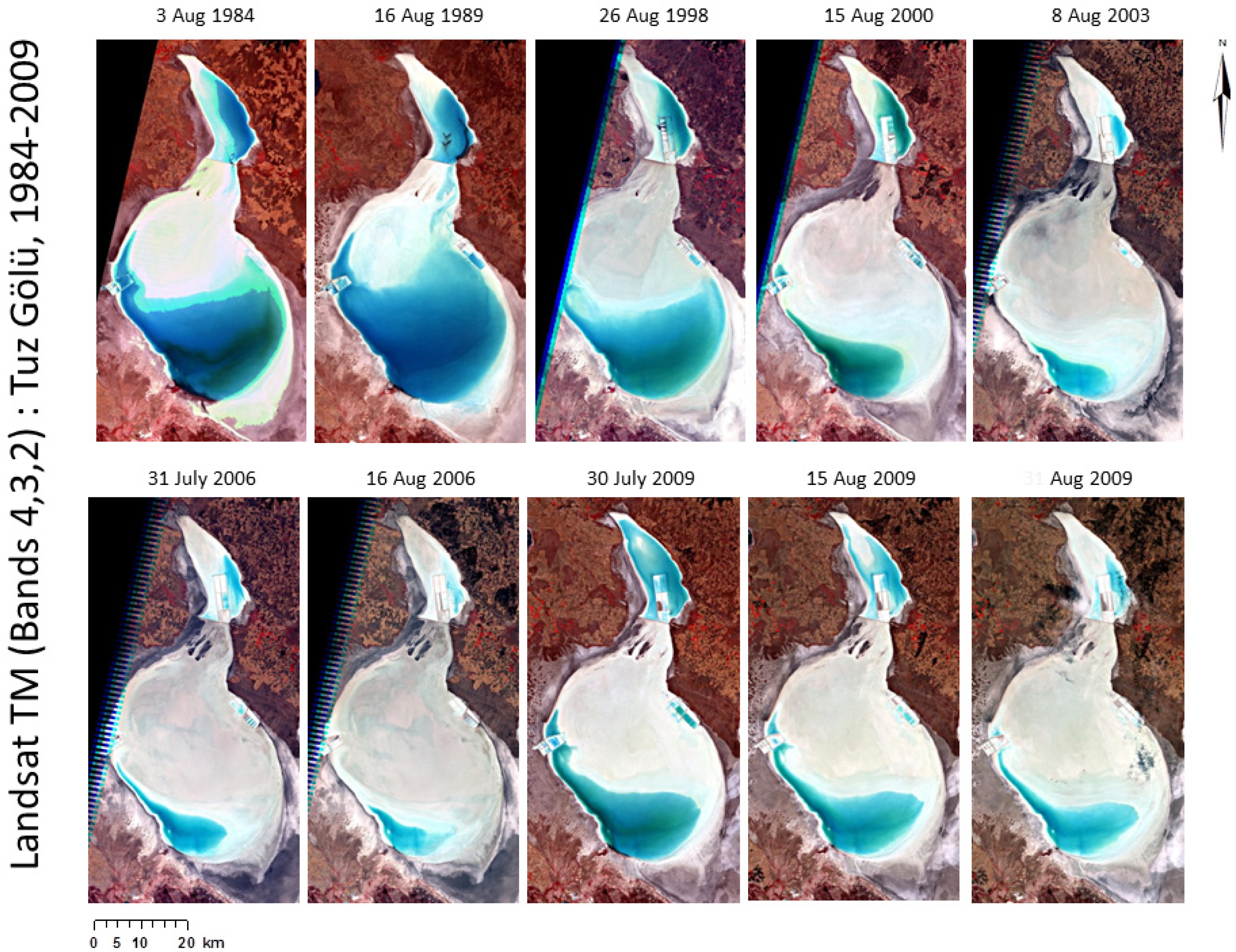
3.1. Data Acquisition and Processing
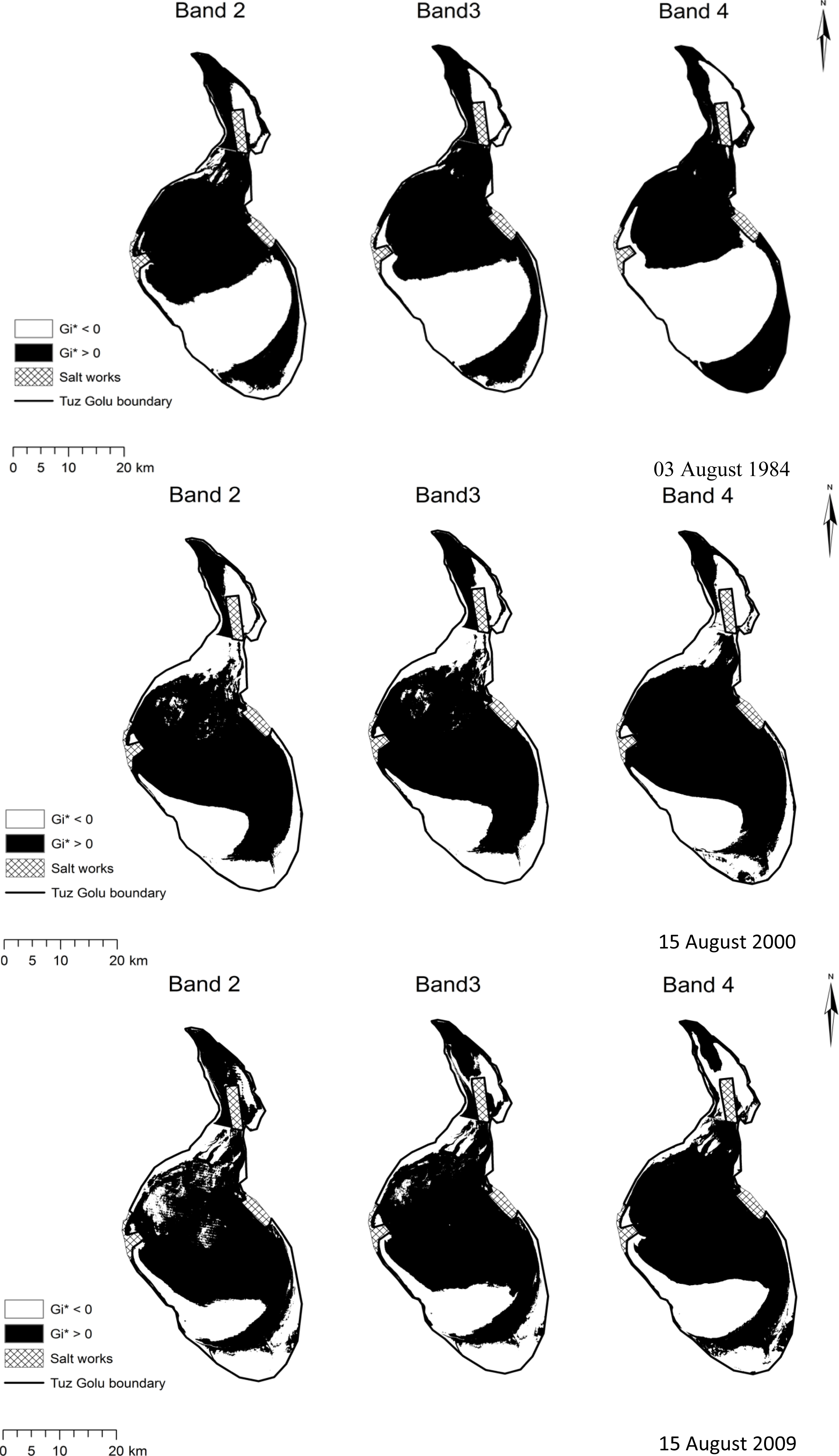
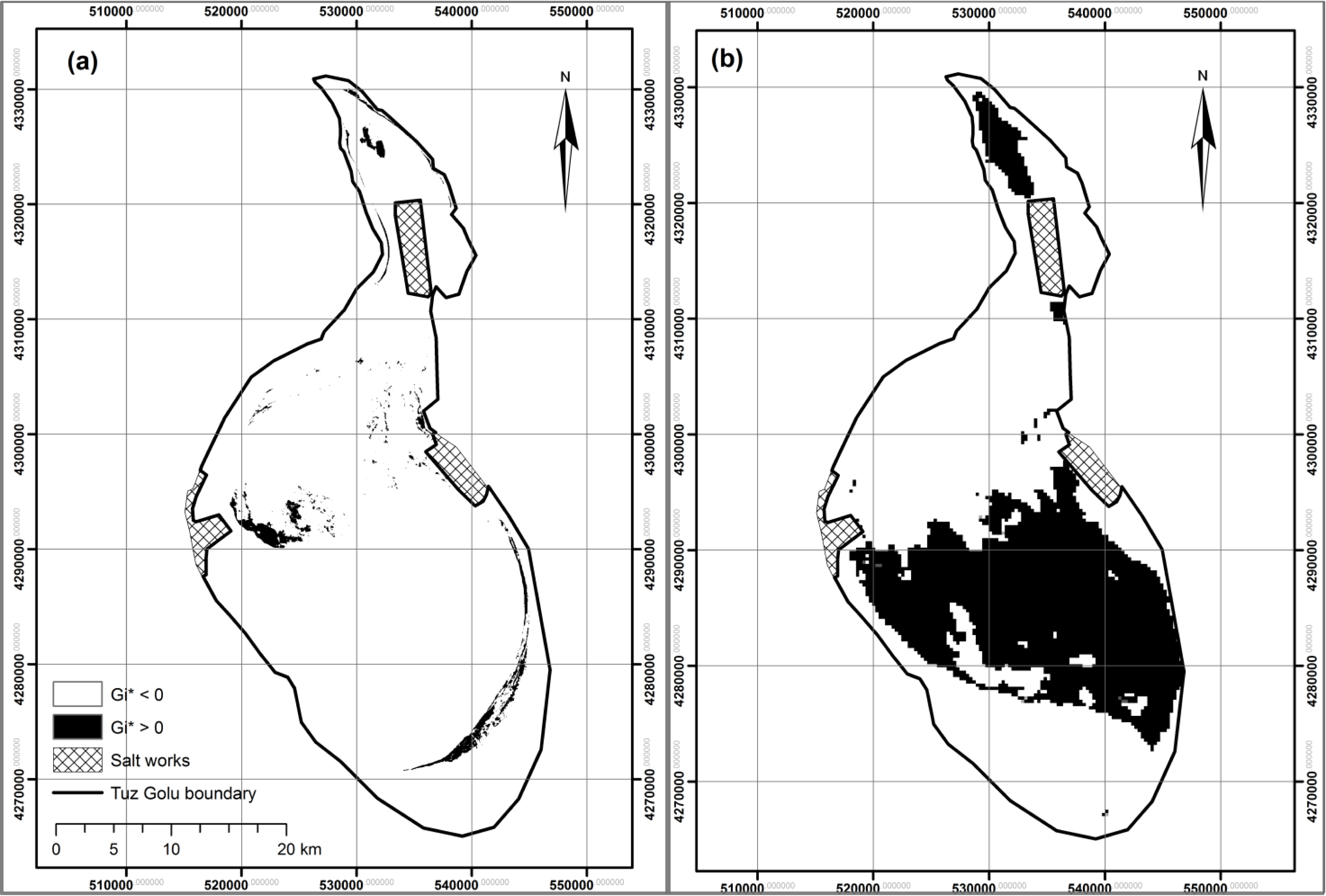
3.2. Analysis of Clustering (Gi*)
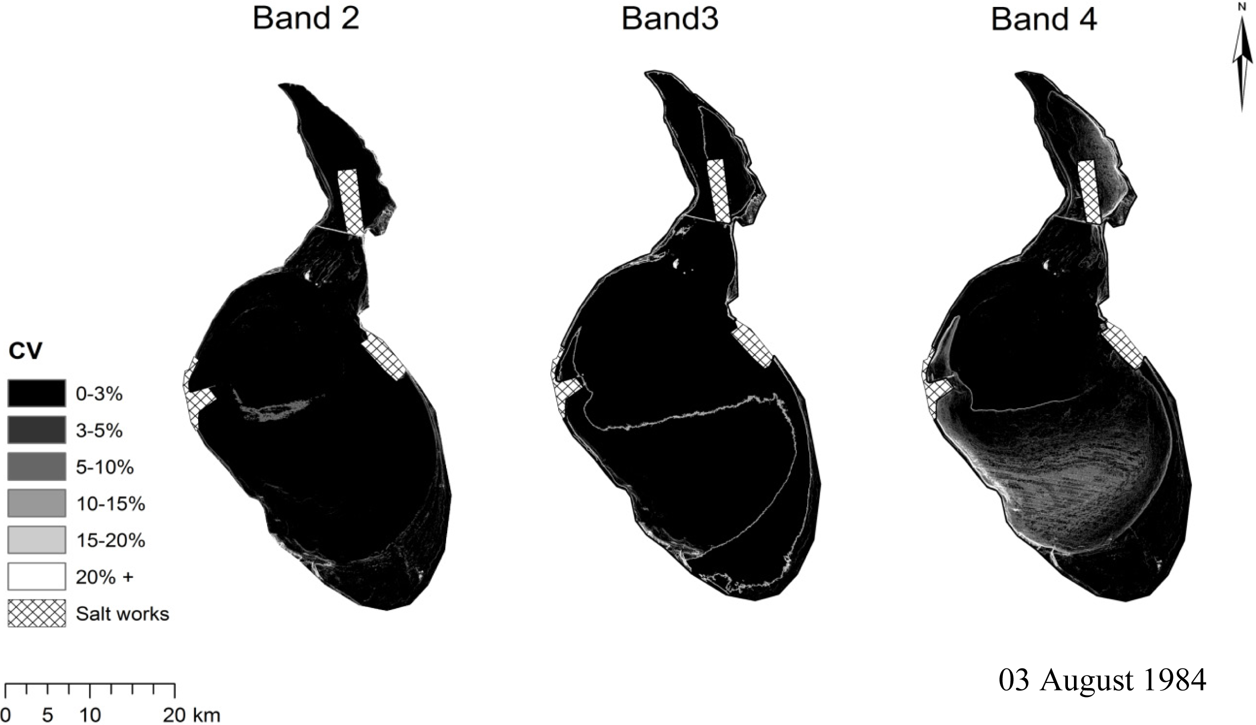
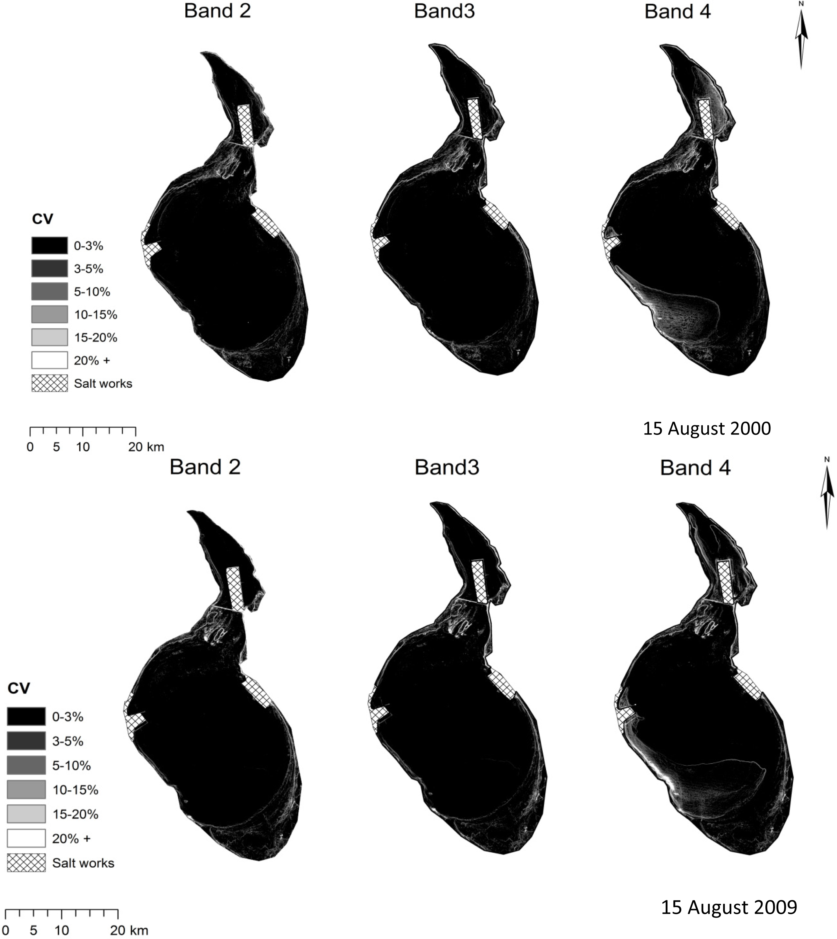
3.3. Analysis of Local Variability (CV)
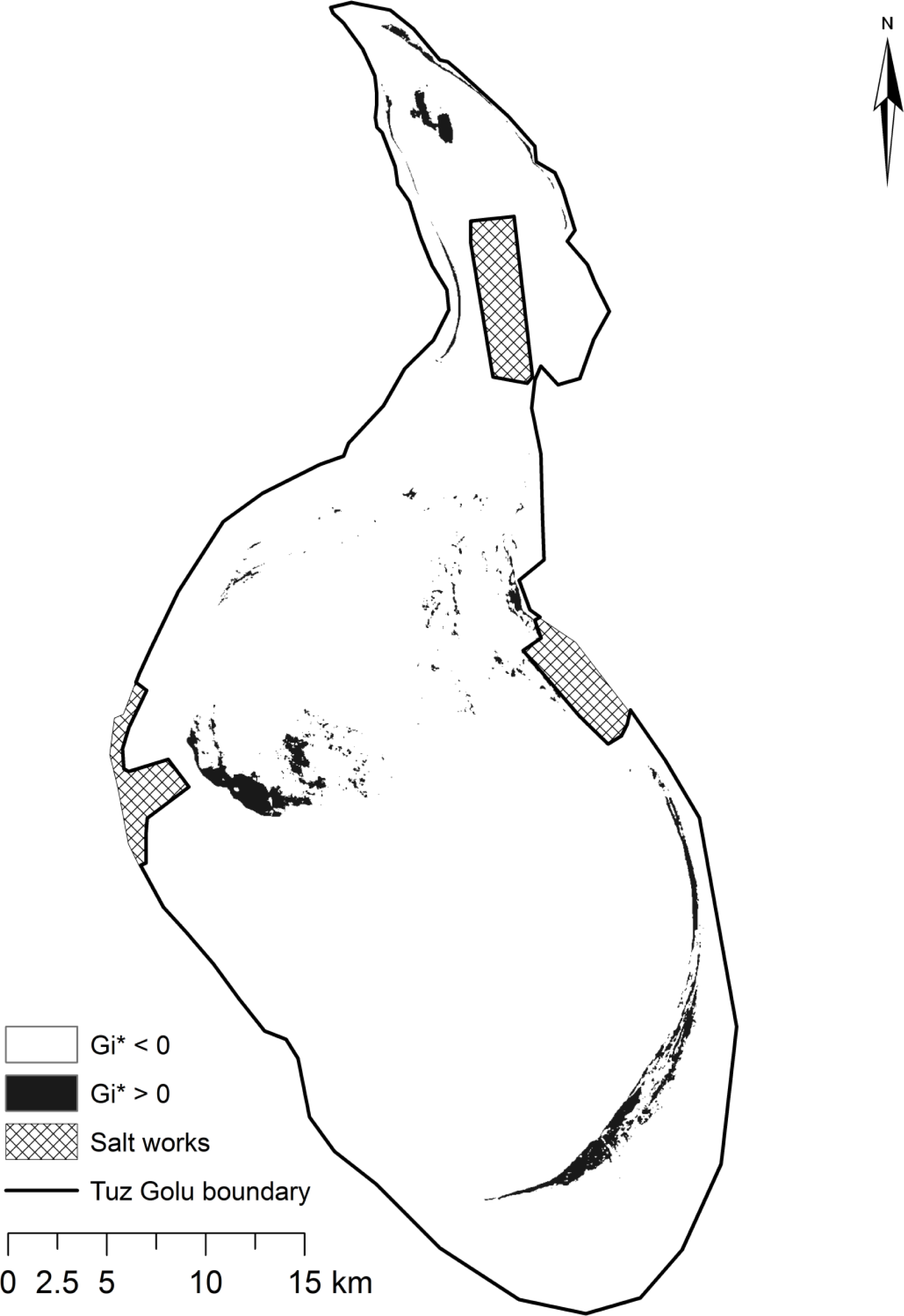
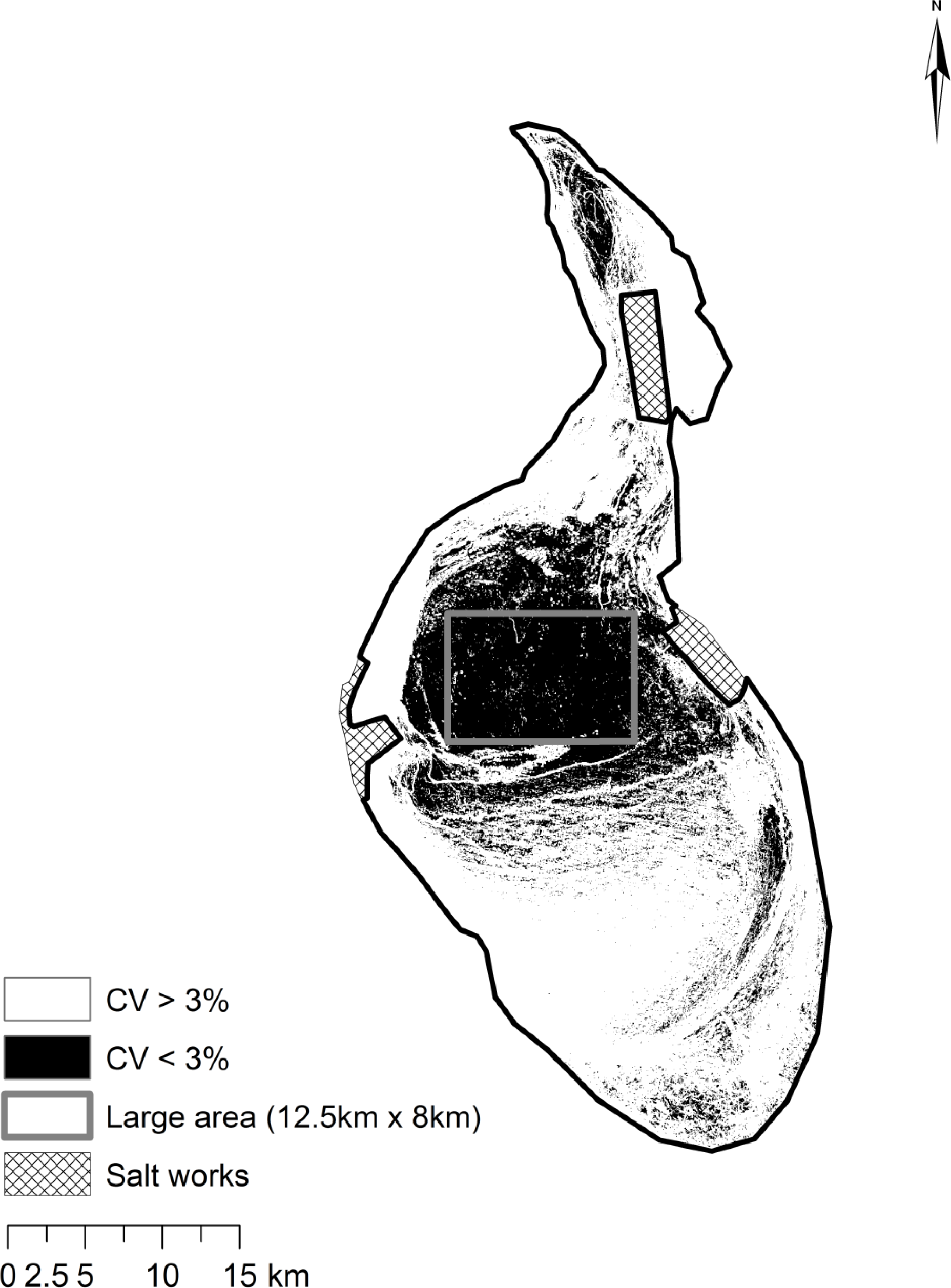
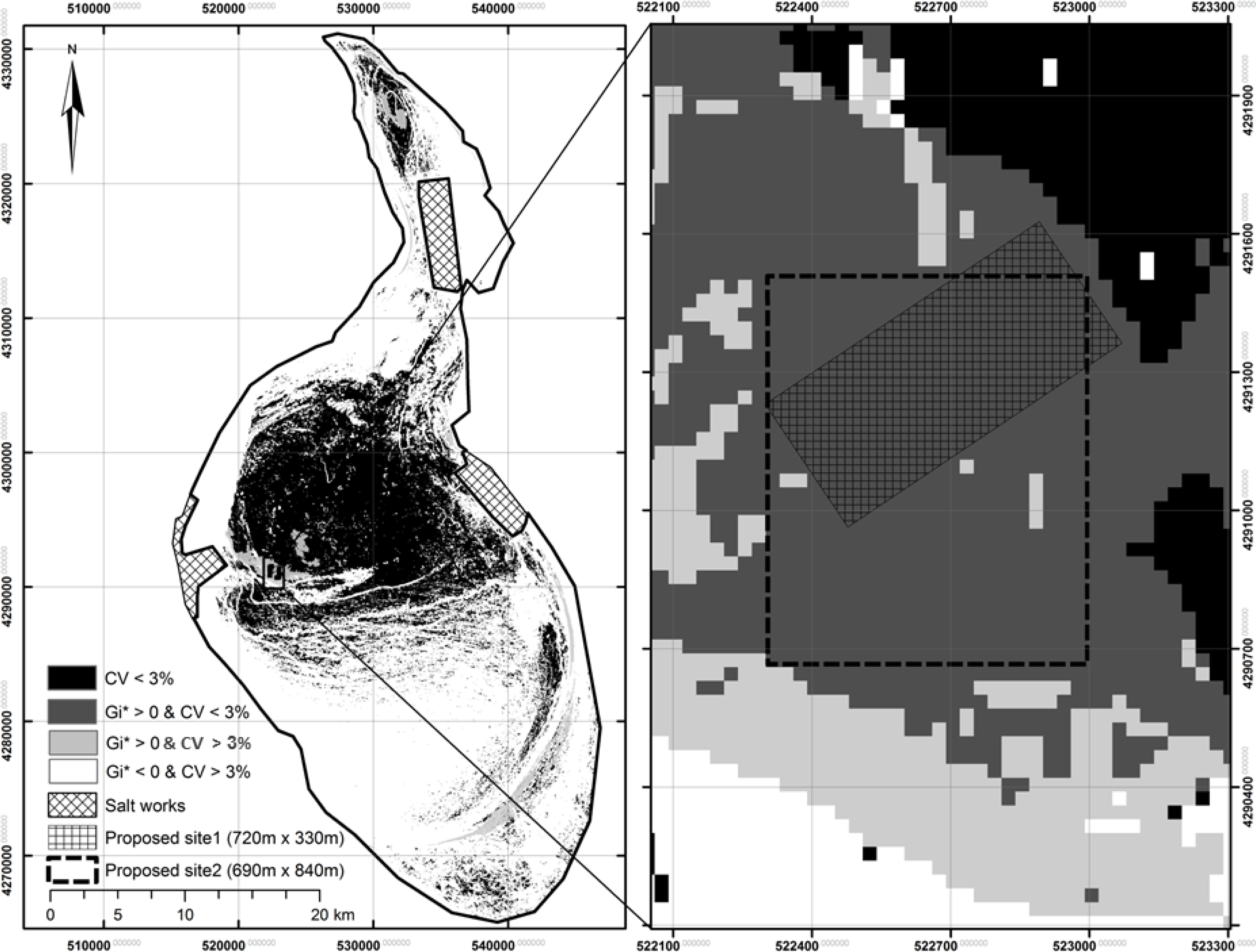
3.4. Identifying Spatially Homogeneous Areas
- Criterion 1: Gi* > 0;
- Criterion 2: CV < 3%;
- Criterion 3: HDRF > 30%;
- Criterion 4: Persistence of criteria 1–3 over time.
4. Results
4.1. Spatial Clustering
4.2. Local Variability
4.3. Spatial Homogeneity
4.4. HDRF of Proposed Site
5. Discussion
6. Conclusion
Supplementary Information
remotesensing-06-02494-s001.pdfAcknowledgments
Author Contributions
Conflicts of Interest
References
- Bannari, A.; Omari, K.; Teillet, P.M.; Fedosejevs, G. Potential of Getis statistics to characterize the radiometric uniformity and stability of test sites used for the calibration of Earth observation sensors. IEEE Trans. Geosci. Remote Sens 2005, 43, 2918–2925. [Google Scholar]
- Fox, N.P. Validated Data Removal of Bias through Traceability to SI Units. In Post-Launch Calibration of Satellite Sensors; Morain, S.A., Budge, A.M., Eds.; Taylor and Francis: London, UK, 2004. [Google Scholar]
- Teillet, P.M.; Horler, D.N.H.; O’Neill, N.T. Calibration, validation, and quality assurance in remote sensing: A new paradigm. Can. J. Remote Sens 1997, 23, 401–414. [Google Scholar]
- Gürol, S.; Behnert, I.; Özen, H.; Deadman, A.; Fox, N.; Leloğlu, U.M. Tuz Gölü: New CEOS reference standard test site for infrared visible optical sensors. Can. J. Remote Sens 2010, 36, 553–565. [Google Scholar]
- Leloğlu, U.M.; Gürbüz, H.; Őzen, H.; Gürol, S. Characterization of the Spatial Uniformity of the Tuz Gölü Calibration Test Site. Proceedings of ISPRS Workshop on Modeling of Optical Airborne and Spaceborne Sensors, Istanbul, Turkey, 11–13 October 2010.
- Kneubühler, M.; Schaepman, M.E.; Thome, K. Long-Term Vicarious Calibration Efforts of MERIS at Railroad Valley playa (Nevada)–An update. Proceedings of the Second Working Meeting on MERIS and AATSR Calibration and Geophysical Validation (MAVT-2006), Frascati, Italy, 20–24 March 2006.
- Teillet, P.M.; Barsi, J.A.; Chander, G.; Thome, K.J. Prime candidate Earth targets for the post-launch radiometric calibration of space-based optical imaging instruments. Proc. SPIE 2007. [Google Scholar] [CrossRef]
- Thome, K.J. Absolute radiometric calibration of Landsat 7 ETM+ using the reflectance-based method. Remote Sens. Environ 2001, 78, 27–38. [Google Scholar]
- Schaepman-Strub, G.; Schaepman, M.E.; Painter, T.H.; Dangel, S.; Martonchik, J.V. Reflectance quantities in optical remote sensing—Definitions and case studies. Remote Sens. Environ 2006, 103, 27–42. [Google Scholar]
- Milton, E.J.; Schaepman, M.E.; Anderson, K.; Kneubühler, M.; Fox, N. Progress in field spectroscopy. Remote Sens. Environ 2009, 113(S1), S92–S109. [Google Scholar]
- de Vries, C.; Danaher, T.; Denham, R.; Scarth, P.; Phinn, S. An operational radiometric calibration procedure for the Landsat sensors based on pseudo-invariant target sites. Remote Sens. Environ 2007, 107, 414–429. [Google Scholar]
- Woodcock, C.E.; Strahler, A.H. The factor of scale in remote sensing. Remote Sens. Environ 1987, 21, 311–332. [Google Scholar]
- Rondeaux, G.; Steven, M.D.; Clark, J.A.; Mackay, G. La Crau: A European test site for remote sensing validation. Int. J. Remote Sens 1998, 19, 2775–2788. [Google Scholar]
- Scott, K.P.; Thome, K.J.; Brownlee, M.R. Evaluation of Railroad Valley playa for use in vicarious calibration. Proc. SPIE 1996. [Google Scholar] [CrossRef]
- Bannari, A.; Omari, K.; Teillet, P.M.; Fedosejevs, G. Multi-sensor and multi-scale survey and characterization for radiometric spatial uniformity and temporal stability of Railroad Valley playa (Nevada) test site used for optical sensor calibration. Proc. SPIE 2004. [Google Scholar] [CrossRef]
- Gurol, S.; Ozen, H.; Leloglu, U.M.; Tunali, E. Tuz Gölü: New absolute radiometric calibration test site. Int. Arch. Photogramm. Remote Sens. Spat. Inf. Sci 2008, 37, 35–39. Available Online: http://www.isprs.org/proceedings/XXXVII/congress/1_pdf/06.pdf (accessed on 12 March 2014). [Google Scholar]
- Getis, A.; Ord, J.K. The analysis of spatial association by use of distance statistics. Geogr. Anal 1992, 24, 189–206. [Google Scholar]
- Getis, A. Spatial Dependence and Heterogeneity and Proximal Databases. In Spatial Analysis and GIS; Taylor and Francis: London, UK, 1994; pp. 105–120. [Google Scholar]
- Ord, J.K.; Getis, A. Local spatial autocorrelation statistics: Distributional issues and an application. Geogr. Anal 1995, 27, 286–306. [Google Scholar]
- Gokmen, M.; Vekerdy, Z.; Lubczynski, M.W.; Timmermans, J.; Batelaan, O.; Verhoef, W. Assessing groundwater storage changes using remote sensing-based evapotranspiration and precipitation at a large semiarid basin scale. J. Hydrometeorol 2013, 14, 1733–1753. [Google Scholar]
- Camur, M.Z.; Mutlu, H. Major-ion geochemistry and mineralogy of the salt lake (Tuz Gölü) basin, Turkey. Chem. Geol 1996, 127, 313–329. [Google Scholar]
- Kilic, O.; Kilic, A.M. Salt crust mineralogy and geochemical evolution of the salt lake (Tuz Gölü), turkey. Sci. Res. Essays 2010, 5, 1317–1324. [Google Scholar]
- Helder, D.L.; Markham, B.L.; Thome, K.J.; Barsi, J.A.; Chander, G.; Malla, R. Updated radiometric calibration for the Landsat-5 thematic mapper reflective bands. IEEE Trans. Geosci. Remote Sens 2008, 46, 3309–3325. [Google Scholar]
- Richter, R. Atmospheric/Topographic Correction for Satellite Imagery—ATCOR-2/3 User Guide; Version 6.3; Remote Sensing Data Centre Publication DLR-IB 565-01/07; German Aerospace Centre: Wessling, Germany, 2007. [Google Scholar]
- Wilson, R.T. RTWTools. 2011. Available online: http://www.rtwtools.rtwilson.com/ (accessed on 14 March 2014).
- Wulder, M.; Boots, B. Local spatial autocorrelation characteristics of remotely sensed imagery assessed with the Getis statistic. Int. J. Remote Sens 1998, 19, 2223–2231. [Google Scholar]
- LeDrew, E.F.; Holden, H.; Wulder, M.A.; Derksen, C.; Newman, C. A spatial statistical operator applied to multidate satellite imagery for identification of coral reef stress. Remote Sens. Environ 2004, 91, 271–279. [Google Scholar]
- Cosnefroy, H.; Leroy, M.; Briottet, X. Selection and characterization of Saharan and Arabian desert sites for the calibration of optical satellite sensors. Remote Sens. Environ 1996, 58, 101–114. [Google Scholar]
- Gu, X.; Guyot, G.; Verbrugghe, M. Analysis of the spatial variability of a test-site: The example of La Crau. Photo Interpret 1990, 90, 39–52. (In France) [Google Scholar]
- Thomas, D.S.G. Arid Zone Geomorphology: Process, Form and Change in Drylands, 3rd ed.; Wiley: Chichester, UK, 2011. [Google Scholar]
- Magee, J.W. Late quaternary lacustrine, groundwater, aeolian and pedogenic gypsum in the Prungle Lakes, southeastern Australia. Palaeogeogr. Palaeoclimatol. Palaeoecol 1991, 84, 3–42. [Google Scholar]


| Date (YYYY-MM-DD) | Time (GMT) | Cloud Cover (%) | Solar Zenith Angle (degrees) |
|---|---|---|---|
| 1984-08-03 | 7:50:51 | 0 | 33.39 |
| 1989-08-16 | 8:01:06 | 0 | 35.28 |
| 1998-08-26 | 8:00:04 | 0 | 36.77 |
| 2000-08-15 | 7:59:06 | 0 | 34.51 |
| 2003-08-08 | 7:58:19 | 0 | 33.03 |
| 2006-07-31 | 8:14:43 | 0 | 29.04 |
| 2006-08-16 | 8:14:54 | 0 | 32.31 |
| 2009-07-30 | 8:16:43 | 0 | 29.55 |
| 2009-08-15 | 8:16:57 | 0 | 32.73 |
| 2009-08-31 | 8:17:12 | 4 | 36.38 |
| Date | TM Band 2 | TM Band 3 | TM Band 4 | ||||||
|---|---|---|---|---|---|---|---|---|---|
| Mean | SD | CV (%) | Mean | SD | CV (%) | Mean | SD | CV (%) | |
| 1984-08-03 | 65.59 | 0.94 | 1.44 | 65.28 | 0.81 | 1.24 | 65.19 | 0.73 | 1.12 |
| 1989-08-16 | 60.05 | 0.66 | 1.09 | 64.02 | 0.63 | 0.99 | 57.64 | 2.30 | 3.99 |
| 1998-08-26 | 64.92 | 0.89 | 1.37 | 67.54 | 0.72 | 1.07 | 55.52 | 0.82 | 1.48 |
| 2000-08-15 | 66.03 | 1.72 | 2.61 | 69.82 | 1.44 | 2.07 | 59.45 | 1.06 | 1.79 |
| 2003-08-08 | 62.01 | 1.08 | 1.74 | 62.24 | 0.80 | 1.28 | 57.20 | 0.90 | 1.58 |
| 2006-07-31 | 60.34 | 1.01 | 1.67 | 61.06 | 0.77 | 1.26 | 58.71 | 0.59 | 1.01 |
| 2006-08-16 | 59.77 | 0.98 | 1.64 | 60.09 | 0.61 | 1.01 | 56.03 | 0.63 | 1.13 |
| 2009-07-30 | 68.35 | 1.49 | 2.18 | 66.83 | 1.12 | 1.67 | 61.21 | 0.92 | 1.50 |
| 2009-08-15 | 66.13 | 1.26 | 1.90 | 65.88 | 0.85 | 1.29 | 63.17 | 0.96 | 1.52 |
| 2009-08-31 | 62.96 | 1.01 | 1.61 | 62.78 | 0.81 | 1.29 | 63.17 | 0.96 | 1.52 |
| Test Site | CV | Sensor | Authors |
|---|---|---|---|
| La Crau, France | 5 to 10% | SPOT | [29] |
| La Crau, France | 10 to 15% | ATSR-2 | [13] |
| Railroad Valley Playa, US | 1.2 to 2.5% | SPOT | [14] |
| Railroad Valley Playa, US | 3% | SPOT, AVHRR and LANDSAT TM | [15] |
| Railroad Valley Playa, US | 4.31% | MERIS | [6] |
| Western Queensland, Australia | 1.2 to 5.2% | LANDSAT ETM+ & TM | [11] |
| Saharan & Arabian Deserts | 1 to 2% | METEOSAT | [28] |
© 2014 by the authors; licensee MDPI, Basel, Switzerland This article is an open access article distributed under the terms and conditions of the Creative Commons Attribution license (http://creativecommons.org/licenses/by/3.0/).
Share and Cite
Odongo, V.O.; Hamm, N.A.S.; Milton, E.J. Spatio-Temporal Assessment of Tuz Gölü, Turkey as a Potential Radiometric Vicarious Calibration Site. Remote Sens. 2014, 6, 2494-2513. https://doi.org/10.3390/rs6032494
Odongo VO, Hamm NAS, Milton EJ. Spatio-Temporal Assessment of Tuz Gölü, Turkey as a Potential Radiometric Vicarious Calibration Site. Remote Sensing. 2014; 6(3):2494-2513. https://doi.org/10.3390/rs6032494
Chicago/Turabian StyleOdongo, Vincent O., Nicholas A. S. Hamm, and Edward J. Milton. 2014. "Spatio-Temporal Assessment of Tuz Gölü, Turkey as a Potential Radiometric Vicarious Calibration Site" Remote Sensing 6, no. 3: 2494-2513. https://doi.org/10.3390/rs6032494