Article

Hybrid Ensemble Classification of Tree Genera Using Airborne LiDAR Data

1
Department of Earth and Space Science and Engineering, York University, 4700 Keele Street, Ross North 430, Toronto, ON M3J 1P3, Canada
2
Department of Earth and Space Science and Engineering, York University, 4700 Keele Street, Petrie Building 149, Toronto, ON M3J 1P3, Canada
3
Department of Geography, York University, 4700 Keele Street, Ross North 430, Toronto, ON M3J 1P3, Canada
4
Department of Earth and Space Science and Engineering, York University, 4700 Keele Street, Petrie Building 318, Toronto, ON M3J 1P3, Canada
*
Author to whom correspondence should be addressed.
Remote Sens. 2014, 6(11), 11225-11243; https://doi.org/10.3390/rs61111225
Submission received: 4 September 2014 / Revised: 1 November 2014 / Accepted: 4 November 2014 / Published: 13 November 2014

Abstract

:
This paper presents a hybrid ensemble method that is comprised of a sequential and a parallel architecture for the classification of tree genus using LiDAR (Light Detection and Ranging) data. The two classifiers use different sets of features: (1) features derived from geometric information, and (2) features derived from vertical profiles using Random Forests as the base classifier. This classification result is also compared with that obtained by replacing the base classifier by LDA (Linear Discriminant Analysis), kNN (k Nearest Neighbor) and SVM (Support Vector Machine). The uniqueness of this research is in the development, implementation and application of three main ideas: (1) the hybrid ensemble method, which aims to improve classification accuracy, (2) a pseudo-margin criterion for assessing the quality of predictions and (3) an automatic feature reduction method using results drawn from Random Forests. An additional point-density analysis is performed to study the influence of decreased point density on classification accuracy results. By using Random Forests as the base classifier, the average classification accuracies for the geometric classifier and vertical profile classifier are 88.0% and 88.8%, respectively, with improvement to 91.2% using the ensemble method. The training genera include pine, poplar, and maple within a study area located north of Thessalon, Ontario, Canada.

Graphical Abstract

1. Introduction

Tree genera or species identification is crucial in many environmental studies. Methods to obtain such information include field validation, aerial photo interpretation, the use of hyperspectral sensors and others [1,2] However, the ability of airborne LiDAR to acquire 3D information has drawn much attention to the potential to augment or replace other methods, for example: [3,4,5,6,7,8,9,10]. The objective of this paper is to discuss and apply the classification of tree genera obtained from a LiDAR sensor using an ensemble method, using two types of features that are developed independently and then combined sequentially and in parallel.
An ensemble method in classification is the training of multiple (base) classifiers to solve the same problem. Ensemble classification in different disciplines has been called committee-based learning, multiple classifier systems, or the mixture of experts [11,12,13]. Base classifiers refer to individual classifiers used to construct ensemble classifiers, where training can be done separately for each. The final classification decision combines the predictions of multiple base classifiers. There are two motivations for using an ensemble classification for this project; the first is to increase classification accuracy and the second is to design a framework allowing the training of tree samples using two sets of features derived from different perspectives.
Ensemble classification not only combines decisions from different classifiers, but also provides a useful tool for combining multisource remote sensing data [14], or different types of information, such as spatial and spectral information [15]. The two main ways of combining classifiers are parallel and sequential [13]. For parallel ensemble, base classifiers are trained in parallel (e.g., bootstrap aggregating, or bagging [16]) with a final decision made by majority or weighted voting [17]. For sequential ensemble, base classifiers are trained sequentially (e.g., boosting [18]). Parallel and sequential ensemble can be applied separately [19,20] or combined as in bagboosting [21]. The major criterion for an effective ensemble system is to provide an increase in classification accuracy [22,23,24]; examples of such studies in remote sensing where accuracies have increased include [11,24,25,26,27]. Ensemble classification works best when the base classifiers are diverse, a condition that can be achieved by using different sets of features or different subsets of training data [28]. Ideally the data should be subset to train the base classifiers separately with different datasets, but due to a limited amount of data, our classifiers are trained with the same training data. However, the diversity of our ensemble is increased by using two different sets of features. One of the biggest challenges of using the ensemble method is to design how the classifiers should be combined, and a method is proposed here that incorporates the use of both parallel and sequential ensemble methods.
Random Forests were chosen for running the base classifier [29,30]. In [29] margin was calculated as a measure of the confidence of prediction, which required, however, knowing the true class, normally obtained by field verification. In our hybrid ensemble, “pseudo-margin” is proposed as a measurement of the confidence of prediction, where field validation data is not necessary. In [29] two means of measurements for measuring feature importance are used: the first, the mean decrease accuracy (MDA), and the second, the Gini index. Both provide good insight into which features play a more significant role in the classification, but the number of features that should be used for classification remains subjective. In our research, an automatic method for choosing an optimal number of features for classification using Random Forests output is provided, avoiding this subjectivity.
In this research, two different sets of features for the two base classifiers are calculated. The first set of features used for classification is derived from the geometry of the LiDAR point distribution reflected from the tree. Previous studies with a similar approach for obtaining tree species/genera metrics include [4] and [6], both fitting curved surfaces to the individual LiDAR tree crowns to obtain characteristic shape metrics. In [31,32,33] the alpha shapes of tree crowns were computed and metrics from the shapes obtained for tree species classification; in particular, in [31] a classification rate of 78% was shown for Scot pine, Norway spruce and deciduous trees. The second set of features is derived from the vertical profile of the reflected LiDAR points, including the statistics summarizing the point distribution within specific height percentiles or the entire profile. Examples of research using the vertical distribution of height and/or intensity include [3], in which classified Norway spruce and Scots pine were classified with an accuracy of 95%, [5], in which oak, red maple and yellow poplar were classified with an accuracy of 64%; [8] and [34], in which there was an accuracy of 74% for classifying spruce, birch and aspen, and 88% for classifying large Norway spruce and birch trees. Further, in [9] an accuracy of up to 90% was achieved classifying Scots pine, and in [10] eight deciduous were distinguished from seven coniferous genera with up to 74.9% classification accuracy.
In our previous work, 24 features were derived based on geometric information [35]; a full list of geometric and vertical profile features (a total of 78) can be found in [36]. Subsequently, the number of features was reduced to six and 26 respectively, and an ensemble method was introduced that combines the two classifiers and improves classification results. In [32] and [37] it was demonstrated that the accuracy in estimating tree attributes decreases when the pulse density decreases; thus an additional density sensitivity analysis was performed to assess the lower limit for the suggested classification scheme. In summary, detailed discussions of the following topics form the basis for this paper: (1) an automatic feature selection method from the output of Random Forests, (2) using pseudo-margin and ensemble classification for improving classification accuracy, and (3) study the relationship between LiDAR point density and classification accuracy.

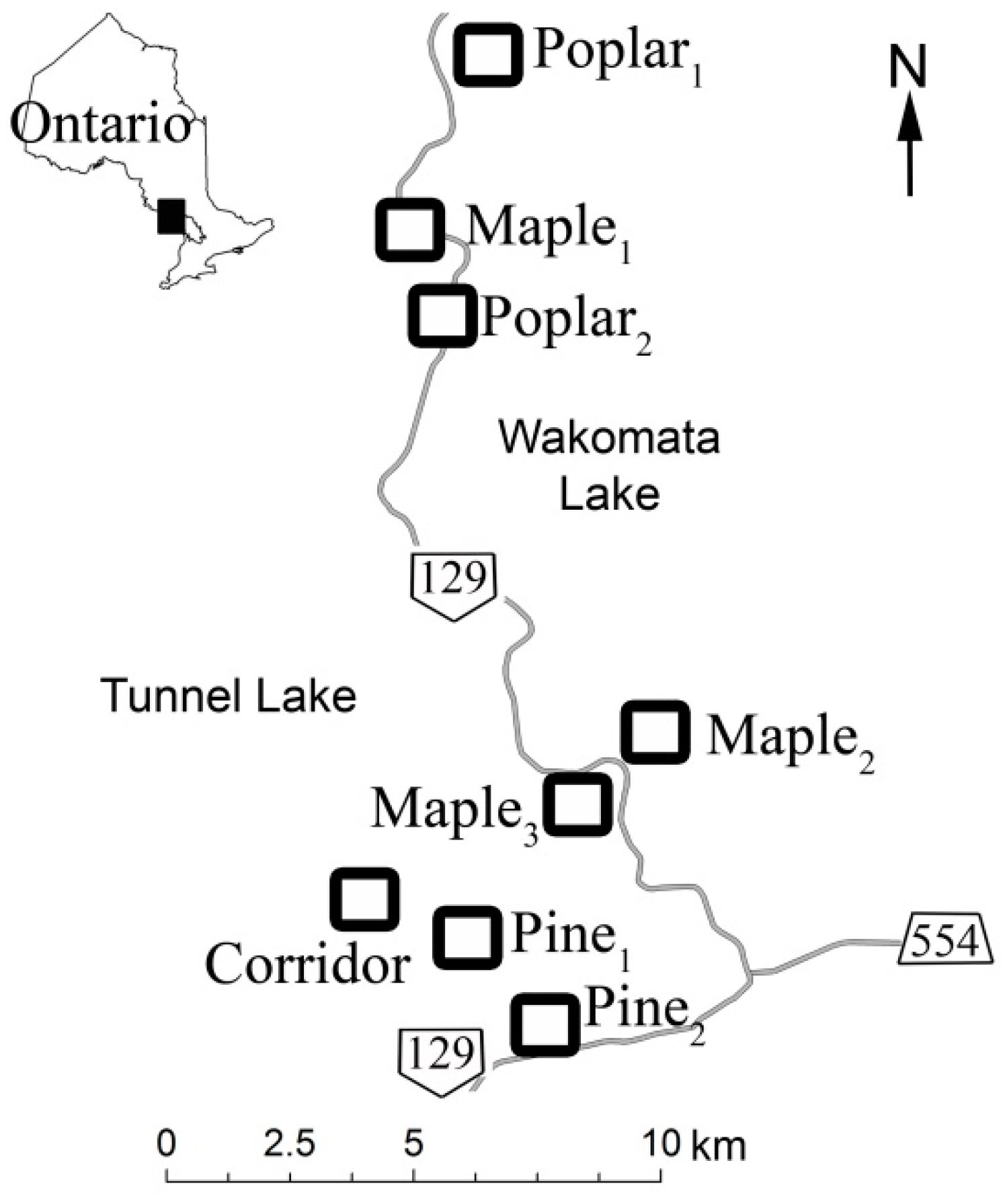
2. Study Area and Data

The field sites are located north of Thessalon, about 75 km east of Sault Ste. Marie, Ontario, Canada. There are eight field sites including one site along an electricity transmission line right-of-way (ROW) and seven other woodlots in the surrounding area named Poplar1, Poplar2, Maple1, Maple2, Maple3, Pine1, Pine2 and Corridor (Figure 1). During field validation performed between 30 July and 12 August 2009 and 8–10 August 2011, we identified white birch (Betula papyrifera Marsh.), balsam fir (Abies balsamea (L.)), sugar maple (Acer saccharum Marsh.), red oak (Quercus rubra L.), jack pine (Pinus banksiana Lamb.), trembling aspen (Populus tremuloides), white pine (Pinus strobus L.), and white spruce (Picea glauca (Moench Voss)). Tree height and dbh of each tree was measured; we also recorded the location of the tree using a handheld GPS for the verification of location in the LiDAR data. We field validated 189 trees, of which 160 belong to the genera of interest (pine, poplar and maple).
Figure 1. Map of the study area and the locations of the eight field survey sites.
Remotesensing 06 11225 g001
LiDAR data was collected on 7 August 2009 using a Riegl LMS-Q560 scanner; the flight altitude varied from 122∙m to 250 m above ground level. The pulse density is about 40 pulses∙m−2 with up to five returns per pulse. Individual trees were isolated from the LiDAR scene at the original pulse density and then the density of points was reduced to 20, 10, 5, 2.5 and 1.25 pulses∙m−2. Pulse return examples for pine, poplar, and maple trees for 40 and 1.25 pulses∙m−2 scans are shown in Figure 2.
Figure 2. Return distribution examples of maple (a) at 40 pulses∙m−2, maple (b) at 1.25 pulses∙m−2, pine (c) at 40 pulses∙m−2, pine (d) at 1.25 pulses∙m−2, poplar (e) trees at 40 pulses∙m−2 and poplar (f) trees at 1.25 pulses∙m−2.
Remotesensing 06 11225 g002

3. Methods

3.1. Overview of the Methodology

Geometric features were derived by clustering LiDAR point clouds that represent individual trees. The merging-splitting algorithm that groups representative points (belonging to a single branch) into a common cluster is described in [35], best-fit lines passing through each cluster centroid are drawn and the characteristics of those lines are calculated. The features also include metrics related to the convex hull of the LiDAR point cloud and 3D buffering of individual points. The second set of features (height attributes and intensity attributes) summarizes the properties of the vertical point distribution within each tree crown, including the mean, standard deviation, coefficient of variation, kurtosis and skewness of the height and intensity distribution for the entire crown. Each tree is height normalized and segmented into 10 slices stacked vertically. The 10th percentile features represent the LiDAR points belonging to the bottom 10th percentile of the tree crown height, whereas the 90th percentile features represents the points located at the top of the tree. Features include “first of many” returns, “single return” and “last of many” returns.
There are originally 24 geometric features and 78 vertical profile features derived for each tree. To reduce the model complexity and improve classification efficiency, the numbers of features were reduced to 6 and 26 respectively; the method of feature reduction is discussed in Section 2.3. By using Random Forests, LDA, kNN and SVM as the base classifiers, the classification was performed separately and then jointly. SVM is a supervised classifier that maximizes the distance from the data to the decision boundaries [19]. To train the data into kernel space, we have used the linear kernel function; the method we use to find the separating hyperplane is Sequential Minimal Optimization (SMO). The multiclass classifier was built based on a one-versus-all relation and to combine the base classifiers; the final decision was made by the largest number of votes.
The ensemble model uses a geometric classifier as the first classifier, followed by a combination of the geometric and vertical profile classifiers. In this paper, the relationship between classification accuracies and point density was also investigated by performing the classification with reduced point densities.

3.2. Random Forests

Random Forests itself is an ensemble classifier; it combines many classifications (categorical data) or regression trees (continuous data) for making a final labeling decision (class labels) [29,30] or predictions (values). The classification algorithm was implemented within the randomForest package for R [29,38]. In Random Forests, a certain portion (typically 37%) of training data is partitioned for estimating the classification accuracy and the partitioned data is called the out-of-bag (OOB) data, whereas using the rest of the data (in-bag) is used for tree construction. The importance of each feature can be calculated as follows: first, by estimating the OOB error from a classification tree, e; second, by random permutation the fth feature will produce a new OOB error ef; and third, by the MDA value for each feature, calculated by efe. This value is averaged over all trees and normalized by the standard deviation. If a feature has large MDA, it is a more important feature. Additionally, the proportion of vote and margin for each LiDAR tree were calculated and recorded. Some examples of remote sensing studies using Random Forests as classifiers are [39] for land type classification using LiDAR height and intensity metrics, [40] for crop classification and [28], which mapped seven types of forests using Random Forests with features derived from LiDAR and aerial photographs. Some studies compared the classification results with several classifiers, including Random Forests: Such as [26] classifying coniferous, deciduous, mixed and other classes with Random Forests, SVM and decision trees, and [41], which used Random Forests and SVM for studying the influence of spatial resolution on the derived maps. In this manuscript we focus our study using Random Forests and also compare results among LDA, kNN and SVM. Let X f be the features selected for classification, y be a predicted class label such that yL. According to [42], the binary indicator variable for voting the L instances with given X, can be written as p i ( y | X ) . Adapted from their notation, the average vote for a LiDAR tree to be assigned as one of the classes can be defined as Equation (1), the summation of all votes for the particular class divided by the number of classifiers (T) that make this decision:
V ( X ) = 1 T i = 1 T p i ( y | X ) ,   where  V L
The final label (y*) is decided by the majority voting (MV) scheme over T base classifiers described by Equation (2):
y * = M V ( X ) = argmax y L 1 T i = 1 T p i ( y | X )
For the partitioned training data, one can obtain the margin, described by [7] as:
M G ( X ) = 1 T i = 1 T p i ( y = Y | X ) max y Y [ 1 T i = 1 T p i ( y Y | X ) ]
The margin is defined as the distance from the data point to the decision boundary. In Random Forests, the margin is recorded as the proportion of votes for the correct class minus the maximum proportion of the incorrect classes. The larger the value of MG(X), the more confident one is of the correctness of the classification, whereas a negative margin indicates an incorrect prediction. Thus, the margin becomes an important indicator to evaluate the quality of label prediction provided by Random Forests. Such a post-evaluation of the label prediction often plays a key role to confirm or modify current decision outcomes in an iterative inference such as on-line learning [43], active learning [44], and combining multiple decision outcomes [45], as is discussed in our study.
The measurement of the margin requires the field-validated data or the reference data, Y. This makes MG only available for evaluating classification containing the reference information, and not applicable for evaluating the classification with prediction, where Y is normally not known prior to the classification. In order to assess the confidence of prediction without using the field validated data, we propose a new concept of pseudo-margin (PG). PG measures a degree of confidence in label prediction with unseen test data. Instead, PG assumes that the correct class label is supported by the maximum proportion of the vote (label prediction) and its confidence is evaluated by measuring the difference between the first and second majority votes using Equation (1). Thus, PG over the test sample X is now described as below:
P G ( X ) = max y L 1 T i = 1 T p i ( y | X ) second _ max y L 1 T i = 1 T p i ( y | X )
For our ensemble model, we use PG(X) for estimating the confidence of prediction instead of MG(X) to improve the usability of the model. To interpret PG(X), the larger the value, the more confidence can be placed on the prediction and the value of PG(X) will always be positive. This value will be used to filter out LiDAR trees that potentially exhibit incorrect classification from the first classifier and will be fully discussed in Section 2.4.
The main input parameters to Random Forests include: (1) labeled training samples, (2) the number of feature variables randomly sampled at each split (mtry = 2 for the geometric classifier and 5 for the vertical profile classifier), (3) the number of trees generated within each iteration (ntree = 1000 for this example), and (4) minimum size of terminal nodes (nodesize = 1 for this example). These values were set according to the suggestion from [38] where ntree is a large number; mtry ≈ square root of the number of feautres and nodesize = 1 is the default for classification trees. Random Forests produces the following output: (1) a ranking of each feature variable's importance calculated by MDA measured using OOB data, (2) a randomForest classification object for testing the validation data, and (3) vote and margin calculated for every LiDAR tree and class.

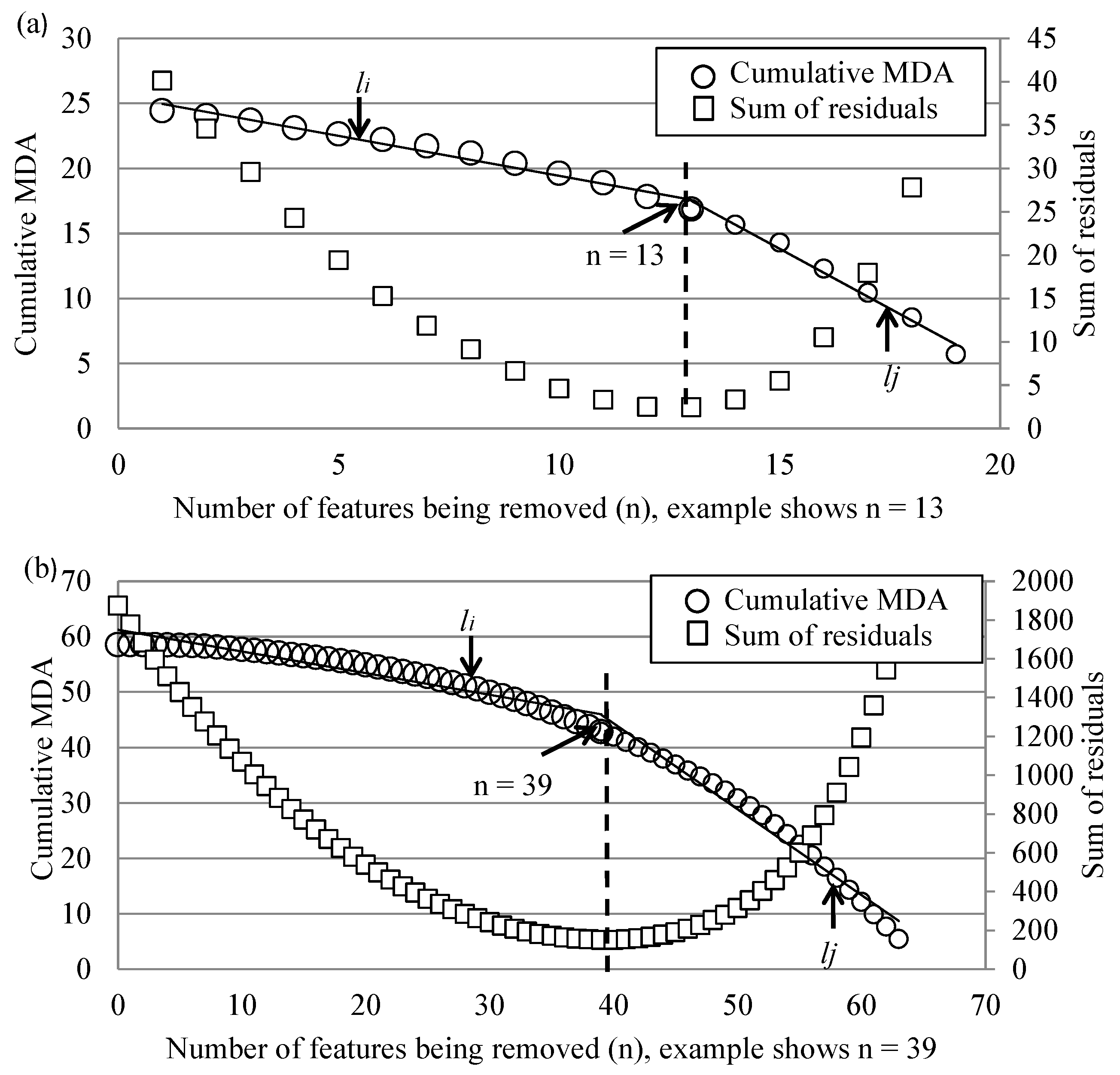
3.3. Feature Reduction

In order to simplify the base classifiers, the number of features was reduced by an automatic feature reduction method. Feature reduction for each classifier was performed in two steps. The first is to remove the highly correlated features to avoid issues of multi-collinearity. This initial reduction was conducted by calculating the pairwise correlation table and then removing features with r > 0.85, an empirically-determined threshold. The second step was performed in order to conduct a more rigorous feature reduction over the initial filtering results by Sequential Backward Selection (SBS) [46,47]. In SBS, a user-defined objective function J is needed to assess the performance of the feature subset; the optimal subset of features can be chosen by removing one least important feature at a time, starting with the full feature set until a single feature remains. By either maximizing or minimizing the objective function, the optimal number of features can be finally determined.
In our current study, SBS was modified to make it more suitable for the Random Forests applications by introducing a new objective function for optimally reducing the feature dimensionality. The goal of the objective function J is to determine the best partition between the number of features to be removed from the full feature set and the number of features which should remain. The MDA, discussed in Section 2.2, was employed as a criterion for identifying the optimum number of features chosen without a subjective cut-off in SBS.
All features were ranked in descending order, with which the cumulative MDA values were calculated separately for both geometric and vertical profile classifiers. Then, by removing one least important feature at a time, new cumulative MDA values can be obtained, until only one feature is left in each classifier. In the next step, we analyzed the changes in slopes of the cumulative MDA values by plotting them against the number of features being removed (circles in Figure 3). Both graphs (one for geometric features and one for vertical profile features) show that the cumulative MDA values decrease as the number of features removed increases. In both graphs, the decreasing rate increases because the important features are being removed later and at a certain point, the decreasing rate is abruptly changed when a significant feature starts to be eliminated. This property was adopted for the feature reduction.
Figure 3. Cumulative MDA (mean decrease accuracy) values for geometric classifiers (a) and cumulative MDA values for vertical profile classifiers (b); the residual sum of squares residual for fitting two linear lines through the cumulative MDA curve; dotted line shows where the residual sum of square minimizes. Solid lines represent li and lj at optimized J.
Remotesensing 06 11225 g003
The objective function J was derived from the fitting of two linear functions through each curve. The first line li regresses through the cumulative MDA values that are being removed from SBS, while, the second line lj will regresses through the cumulative MDA values remaining for each classifier. Let li be the linear function through the 1st to nth values and lj be the linear function through the nth to fth values such that Pi and Pj be the predicted MDA for the best fit line of li and lj. The rate of change for li and lj measures the relative importance of the removed feature with respect to the rest of the features. The optimum fitting was then found by minimizing the residual sum of squares from each point to the lines Equation (5), where the cumulative MDA measured at kth feature is denoted as A(k). The result of the analysis for the geometric classifier is shown in Figure 3a and result of the vertical profile classifier is shown in Figure 3b.
J = min ( i = 1 n ( P i A ( i ) ) 2 + j = n f ( P j A ( j ) ) 2 )
In Figure 3a, the result demonstrates that the best subset of features should be chosen when 13 features are removed (6 remaining) for the geometric classifier. In Figure 3b, the result demonstrates that the best subset of feature should be chosen when 39 features are removed (26 remaining) for the vertical profile classifier. The optimal number of features was chosen when the sum of residuals minimizes for both graphs, meaning this partition is best represented by two linear functions.

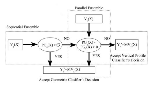
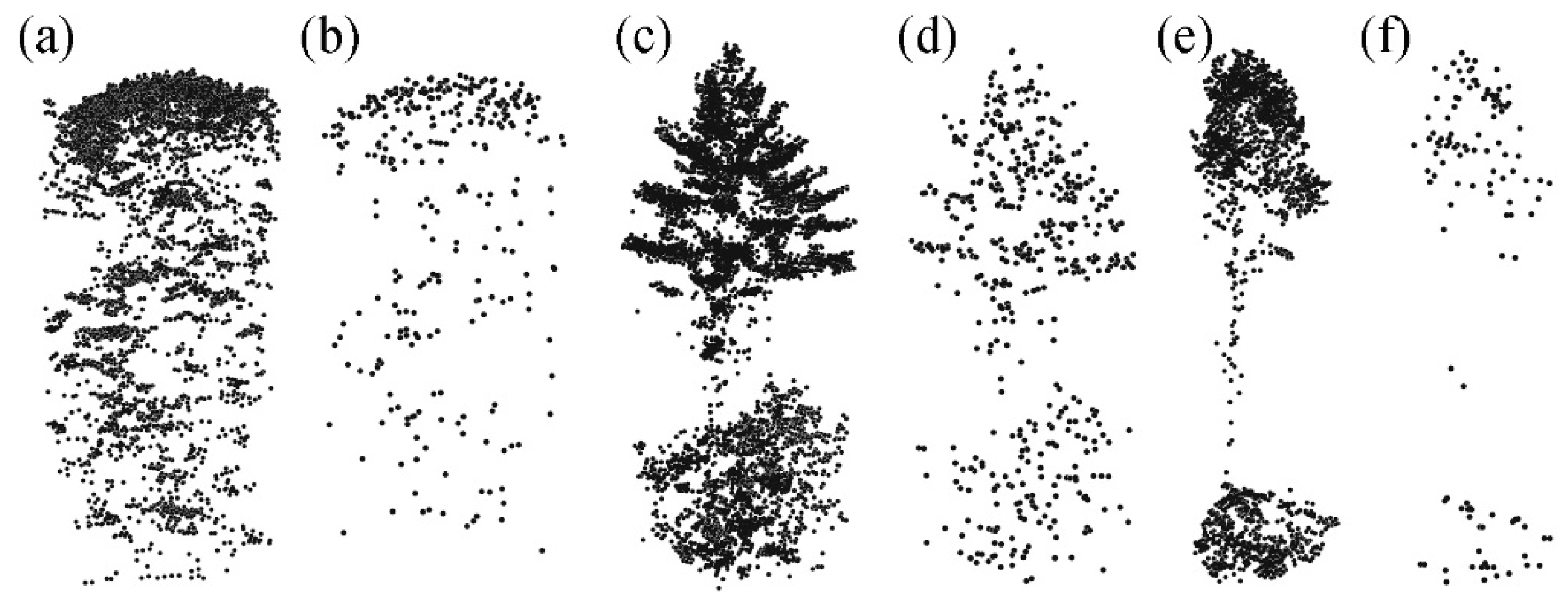
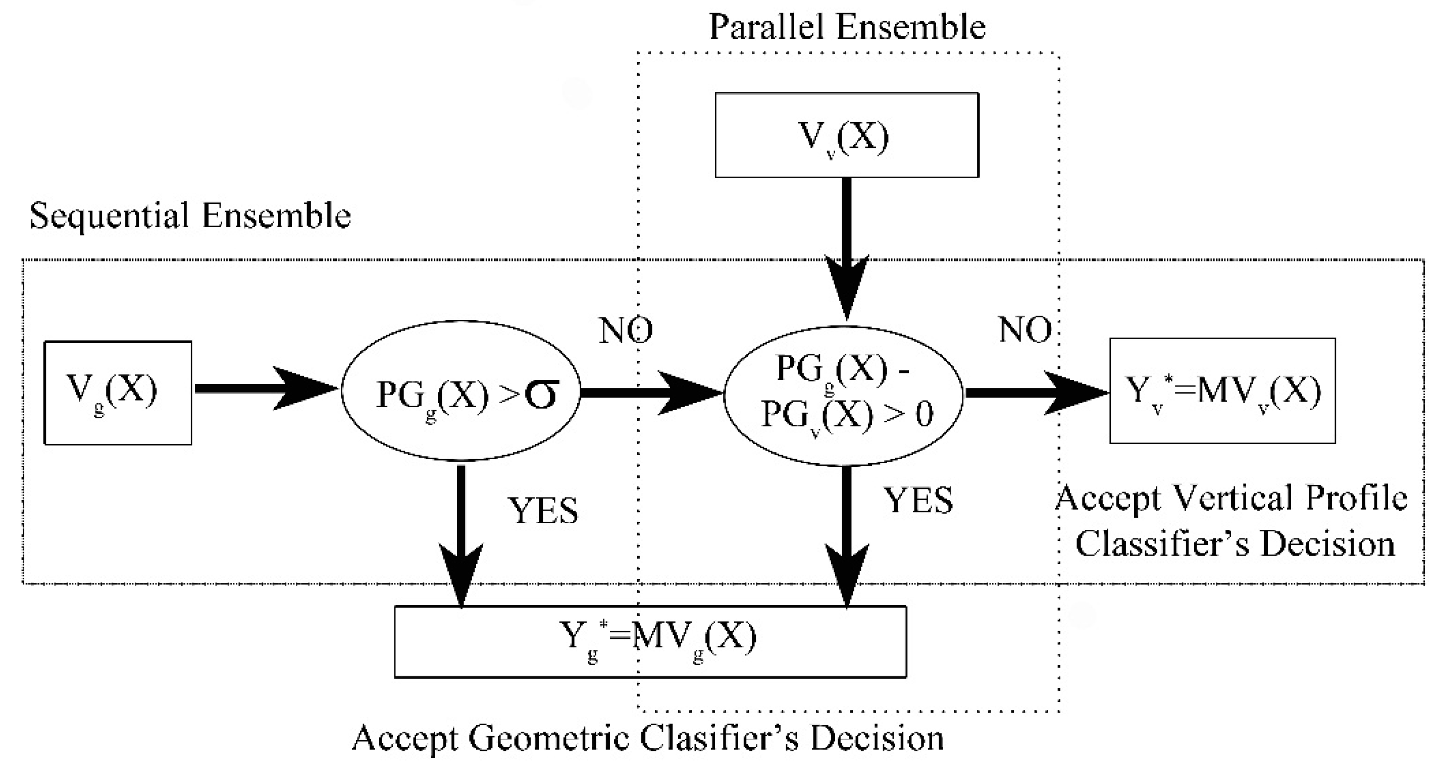
3.4. Geometric Classifier, Vertical Profile Classifier and Ensemble Methods

The objective of this section is to construct the ensemble classifier, jointly using sequential and parallel schemes. The ensemble classification combines the geometric features and vertical profile features and hence improves classification accuracy. Our model is dubbed a “hybrid ensemble” system because it combines the benefits of sequential and parallel approaches. As mentioned, the base classifier for this hybrid system is Random Forests; in Random Forests 25% of the randomly selected (stratified by class size) data were partitioned for training the classifier while the remaining data (75%) was partitioned for validation. This 25:75 ratio was chosen based on [35] and this process was repeated 20 times with 20 different sets of training and validation samples to achieve an average accuracy for each classifier. Figure 4 illustrates an overall workflow of the hybrid ensemble classification system.
First, the ensemble model was constructed to combine decisions sequentially and then in parallel. The reason for this two-step process was to minimize the amount of processing time when the number of samples is large. Instead of analyzing all the trees using two sets of features, trees that have higher prediction confidence will be filtered out and the decision made by the first classifier will be simply accepted. Hence, only the trees that are considered problematic will be classified using both classifiers, increasing the overall efficiency of the classification process. Therefore, the main objective of the first classifier is to filter out the trees that have a higher chance for misclassification and pass those to the second step. This step is performed by using a parameter σ from the PG(X) calculated from the testing data where σ is obtained from the distribution of MG(X) exhibited from the training data. This is an automated process and the estimation of σ is further discussed in section 2.5. The objective of the second classification procedure (parallel) is to combine decisions made from two classifiers for those filtered trees; the classifier with a higher calculated PG(X) will be responsible for the final decision (Figure 4). This second step considers both classifiers instead of simply taking the decision made by the second classifier, in case the first classifier is a better classifier; in that situation the final decision can be reverted.
Three experiments have been conducted in order to understand the hybrid ensemble system that has been developed. In the first experiment, classification accuracies are compared using the geometric classifier as the first classifier for filtering trees, followed by parallel ensemble classification as suggested in Figure 4, and using the vertical profile classifier as the first classifier, followed by parallel ensemble classification. The results for both experiments are elucidated in Table 5.
For the second experiment, the performances of different base classifiers are tested. Classification is performed using Random Forests, LDA, kNN and SVM with geometric features (geometric classifier) and vertical profile features (vertical profile classifier), separately and then combined. Features from each classifier are selected using the feature selection procedure (Section 2.3). However, the ensemble model that uses LDA, kNN and SVM as base classifiers is obtained from average voting rather than our proposed model, because the suggested ensemble model involves using the margins obtained from Random Forests (Equations (3) and (4)) that are not present in the LDA, kNN and SVM classifiers.
The third experiment explores the relationship between classification accuracies with the change in point density. The densities of individual trees are reduced by removing every other point (with respect to GPS time recorded by the scanner). Therefore, each LiDAR tree will have its original density level (40 pulses∙m2), and reduced to 20 pulses∙m2, 10 pulses∙m2, 5 pulses∙m2, 2.5 pulses∙m2 and 1.25 pulses∙m2. The classification procedures (individual classifiers, separately and jointly) are repeated for the different density levels. For each experiment and scenario, the ensemble processes are repeated 20 times and mean ensemble classification accuracy is obtained for each case.
Figure 4. Summary of the ensemble method using the geometric classifier as first classifier: MGg and MGv indicate the margin obtained from the geometric and the vertical profile classifiers, respectively; Vg and Vv represent the vote proportions obtained from the geometric and vertical profile classifiers, respectively; Yg* and Yv* correspond to the final predictions from geometric and vertical profile classifiers respectively.
Remotesensing 06 11225 g004

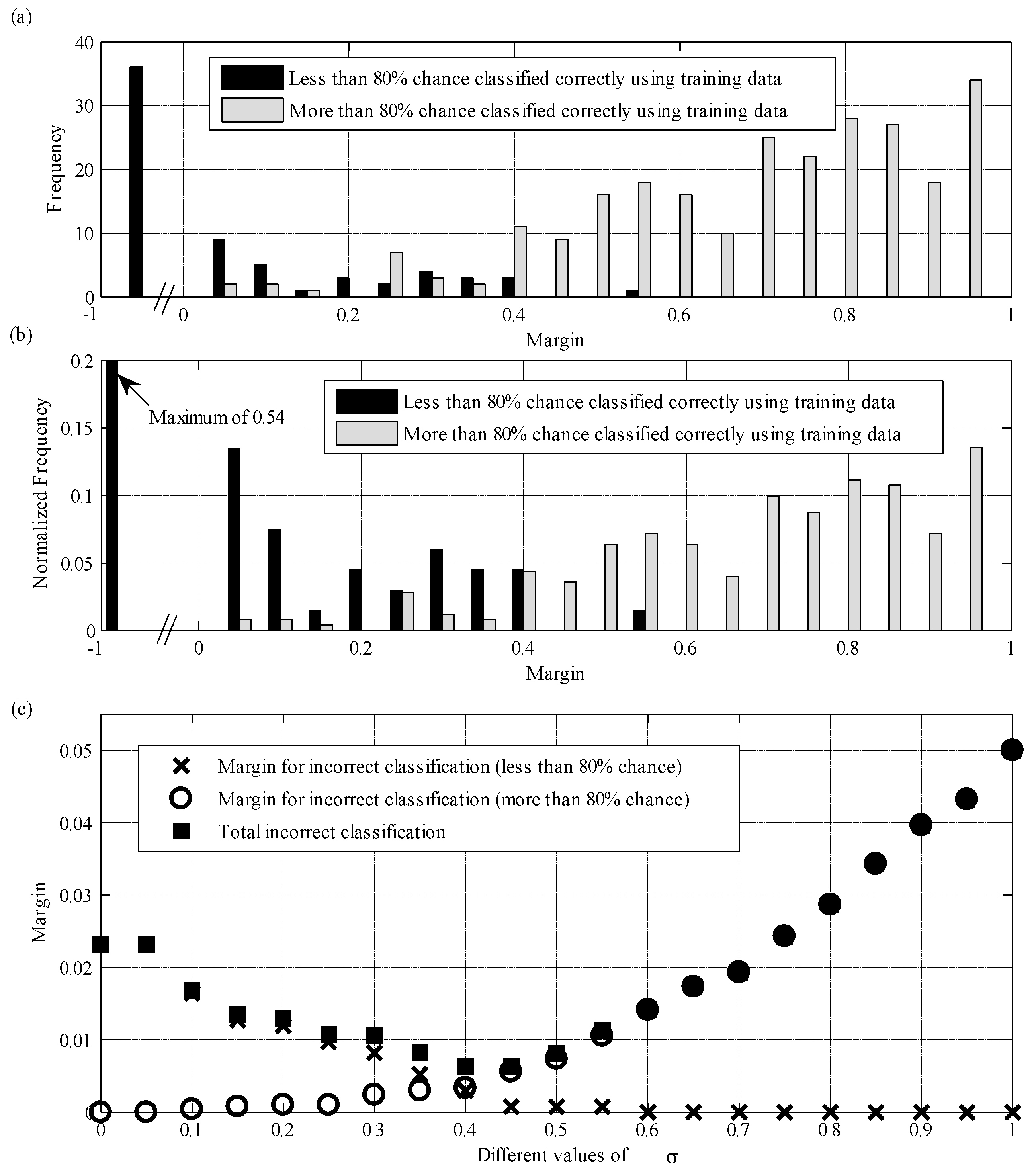
3.5. Parameter σ Estimation

As discussed in Section 2.4, σ is a parameter for separating trees that are selectively classified by different classification processes; it is a threshold designed for filtering the potential misclassified trees. The value for σ can range from 0 to 1; as σ approach 0, all trees will accept decisions made by the first classifier and none require a second classifier. Conversely, as σ approach 1, all trees will require the judgments from both classifiers.
In order to objectively and automatically decide on a threshold value, σ, from the training data, the following method is proposed. The MG(X) distribution of the training data is examined by plotting the frequency distribution of the margin calculated from the training data. To associate the relationship between MG(X) and classification accuracy, the distribution is classified into two groups using 80% as an example displayed in Figure 5a. To interpret the 80%—it is the acceptable estimated classification accuracy for filtering trees from the first classifier in Figure 4. By changing this value the margin distribution in Figure 5a will not change since the margin distribution is independent of acceptable classification accuracy, rather how it is being grouped (the black and grey bars) will alter. Figure 5a shows the frequency distribution of MG(X) calculated from the training samples, grouped by correctly classified for at least 80% (and less than 80%) with 20 randomly selected sample subsets.
The goal of making this plot is to select an optimal margin value σ that best separates between these two groups and uses this value for filtering. The two groups from Figure 5a are treated as two different distributions and normalized by the total frequency. This is done because the total frequency count of the less-than-80%-chance-correctly-classified group is much less than the more-than-80%-chance-correctly-classified group. However, both distributions have been treated as equally important. Using Figure 5b, the optimal σ is chosen by treating this graph as a binary classification problem using a threshold. The optimal partition is estimated by testing different values of σ so that the total incorrect margin (frequency × width of the histogram bar) is minimized-tested over different σ values. For example, if σ = 0.25, the black bars with values larger than 0.25 correspond to a margin for incorrect classification (less than 80% chance) and the grey bars with values smaller than 0.45 correspond to a margin for incorrect classification (more than 80% chance). The total incorrect classification is the sum of these two values. Using this method, σ = 0, 0.05, …, 1.00 is tested and the margin for incorrect classification for each σ is recorded with the objective to minimize the total incorrect margin. Figure 5c shows that the total incorrect classification minimizes at σ = 0.45 with this given dataset.
Figure 5. Frequency distribution of the LiDAR (Light Detection and Ranging) trees that are correctly classified for at least 80% (and less than 80%) with 20 randomly selected sample subsets (a). Normalized frequency distribution of (a) is shown in (b). Margin for incorrect classification (for more and less than 80% chance) and total margin for incorrect classification at different σ (c).
Remotesensing 06 11225 g005

4. Results and Discussion

In this paper, an ensemble method is employed to combine features derived from the geometry of LiDAR points reflected from individual trees with features derived from vertical point distribution. The advantage of using geometric features is that these features relate closely to the biophysical interpretation of trees, with the advantage of vertical profile that they are computationally simple. The proposed classification method is useful in many environmental applications since genera identification is one of the most critical parameters, especially when performing an inventory of the individual tree resolution. Examples of applications include supplementing information for existing forest inventories and for commercial or non-commercial forest management purposes. Improved classification accuracies also improve estimates of forest parameters such as for carbon budgets and biomass volumes. Also, our method can be useful in vegetation management near human infrastructure, or for urban planning purposes.

4.1. Selected Feature Tables

From the feature reduction experiment using the geometric classifier, the numbers of features have been reduced from 24 to 6 and from 78 to 26 for the vertical profile classifier. The list of selected geometric classifier features are shown in Table 1 and the list of selected vertical profile classifier features are shown in Table 2.
Table 1. List of selected geometric features.
No. Description
F1Average derived best bit line segment lengths divided by tree height
F2 Average line segment lengths multiplied by the ratio between tree crown height and tree height
F3 Volume of the tree crown convex hull divided by the number of points in the crown
F4Average distance from each point to the closest facet of the convex hull
F5Buffer each LiDAR point outward at a radius of 2% of the tree height, calculate the overlapped volume of the spheres divided by the number of points in the tree crown
F6Tree crown height divided by the tree height
Table 2. List of selected vertical profile features, F = first; S = single; L = last; SD = standard deviation; CV = coefficient of variation.
10th Percentile50th Percentile90th Percentile
% of canopy return (V1S, V2L)
% return count (V3F, V4S, V5L) % return count(V6F, V7S, V8L)
Mean height of canopy return (V9F, V10L)
SD of height (V11F, V12S)
SD height for canopy return (V13F, V14L)
CV height for canopy return (V15F, V16S)
Kurtosis of variation height for canopy return (V17S, V18L)
Skewness of variation height for canopy return (V19S, V20L)
Mean intensity (V21L) Mean intensity (V22F, V23S)
SD of intensity (V24F)
CV intensity of canopy return (V25L)
Skewness of variation intensity of canopy return (V26S)

4.2. Classification Performance

By using Random Forests as a base classifier, the classification accuracies using geometric features and vertical profile features separately are 88.0% and 88.8%, respectively. When the base classifier is replaced by LDA, the classification accuracies are 85.6% and 78.0%, if replaced by kNN, the classification accuracies are 85.3% and 70.9%, and if replaced by SVM, the classification accuracies are 79.1% and 80.4% when using geometric and vertical profile features independently. The classification accuracy improves to 91.2% using the ensemble method when running Random Forests as the base classifier and using the geometric classifier first for filtering LiDAR trees; the classification accuracy is 90.3% when vertical profile classifier is run first. The ensemble classification accuracy from LDA is 89.4%, 85.6% if kNN is being used and 88.7% if SVM is being used. The results are summarized in Table 3.
The classification accuracies from using geometric features alone is lowest in SVM and highest in Random Forests, the classification accuracies from using vertical profile alone is lowest in kNN and highest in Random Forests. Random Forests produces the best results over all other classification scenarios when geometric or vertical features are used independently or jointly in our ensemble classification. All four methods indicate that by combining both feature classes, the classification accuracy can be increased. The comparison of classification accuracies among different base classifiers (Random Forests, LDA, kNN, and SVM) indicates that Random Forests is an efficient classifier that outperforms the other three.
Table 3. Classification accuracies (%) with using different base classifiers.
GeometricVerticalEnsemble
Random Forests88.088.891.2
LDA85.678.089.4
kNN85.370.985.6
SVM79.180.488.7
With a focus on the analyses using Random Forests as the base classifier, the confusion matrix for classification by geometric and vertical profile is provided in Table 4. The confusion matrix for the ensemble classification results is shown in Table 5. The confusion matrices are computed by using 75% of the 160 LiDAR trees for classification, repeated 20 times, with results of 2400 trees assessed.
When individual classifiers are compared (Table 4), both classifiers have the largest errors when trying to separate pine from poplar; this is attributed to the similarity between the vertical point distributions for pine and poplar, with points located mostly at the top of the tree crown. For the geometric classifier, the ratio between the tree crown height and tree height for both genera are also similar, again resulting in confusion. Conversely, highest accuracy is observed in maple classification by both classifiers.
By comparing the results from the geometric classifier alone with the ensemble classification using the geometric classifier as the first classifier and results from the vertical profile classifier alone with the ensemble classification using the vertical profile classifier as the first classifier (Table 4 and Table 5), accuracies for all genera are improved (except for producer’s accuracy for maple; vertical profile classifier). This implies that using the margin and pseudo-margin is effective for automatically filtering out LiDAR trees that are difficult to classify by the first classifier. The improvements in accuracies also suggest that the ensemble method outperforms the single classifier alone. Table 4 shows that individual classifiers (geometric features and vertical profile features) differ in their classification decisions; for example, the producer’s accuracy for pine has the largest difference. The differences indicate that there is potential for improving the accuracy after combining the classifiers.
Table 4. Confusion matrix for individual classifier: bold number: geometric classifier (average accuracy of 88.0%); italic numbers: vertical profile classifier (average accuracy of 88.8%).
ExpectedUser’s Accuracy (%)
PinePoplarMaple
PredictedPine856906115132191286.586.3
Poplar123877717362786.088.7
Maple271311948648894.693.8
Producer’s Accuracy (%)85.190.186.983.095.996.3
Table 5. Confusion matrix for ensemble classification, Bold number: geometric classifier as first classifier (average accuracy of 91.2%); italic numbers: vertical profile classifier as first classifier (average accuracy of 90.3%).
ExpectedUser’s Accuracy (%)
PinePoplarMaple
PredictedPine9039089410952190.187.5
Poplar86807867773589.890.1
Maple17187149948195.496.2
Producer’s Accuracy (%)89.890.388.687.698.494.9
By combining the decisions made by the two classifiers, the classification accuracy improved from 88.0% to 91.2% if the geometric classifier is being used as the first classifier and 88.8% to 90.3% if the vertical profile classifier is being used as the first classifier (Table 5). Since the original accuracies (with the single classifier alone) are trade high, the marginal improvement that we achieve is impressive. Although the most common way of assessing classifiers is the classification accuracy, the benefits of ensemble classification is beyond the increase in classification accuracy. Ensemble classification allows the utilization of different training data types to better suit the individual base classifier. Identical tree genera can appear different simply due to varied environmental or site conditions (e.g., an open windy environment versus a closed forest with lots of overlapping tree crowns).

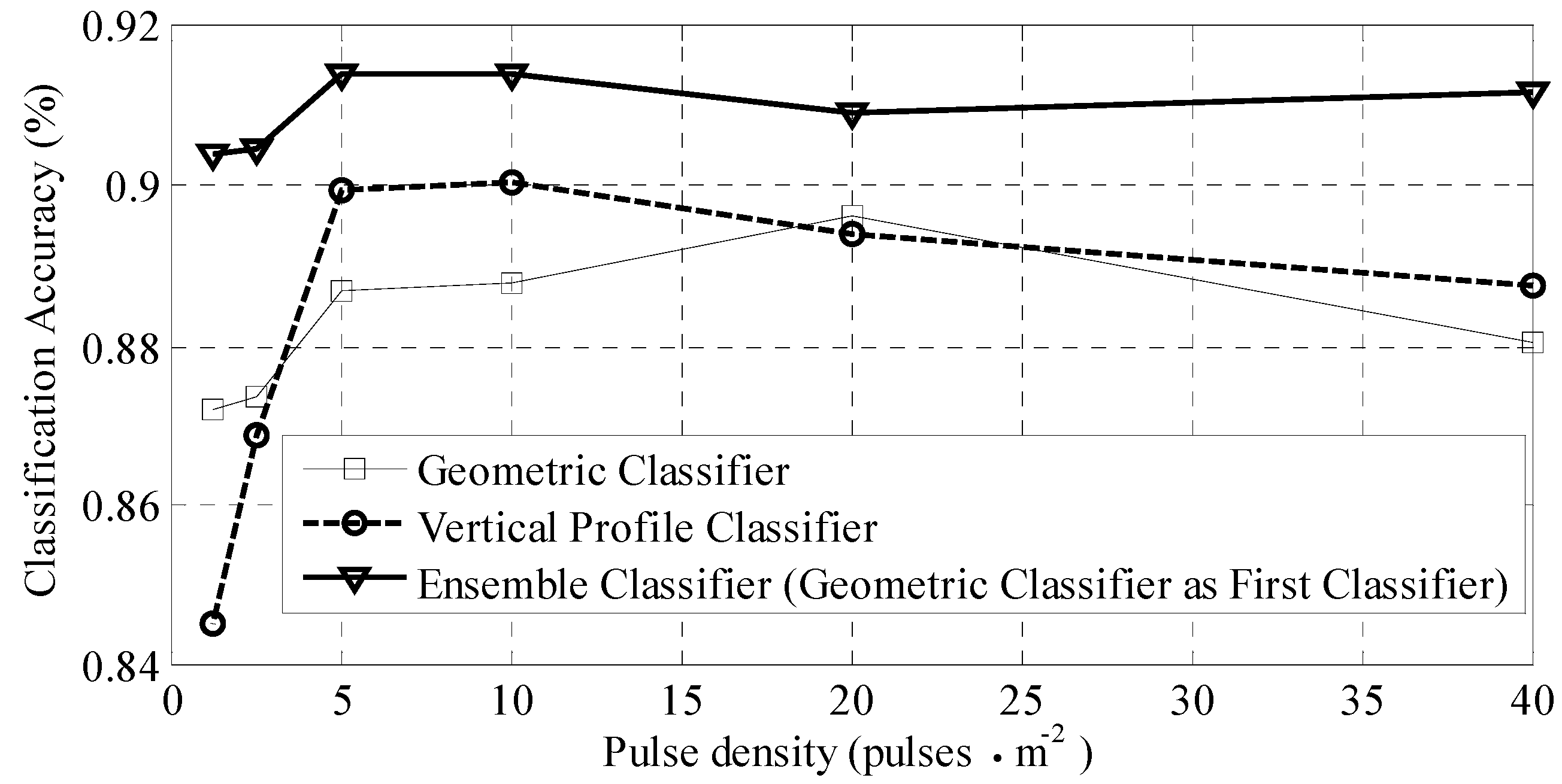
4.3. Results from Point Density Analysis

The relationship between classification accuracy with different pulse densities is shown in Figure 6, with error bars showing the standard error for each point within the 20 trials. For all classifiers, the accuracy stays at about the same level for 40, 20 and 10 pulses∙m−2, and then begins decreasing at 5, 2.5 and 1.25 pulses∙m−2. The geometric classifier and vertical classifier show similar results for all density levels except at 1.25 pulses∙m−2, where the accuracy for vertical profile classifier is 3% lower than geometric classifier. Also, ensemble classification shows higher classification accuracy at all density levels. It can be concluded that there are opportunities to reduce the pulse density to 10 or 5 pulses∙m−2, resulting in lower costs in data acquisition and processing handling for comparable results, although the tradeoff between classification accuracy and pulse density will need to be considered if the pulse densities decrease further. Two one-tailed t-tests were conducted to verify that the increase in classification accuracies resulted from ensemble classification is statistically significant. One t-test examines the relationship between geometric classifier to ensemble classification and the other t-test examines the relationship between vertical profile classifier to ensemble classification. There was a significant difference in the scores for geometric classifier (M = 0.88, SD = 0.01) and ensemble classifier (M = 0.91, SD = 4.49 × 10⁻³); t(10) = −6.37, p = 4.07 × 10⁻⁵). There was also a significant difference in the scores for vertical profile classifier (M = 0.88, SD = 0.02) and ensemble classifier (M = 0.91, SD = 4.49 × 10⁻³); t(10) = −2.99, p = 6.71 × 10⁻³).
Figure 6. Classification accuracy of the geometric, vertical profile, and ensemble classifiers, using the geometric classifier as the first classifier at different LiDAR pulse density levels.
Remotesensing 06 11225 g006
In order to study the performance of the classifiers with the reduction of LiDAR point density, an experiment studying the relationship between classification accuracy and point density was performed. Results showed that similar classification accuracy can be obtained at lower density levels (down to 5 pulses∙m−2) and accuracy dropped for individual classifiers and for the ensemble classifier when the density level was lower than 5 pulses∙m−2. This indicated that there is a trade-off between classification accuracy and pulse density; however, the trade-off is higher when the pulse density falls beyond 5 pulses∙m−2. This result shows there is room for reducing the pulse density to trade for slightly lower classification accuracy, and this normally results in lower costs.

5. Conclusions

The three major contributions of this paper include first, the implementation of an automatic feature reduction method that utilizes the results obtained from Random Forests. Feature reduction is an important procedure to avoid overfitting and keeping the final classification model realistically parsimonious. Many of the remote sensing studies that use Random Forests as a classifier did not perform this analysis [19,22,26,40,41], and some use a fixed threshold (e.g., [7] and [25]). There are two advantages of using an optimization method to reduce the number of features, the first is to avoid the subjectivity compared to the use of a threshold, the second is to avoid the problem of identifying effective thresholds for each new dataset to be analyzed.
The second contribution of this paper is the use of the pseudo-margin for estimating the quality of prediction, where the pseudo-margin is derived from the margin. Margin measures the distance of a sample away from the decision boundary and is therefore useful to assess the confidence of prediction. However, the measurement of the margin requires prior knowledge of the species label. Hence, we developed pseudo-margin that does not require the prior knowledge and is suitable to use for prediction. During the prediction process, σ (a pseudo-margin value) is used for separating trees with higher prediction confidence from those with lower prediction confidence, and this value is optimally estimated by analyzing the margin distribution of training data. Also, the pseudo-margin is also used in the parallel part of the model for making the final decision.
The third contribution involves the development and application of a hybrid ensemble classification system for improving overall classification accuracies. Instead of using the traditional parallel or sequential ensemble system, we have designed a hybrid system that overcomes some traditional limitations. When building a parallel model, all features from all classifiers have to be derived; however, by using one of the classifiers to filter out trees that have high prediction confidence a priori, a smaller subset of classifications is necessary and workload is substantially reduced. Moreover, when compared to a pure sequential model, this hybrid model also benefits from being able to revert decisions. When ensemble models are designed sequentially, decisions made by the first classifier are passed to the second model and the second classifier makes the decision (assuming there are only two classifiers), yet, the performance of the classifier differs for each sample and the final classifier in the sequence does not always make the best decision. Our hybrid system incorporates a parallel system within the sequential framework such that in the second step, a comparison between the two classifiers is made and if the first classifier has a higher prediction confidence, the final decision can be made by the first classifier.
The overall goal of this work is to improve the classification accuracies from a single classification model. Our results showed that it is possible to improve classification accuracy by using an ensemble classification system with overall classification accuracy increases observed from 88.0% to 91.2%. Although the sample size for this research is limited, the design of the hybrid system is suitable for the classification of large amounts of data. Instead of classifying all trees with two classifiers, the first classifier intelligently selects trees that have higher prediction confidence and makes final classification decisions at that point. Only the lower prediction confidence samples are judged by two classifiers. Ensemble classification allows for flexibility in combining classifiers, and in the future additional feature types can easily be integrated into this framework as extra base classifiers, forming a modular classification design.

Acknowledgments

This research was funded by GeoDigital International Inc., Ontario Centres for Excellence, and a Discovery Grant from the Natural Sciences and Engineering Research Council of Canada. We thanks Richard Pollock, Konstantin Lisitsyn, Doug Parent, and Yulia Lazukova at GeoDigital International Inc. for their assistance in preparing the data; Junji Zhang, Jili Li, Yoonseok Jwa at York University, Canada, and Nakhyn Song at Inha University, South Korea for acquiring field surveying data for this study.

Author Contributions

Connie Ko, Gunho Sohn, Tarmo K. Remmel and John Miller wrote and edited the manuscript. Connie Ko designed and implemented the experiments with the advice of Gunho Sohn and Tarmo K. Remmel. All authors discussed the results, discussions of the manuscript.

Conflicts of Interest

The authors declare no conflicts of interest.

References

  1. Clark, M.L.; Roberts, D.A.; Clark, D.B. Hyperspectral discrimination of tropical rain forest tree species at leaf to crown scales. Remote Sens. Environ. 2005, 96, 375–398. [Google Scholar] [CrossRef]
  2. Cochrane, M.A. Using vegetation reflectance variability for species level classification of hyperspectral data. Int. J. Remote Sens. 2000, 21, 2075–2087. [Google Scholar] [CrossRef]
  3. Holmgren, J.; Persson, A. Identifying species of individual trees using airborne laser scanning. Remote Sens. Environ. 2004, 90, 415–423. [Google Scholar] [CrossRef]
  4. Barilotti, A.; Crosilla, F.; Sepic, F. Curvature Analysis of LiDAR Data for Single Tree Species Classification in Alpine Latitude Forests. Available online: http://www.isprs.org/proceedings/xxxviii/3-w8/papers/129_laserscanning09.pdf (accessed on 12 September 2009).
  5. Brandtberg, T. Classifying individual tree species under leaf-off and leaf-on conditions using airborne LIDAR. ISPRS J. Photogramm. Remote Sens. 2007, 61, 325–340. [Google Scholar] [CrossRef]
  6. Kato, A.; Moskal, L.M.; Schiess, P.; Swanson, M.E.; Calhoun, D.; Stuetzle, W. Capturing tree crown formation through implicit surface reconstruction using airborne LIDAR data. Remote Sens. Environ. 2009, 113, 1148–1162. [Google Scholar] [CrossRef]
  7. Mellor, A.; Haywood, A.; Stone, C.; Jones, S. The performance of random forests in an operational setting for large area sclerophyll forest classification. Remote Sens. 2013, 5, 2838–2856. [Google Scholar] [CrossRef]
  8. Ørka, H.O.; Næsset, E.; Bollandsås, O.M. Utilizing Airborne Laser Intensity for Tree Species Classification. Available online: http://www.isprs.org/proceedings/XXXVI/3-W52/final_papers/Oerka_2007.pdf (accessed on 14 September 2007).
  9. Korpela, I.; Ørka, H.O.; Maltamo, M.; Tokola, T. Tree species classification using airborne LiDAR—Effects of stand and tree parameters, downsizing of training set, intensity normalization and sensor type. Silva Fenn. 2010, 44, 319–339. [Google Scholar] [CrossRef]
  10. Kim, S.; Hinckley, T.; Briggs, D. Classifying individual tree genera using stepwise cluster analysis based on height and intensity metrics derived from airborne laser scanner data. Remote Sens. Environ. 2011, 115, 3329–3342. [Google Scholar] [CrossRef]
  11. Samadzadegan, F.; Bigdeli, B.; Ramzi, P. A multiple classifier system for classification of LIDAR remote sensing data using multi-class SVM. Multi. Classif. Syst. 2010, 5997, 254–263. [Google Scholar]
  12. Ruta, D.; Gabrys, B. An overview of classifier fusion methods. Comp. Inf. Sys. 2000, 7, 1–10. [Google Scholar]
  13. Zhou, Z.H. Ensemble Methods: Foundations and Algorithms (Chapman & Hall/CRC Machine Learning & Pattern Recognition); CRC Press: Boca Raton, FL, USA, 2012. [Google Scholar]
  14. Briem, G.J.; Benediktsson, J.A.; Sveinsson, J.R. Multiple classifiers applied to multisource remote sensing data. IEEE Trans. Geosci. Remote Sens. 2002, 40, 2291–2299. [Google Scholar] [CrossRef]
  15. Palmason, J.A.; Benediktsson, J.A.; Sveinsson, J.R.; Chanussot, J. Fusion of Morphological and Spectral Information for Classification of Hyperspectral Urban Remote Sensing Data. Available online: http://www.gipsa-lab.grenoble-inp.fr/~jocelyn.chanussot/publis/ieee_igarss_06_palmason_fusionhyper.pdf (accessed on 4 September 2014).
  16. Breiman, L. Bagging predictors. Mach. Learn. 1996, 24, 123–140. [Google Scholar]
  17. Dietterich, T.G. An experimental comparison of three methods for constructing ensembles of decision trees: Bagging, boosting and randomization. Mach. Learn. 2000, 40, 139–158. [Google Scholar] [CrossRef]
  18. Freund, Y.; Schapire, R.E. A decision-theoretic generalization of on-line learning and an application to boosting. J. Comput. System Sci. 1997, 55, 119–139. [Google Scholar] [CrossRef]
  19. Cortes, C.; Vapnik, V. Support-vector networks. Mach. Learn. 1995, 20, 273–297. [Google Scholar]
  20. Ghimire, B.; Rogan, J.; Rodriguez-Galiano, V.F.; Panday, P.; Neeti, N. An evaluation of bagging, boosting, and random forests for land-cover classification in Cape Cod, Massachusetts, USA. GISci. Remote Sens. 2012, 49, 623–643. [Google Scholar] [CrossRef]
  21. Dettling, M. Bagboosting for tumor classification with gene expression data. Bioinformatics 2004, 20, 3583–3593. [Google Scholar] [CrossRef] [PubMed]
  22. Ali, K.M.; Pazzani, M.J. Error reduction through learning multiple descriptions. Mach. Learn. 1996, 24, 173–202. [Google Scholar]
  23. Breiman, L. Arcing classifiers. Ann. Stat. 1998, 26, 801–824. [Google Scholar] [CrossRef]
  24. Kavzoglu, T.; Colkesen, I. An assessment of the effectiveness of a rotation forest ensemble for land-use and land-cover mapping. Int. J. Remote Sens. 2013, 34, 4224–4241. [Google Scholar] [CrossRef]
  25. Engler, R.; Waser, L.T.; Zimmermann, N.E.; Schaub, M.; Berdos, S.; Ginzler, C; Psomas, A. Combining ensemble modeling and remote sensing for mapping individual tree species at high spatial resolution. Forest Ecol. Manag. 2013, 310, 64–73. [Google Scholar] [CrossRef]
  26. Li, M; Im, J.; Beier, C. Machine learning approaches for forest classification and change analysis using multi-temporal Landsat TM images over Hungtington Wildlife Forest. GISci. Remote Sens. 2013, 50, 361–384. [Google Scholar]
  27. Kumar, S.; Ghosh, J.; Crawford, M.M. Hierarchical fusion of multiple classifiers for hyperspectral data analysis. Pattern Anal. Appl. 2002, 5, 210–220. [Google Scholar] [CrossRef]
  28. Zhang, C.; Xie, Z.; Selch, D. Fusing LIDAR and digital aerial photography for object-based forest mapping in the Florida Everglades. GISci. Remote Sens. 2013, 50, 562–573. [Google Scholar]
  29. Breiman, L. Random forests. Mach. Learn. 2001, 45, 5–32. [Google Scholar] [CrossRef]
  30. Liaw, A.; Wiener, M. Classification and regression by random Forest. R. News. 2002, 2, 18–22. [Google Scholar]
  31. Vauhkonen, J.; Korpela, I.; Maltamo, M.; Tokola, T. Imputation of single-tree attributes using airborne laser scanning-based height, intensity, and alpha shape metrics. Remote Sens. Environ. 2010, 114, 1263–1276. [Google Scholar] [CrossRef]
  32. Vauhkonen, J.; Tokola, T.; Maltamo, M.; Packalen, P. Effects of pulse density on predicting characteristics of individual trees of Scandinavian commercial species using alpha shape metrics based on ALS data. Can. J. Remote Sens. 2008, 34, S441–S459. [Google Scholar] [CrossRef]
  33. Vauhkonen, J.; Tokola, T.; Packalen, P.; Maltamo, M. Identification of Scandinavian commercial species of individual trees from airborne laser scanning data using alpha shape metrics. Forest Sci. 2009, 55, 37–47. [Google Scholar]
  34. Ørka, H.O.; Næsset, E.; Bollandsås, O.M. Classifying species of individual trees by intensity and structure features derived from airborne laser scanner data. Remote Sens. Environ. 2009, 113, 1163–1174. [Google Scholar] [CrossRef]
  35. Ko, C.; Sohn, G.; Remmel, T.K. Tree genera classification with geometric features from high-density airborne LiDAR. Can. J. Remote Sens. 2013, 39, S73–S85. [Google Scholar] [CrossRef]
  36. Ko, C.; Sohn, G.; Remmel, T.K. A comparative study using geometric and vertical profile features derived from airborne LiDAR for classifying tree genera. Available online: http://www.isprs-ann-photogramm-remote-sens-spatial-inf-sci.net/I-3/129/2012/isprsannals-I-3-129-2012.pdf (accessed on 5 August–1 September 2012).
  37. Magnusson, M.; Fransson, J.E.S.; Holmgren, J. Effects on estimation accuracy of forest variables using different pulse density of laser data. Forest Sci. 2007, 53, 619–626. [Google Scholar]
  38. R Development Core Team. R: A Language and Environment for Statistical Computing. Available online: http://www.R-project.org/ (accessed on 5 September 2014).
  39. Alexander, C.; Bøchera, P.K.; Arge, L.; Svenning, J.C. Regional-scale mapping of tree cover, height and main phenological tree types using airborne laser scanning data. Remote Sens. Environ. 2014, 147, 156–172. [Google Scholar] [CrossRef]
  40. Long, J.A.; Lawrence, R.L; Greenwood, M.C.; Marshall, L.; Miller, P.R. Object-oriented crop classification using multitemporal ETM+ SLC-off imagery. GISci. Remote Sens. 2013, 50, 418–436. [Google Scholar]
  41. Ghosh, A.; Fassnacht, F.E.; Joshi, P.K.; Koch, B. A framework for mapping tree species combining hyperspectral and LiDAR data: Role of selected classifiers and sensor across three spatial scales. Int. J. Appl. Earth Obs. Geoinf. 2014, 26, 49–63. [Google Scholar] [CrossRef]
  42. Schwing, A.; Zach, C.; Zheng, Y.; Pollefeys, M. Adaptive Random Forest—How Many “Experts” to Ask before Making a Decision. Available online: http://alexander-schwing.de/papers/SchwingEtAl_CVPR2011b.pdf (accessed on 5 September 2014).
  43. Hinton, G.E.; Osindero, S.; Teh, Y.W. A fast learning algorithm for deep belief nets. Neural Comput. 2006, 18, 1527–1554. [Google Scholar] [CrossRef] [PubMed]
  44. Tong, S.; Koller, D. Support vector machine active learning with applications to text classification. J. Mach. Learn. Res. 2002, 2, 45–66. [Google Scholar]
  45. Rokach, L. Ensemble-based classifiers. Artif. Intell. Rev. 2010, 33, 1–39. [Google Scholar] [CrossRef]
  46. Jain, A.; Zongker, D. Feature selection: Evaluation, application, and small sample performance. IEEE Trans. Pattern Anal. 1997, 19, 153–158. [Google Scholar] [CrossRef]
  47. Serpico, S.B.; D’Inca, M.; Melgani, F.; Moser, G. A Comparison of Feature Reduction Techniques for Classification of Hyperspectral Remote Sensing Data. Available online: http://www.researchgate.net/publication/253371695_Comparison_of_feature_reduction_techniques_for_classification_of_hyperspectral_remote_sensing_data (accessed on 5 September 2014).

