Multisensor NDVI-Based Monitoring of the Tundra-Taiga Interface (Mealy Mountains, Labrador, Canada)

Abstract
: The analysis of a series of five normalized difference vegetation index (NDVI) images produced information about a Labrador (Canada) portion of the tundra-taiga interface. The twenty-five year observation period ranges from 1983 to 2008. The series composed of Landsat, SPOT and ASTER images, provided insight into regional scale characteristics of the tundra-taiga interface that is usually monitored from coarse resolution images. The image set was analyzed by considering an ordinal classification of the NDVI to account for the cumulative effect of differences of near-infrared spectral resolutions, the temperature anomalies, and atmospheric conditions. An increasing trend of the median values in the low, intermediate and high NDVI classes is clearly marked while accounting for variations attributed to cross-sensor radiometry, phenology and atmospheric disturbances. An encroachment of the forest on the tundra for the whole study area was estimated at 0 to 60 m, depending on the period of observation, as calculated by the difference between the median retreat and advance of an estimated location of the tree line. In small sections, advances and retreats of up to 320 m are reported for the most recent four- and seven-year periods of observations.1. Background and Rationale
Vegetation cover mapping and monitoring are essential components of knowledge acquisition on the impact of climate changes on Arctic tundra ecosystems [1], part of which is the tundra-taiga interface (TTI), or tree line. Satellite and airborne Normalized Difference Vegetation Index (NDVI) images provide green biomass distribution information in proximity to, and north of, the tree line [2–6]. Increased NDVI values for the tundra are mainly related to shrub growth especially with low leaf area indices [7] or fractional area coverage below 40% [8]. Vegetation indices and thermal images are also valuable inputs to climate change-related atmosphere constituent and air-temperature models [9–15].
Multitemporal vegetation index images of northern regions can effectively be built in continental scale mosaics [13,16–19] or regional scale time series [20]. However, baseline vegetation maps must consider variable scales, or spatial resolutions, in order to benefit from multi-disciplinary data integration that helps better understand ecosystems. Continental scale Advanced Very High Resolution Radiometer (AVHRR) image-based NDVI values may be calibrated with other, higher spatial resolution images, such as those obtained from Landsat, the Moderate Resolution Imaging Spectroradiometer (MODIS) and the Satellite pour l’Observation de la Terre (SPOT) [21–23]. The sensor’s matching passbands allow consistent red and near-infrared spectral information to be extracted [19,24–26], to which the NDVI is based [27].
The relationships of vegetation distribution with environmental factors such as soil moisture [5], permafrost depth [3], seasonal temperature [10,13,14,28,29], atmospheric carbon dioxide [9], geomorphology [6] and land cover [30] are investigated from a wide range of spatial resolutions. Generally, for these studies, the vegetation data come from high temporal resolution (daily to weekly) and coarse spatial resolution (1 km to 1 deg.) AVHRR images, while synchronous environmental data are collected from medium to high spatial resolution images, maps or field data. On the other hand, higher spatial resolution images provide information necessary to understand structural components of the TTI, such as tree islands, functional plant type heterogeneity and forest annual encroachment rate, which is of the order of a few to tens of meters [1,31–33].
Regional scale investigations in Northern Canada [30], Northern Alaska [20,28,34–36], Nunavut [22,37], Manitoba [38] and Siberia [39,40] outline the importance of medium (about 30 m) to high (about 4 m) spatial resolution images for vegetation distribution and related climate change studies; while recent work by [41] shows the benefit of cross-sensor data-based monitoring for socio-ecological studies in the Arctic. However, regional scale vegetation distribution and time series are lacking for the TTI [42].
2. Objective
This paper presents the changes observed in a TTI from a multisensor NDVI series. The spatiotemporal variations are assessed through the comparison of five multispectral medium resolution images recorded between 1983 and 2008 for an area of the Mealy Mountains, Labrador, Canada. The analyses aim at producing NDVI images that show the green biomass distribution and changes, while considering the impact of atmospheric and cross-sensor inconsistencies. In addition, the multitemporal dataset help describe the spatial characteristics of the areas where the NDVI categories stayed the same over time. Finally, the classified NDVI images are used to derive an estimated tree line position.
3. Study Area and Data
The study area is located in the Mealy Mountains of Labrador, Canada, approximately 30 km off the south shore of Lake Melville and 100 km east-northeast of Happy Valley-Goose Bay (Figure 1). The study area covered by the image series is square-shaped, centered at 53.60°N and 58.83°W and is bound by the (373,440 mE, 5,935,343 mN) to (383,670 mE, 5,945,573 mN) coordinates of the Universal Transverse Mercator (UTM) Zone 21-North.
A southwest-northeast oriented glacial valley shaped by the Laurentian Ice Sheet [43,44] dominates the landscape. Southeast facing slopes and a maximum terrain elevation of about 1,100 m occupy the northwest portion of the study area, while the lowest elevation at the valley floor is about 500 m.
The Mealy Mountains is part of the most southerly representation of the High Subarctic Tundra ecoregion [45]. A combination of factors such as low to moderate amounts of annual precipitation, a short growing season, cold temperatures throughout the year and acidic soils control this isolated portion of the ecoregion. A black spruce (Picea mariana Mill. B.S.P.)-dominated open canopy occupies the lower valley slopes and river terraces. The forest also consists of white spruce (Picea glauca [Moench.] Voss), balsam fir (Abies balsamea L. Mill), and larch (Larix laricina [DuRoi] K). Dwarf birch (Betula grandulosa [Minchx.]) and mountain alder (Alnus crispa [DuRoi]) cover most of the understory and forest gaps. Dwarf birch, sparse tree islands and krummoltz patches grow at higher elevations. Lichens (Cladonia spp., Cladina spp., and Cetraria spp.) are found throughout the forest understory, as well as at higher elevations where low lying evergreen shrubs and rocky ground also occur [46,47].
The TTI is interchangeably named tundra-taiga boundary, ecotone, zone or interface [48,49]. For this study, the TTI is defined as the transition zone between tundra-dominated and taiga-dominated land covers.
The study area is of interest to the inter-disciplinary project ‘Present processes, past changes, spatiotemporal dynamics (PPS) Arctic Canada’, an International Polar Year initiative. In this context, the aim of the remote sensing application is to contribute to a research effort in studying the effects of climate change on the tree line at Arctic sites around the globe.
Field data were collected in July, 2008 for the research program on the ‘Impact of climate change on alpine habitats and treeline’ [50], which is part of the PPS Arctic Canada initiative. The protocol for low Arctic or semi-Arctic tundra sites [1] was applied where data were collected in a cluster of five 1-m2 quadrats distributed within 63 randomly-designated 30 × 30 m2 sampling areas. Four of the five quadrats are located in each cardinal direction at a distance of 10 m from the center of the sampling areas, while the fifth plot is randomly selected [1]. The percent cover for the five quadrats was compiled to reveal a dominating land cover in each sampled area, where photosynthesis producing tree species (spruce, fir, alder or birch) at least 2.5-m tall were interpreted as taiga, while moss, shrubs or rock were categorized as tundra. The UTM Zone 21-North geographic coordinates of the center of the 30 × 30 m2 areas allowed locating them on the georeferenced remote sensing images (see Section 6.1.1).
The remote sensing image collection is aimed to include matching medium spatial resolution data from the red and near-infrared spectral bands, from the longest possible multisensor time series, recorded during the vegetation-growing season. These bands are essential to capture the vegetation spectral signature required for computing the NDVI for each year (t) (Equation (1)) [51,52]. Also, the image selection was based on the combination of best possible synchronicity, or near anniversary date, and lowest cloud cover as catalogued by [53,54] and as inspected visually, respectively.
The series includes five images recorded from different earth observation satellite platforms over a 25-year period. The acquisition of the Landsat (L)-4 Multispectral Scanner (MSS), L-5 Thematic Mapper (TM) and L-7 Enhanced TM+ (ETM+) images of 1983, 1992 and 2001, respectively, was followed by a 2005 Advanced Spaceborne Thermal Emission and Reflection Radiometer (ASTER) image and a 2008 SPOT-5 High Resolution Visible and Infrared (HRVIR) image. The different sensors were used because of a lack of imagery from common sensors. From the earliest image available for the study area, which was recorded in 1983, the image set was gathered to represent each decade, until 2008, when field data was collected. The ETM+ orbital path missed covering of a small portion, approximately 10%, in the northwest corner of the study area where some of the highest terrain elevations occur.
All images but the MSS, which is 6-bit, are in 8-bit quantization level. The spatial resolution is another varying figure of merit across the multisensor image set as it ranges from 80 m with MSS to 10 m with HRVIR (Table 1) [26,55,56].
4. NDVI Interpretation
The forest canopy fraction and vegetation chlorophyll content can have a significant impact on the NDVI values recorded for the TTI. The forest spectral response is a result of a combination of the reflectance and transmission of the tree canopy and the background reflectance [57]. However, the differing vegetation chlorophyll content of black spruce and larch tree species, as well as that of moss and sedge ground cover species cause the NDVI values not to be solely dependent on canopy greenness [57]. Spectral signatures recorded for the TTI are for land covers that may range from treeless tundra, including exposed rock, to an open forest cover, the taiga, with a canopy closure of about 25%; with this transition, the proportional composition of herbs, lichen, and bare soil is reduced to the benefit of trees and shrubs [23].
Larch, dwarf birch and graminoid species spread out into the tundra as a response to climate warming at northern latitudes and higher terrain elevations [32,58]. The remote sensing derived NDVI is an effective estimation of larch productivity [59] and leaf area index [60]. It was shown by [61] that most of the variance in TM and HRV simulated NDVI values for a region of Alaska is the effect of the photosynthetic biomass fraction in tundra tussock. The presence of deciduous shrub foliage such as willow and birch, or live graminoids and forbs considerably increase NDVI values [20,22,35]. These can rise to above 0.75 for tundra with shrub, or other photosynthetic biomass content, while they typically range between 0.50 and 0.75 for mossy tussock, non-shrub tundra ensembles’ [6,35,40,61]. Also, [62] report peak NDVI values on the order of 0.45 to 0.55 for Alaska’s moist acidic tundra (subzone E). Evergreen shrub phytomass is not significantly correlated with NDVI values [35], neither are arctic landscapes dominated by moss, lichen and other low- or non-photosynthetic biomass [35,38,61]. Conversely, [63] and [64] report visible and near-infrared reflectance signatures for low-chlorophyll moss and lichens that are influenced by the chlorophyll content and other pigmentation.
5. Expected Cross-Sensor NDVI Differences
Three main issues are expected to affect the ability to monitor NDVI-related vegetation changes over the period of observation. First, the spectral passband differences across sensors, second, the seasonal temperature cycle, and third, the atmospheric conditions.
5.1. Across Sensor Spectral Passbands
The red and near-infrared spectral bands are similar across all sensors except for those of the L-4 MSS, which are wider. Particularly, the MSS’s near-infrared sensitivity extends into the visible band and thus includes the vegetation ‘red edge.’ This implies that lower reflectance values may yield lower NDVI values. The TM, ETM+, ASTER and HRVIR infrared bands were designed to only record the vegetation’s high reflectance values [17,65]. In their work, [24] further examined the relationships between AVHRR and MODIS spectral responses for green vegetation. They found that for high NDVI values, which represent higher green biomass, the ratio calculated from the AVHRR on NOAA-14 (720 to 1,000 nm near-infrared band) could be 7% lower as compared to that from MODIS (841 to 876 nm near-infrared band). NDVI calculated from TM, ETM+, and AVHRR may differ by up to 2%, while these can depart from the MSS-derived NDVI by 5% [66].
5.2. Seasonal Temperature-Related NDVI Phenology
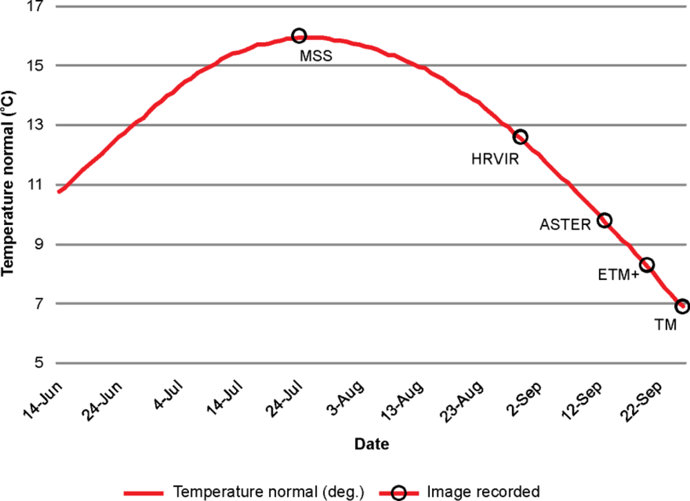
The MSS image was acquired the earliest in the growing season and the TM image, the latest. All five images were acquired at least five weeks after the onset of the growing season as indicated by the date when the sum of degree-days above 0 °C reached 300 °C [32] (Table 2). The sum of degree-days is the highest for the ETM+. However, the NDVI phenology is more favorable for the HRVIR image to yield values higher than those from the TM, ETM+, and ASTER images, which were recorded at later dates in the season when the normal temperatures are below 10 °C (Figure 2).
The MSS image is unique in that it was acquired during the period of summer temperature maxima. The highest seasonal NDVI values are expected about 10 days to two weeks after the peak seasonal temperature had occurred, and then a gradual decrease of the vegetation index follows, consequent with the temperature change [13,67,68]. As a result, the green biomass may not have reached its full potential at the time the MSS image was recorded (see ‘MSS’ on Figure 2); nevertheless it may have been fuller than when the other images were recorded. The seasonal phenology would have caused the MSS derived NDVI values to be higher than those from HRVIR, followed by those from the other three September images.
An evocative approach to assess the NDVI data continuity is by examining temperature anomalies (daily-to-normal temperature difference) on short time periods (of 10 to 40 days) that precede the image acquisition [13]. For all five years, temperature anomalies are of the order of ±1 to 2 °C, over a 40-day period before the image acquisition dates (Table 3). A unique situation among the dataset is that over a 10-day period preceding the HRVIR, the temperature anomaly reached +4.1 °C. The smaller temperature anomalies may have caused NDVI variations of about 5%, most likely positive, for the tree line transition location of the study area, while the large short-term temperature anomaly could have caused a seasonal NDVI fluctuation of up to 10% [13].
5.3. Atmospheric Conditions
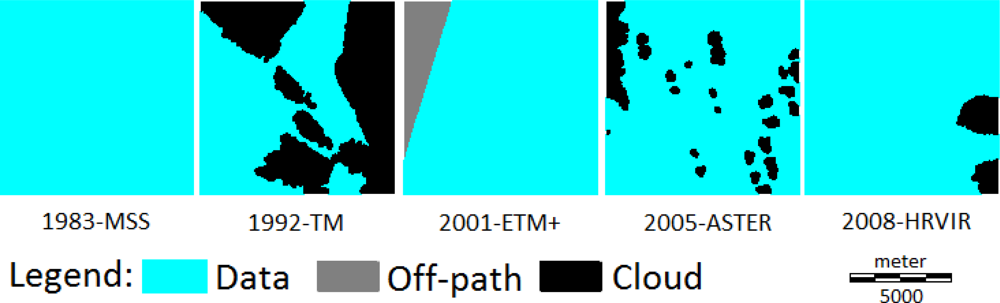
The cloud cover and cloud shadow were identified and masked following the procedure described in Section 6.1.2. The clouds caused 46% and 13% of the study area imaged by TM and ASTER, respectively, to be lost. The MSS and ETM+ are cloud free, while clouds cover only 6% of the HRVIR image (Figure 3). Cumulatively, clouds and their shadows obscure 53% (46% over land, 7% over water) of the study area.
The NDVI values from ASTER may have been more affected than the four other images by atmospheric water vapor absorption in the near-infrared band. The atmospheric humidity recorded from the Goose A weather station [69] at the time the images were acquired range between 33% and 43% for all images, except for the ASTER, which was recorded as the atmospheric humidity reached 73%. The effect of water vapor is to reduce the NDVI value, especially in the higher end of its dynamic range [24].
The across-image NDVI differences due to variations of the atmospheric optical thickness are considered negligible as the weather station reports equal values of visibility during all image acquisitions. However, the visibility that was recorded is 24.1 km, approximately corresponds to an aerosol optical thickness of 0.2 of clear sky [70]. This would have caused the NDVI values above about 0.4 to be underestimated (see Figure 5 in [70]).
6. Image Analysis
The image analysis included preprocessing and extraction of information about the TTI. The preprocessing considered first, a geometric correction that brought all five images to a common reference system, spatial resolution and study area coverage. Second, cloud and water masks were produced, which served as constraint layers for only the cloud-free land portion to be considered in further analyses. Third, atmospheric corrections and cross-sensor calibrations were intended to generate a consistent image dataset.
Information extraction consisted of computing and classifying the NDVI images. Then, the spatial structure of a three-class scheme was examined across the multitemporal dataset. Finally, a linear-form representation of the TTI was derived and its change of position was assessed.
6.1. Preprocessing
6.1.1. Geometric Corrections
An image-to-image geometric correction of the 1983, 1992, 2005 and 2008 data to the 2001- ETM+ orthoimage (UTM Zone 21-North and North American Datum (NAD) 1983) took the multitemporal set to a 30 m pixel size, which complies with the current remote sensing image analysis protocol for mapping Canada’s arctic vegetation [1].
The TM, ASTER and HRVIR images’ initial spatial resolutions are the same or finer than that of the reference ETM+ image (Table 1). The nearest neighbour interpolation was applied for those images with which the ground control points could be located based on visual interpretation of similar brightness values in corresponding spectral bands. However, the MSS image spatial resolution was much coarser than that of the output matrix. In order to produce a gradual transition from the input to the output resolution, the path-projected MSS pixels were expanded upon by a factor of four in row and column directions, to a 20 m pixel size, and the bilinear interpolation resampling function was applied. The pixel replication facilitated the relative location (i.e., ‘middle’ or ‘edges’) of ground control points within the same-brightness values areas corresponding to the initial 80 m image units.
The number of ground control points for each image is 16 for the 1992, 2005 and 2008 images and 12 for the 1983 image. GCPs included small islands and lake shorelines with unique profiles, as anthropogenic features such as road intersections, were not present in any of the images. The GCPs were uniformly selected throughout each image. Each resulting geo-corrected image has a total root-mean-square error equivalent to less than a half of their initial spatial resolution (37, 15, 3, and 7 m for MSS, TM, ASTER and HRVIR, respectively).
6.1.2. Cloud, Cloud Shadow, and Water Masks
The 1983 MSS image served as the cloud-free image standard for the discrimination of clouds and cloud shadows on the 1992, 2005 and 2008 images. The image ratio change detection analysis [71,72] consisted of applying a two-date red spectral band image ratio of the cloud-free image to the cloud-affected image. The overlay operation enhanced the clouds and their shadow. On the cloud-enhanced image histogram, the lowest and highest values characterize the cloud shadows and clouds, respectively. Once classified, these areas were expanded upon with a five-pixel buffer. This buffer width was chosen because it included thinner clouds that were identified by visual inspection of the images, but that had not been included in the automatically classified clouds category.
NDVI images are relevant only to the land portion of the image, therefore justifying the application of a water mask. The near-infrared band bimodal histogram, which displays distinctive distributions for water and land [73], is classified with reference to the threshold reflectance value that recorded the lowest histogram frequency between the water and land values.
The clouds, cloud shadows and water mask were integrated through image overlay to each image of the set and, separately, a cumulative ‘no data’ mask was applied to the images.
6.1.3. Atmospheric Corrections and Radiometric Cross-Calibrations
Continuity of NDVI values ideally relies on sensor pairwise cross-calibration of the individual bands reflectance values, which may vary in relation to the land cover [25,65]. The radiometric preprocessing included, first, a calibration of the individual images and spectral bands to the ‘at-satellite apparent reflectance’ value, with the integration of a Rayleigh scattering path radiance equivalent (i.e., dark-pixel subtraction) correction. Second, a multitemporal cross-calibration adjusted the reflectance values of corresponding spectral bands across the five images. Both calibrations methods were used in order to minimize the potential errors due, on the one hand, to atmospheric moisture conditions that affected the images and that would not have been all accounted for in a path radiance equivalent correction, and on the other hand, the difficulty to find a calibration points (same land cover) in images that were collected over a period of 25 years and varying cloud covers.
The radiance calibration values for the three Landsat images were documented by [26] while the HRVIR parameters were contained in the image metadata. No calibration parameters accompanied the ASTER image, therefore, in this case, the individual spectral band calibration was omitted and the raw image was input to the cross-calibration. The individual spectral band calibration incorporated atmospheric corrections based on the dark object subtraction method to minimize the effect of Rayleigh scattering [74]. The image histogram non-zero minimum brightness values (BV) provided the haze equivalent estimates.
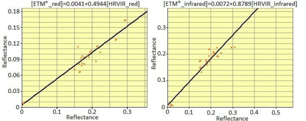
The multitemporal relative correction, or cross-calibration, aimed to normalize to a reference image, the at-satellite apparent reflectance of its corresponding spectral band. The 2001-ETM+ image served as the reference image due to the cloud-free conditions during which it was acquired. In addition, the ETM+ red and near-infrared passbands are best matched to the corresponding bands of the other images in the dataset. The calibration is based on regression equations obtained from 31 points, each chosen to represent a pseudo-invariant feature (PIF) [75] throughout the study area. PIFs for this particular area included barren surfaces and deep water bodies, as these features are shown to have little variation in spectral reflectance across the multitemporal dataset. The spectral characteristics of a PIF must be consistent between the reference image and the image being calibrated. An example of the linear regression graph between the ETM+ image and the SPOT image is presented in Figure 4.
A linear regression of the 2001 and each of the other four image sets is calculated from the PIFs, from which the cross-calibration equations are derived. For each, the independent variable of the regression is the image to be calibrated. The dependent variable is the 2001 corresponding spectral band. The regression equation (Equation (2)), y-intercept (A0) and slope (A1) provide the necessary information to compute from each multitemporal image (INPyear) a calibrated image that highly correlates with the 2001 reference image (CALyear). Table 4 reports the cross-calibration equation parameters and coefficient of determination values.
6.2. Information Extraction
6.2.1. Vegetation Index Image Calculation, Classification, and Validation
The NDVI computed from the near-infrared and red calibrated images of each year (Equation (1)), provided a representation of the green vegetation cover distribution. A red reflectance decrease and an infrared reflectance increase translate into an increased NDVI.
The NDVI images were classified into ordinal categories that represented the vegetation cover while incorporating the anomalies identified to the sensors’ spectrometry, atmospheric conditions and to the vegetation phenology throughout the multitemporal dataset. The areas for which data are cumulatively available on all five images (cloud-, cloud shadow-free and in-image path) were used to set the NDVI classification boundaries. The positive NDVI values were grouped into three categories based on quartile distributions. The interquartile values (middle 50%) of each year-distribution were grouped in the class ‘intermediate’. The values included in the lowest and highest quartile ranges were assigned to the ‘low’ and ‘high’ NDVI classes, respectively.
The ecological significance of the NDVI classes was evaluated using the Fisher’s exact probability test [76]. The null hypothesis is of no difference in the ‘low’ and ‘high’ NDVI categories considering the field data representing ‘tundra’ and ‘taiga’ land cover types as defined in Section 3 for which field data were available.
6.2.2. NDVI Spatial Distribution and Within Class Variation
Information about the horizontal distribution of the TTI was extracted by overlay of the five image set to identify the areas that are, on at least four of the five images, repeatedly in one of the three NDVI classes. This analysis caused patterns of consistent low, intermediate and high vegetation indices to emerge.
The within-class median NDVI value for each of the three consistent NDVI categories was computed. The results of this analysis are represented and put in context of the errors that were attributed to spectral resolution and short-term temperature anomalies.
6.2.3. Estimating the Location of the Tree Line
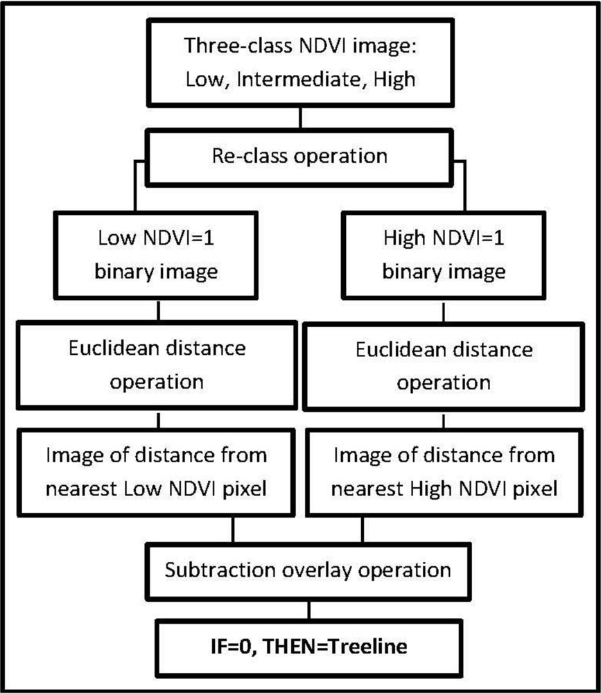
Tentatively, the intermediate NDVI class represents a transition class between the taiga and the tundra land cover classes. This class is expressed as the TTI, i.e., where the tundra and taiga environment interact. The transition from taiga to tundra is gradual because it occurs along a sizable distance that forms a corridor-shaped area. The TTI, as represented by the intermediate NDVI class, cannot be monitored based on the information that we have extracted and interpreted from the dataset because it is spatially fragmented (Table 5). For example, the maximum area size for continuous intermediate NDVI patches is 7 ha, with a median size of 1 ha which correspond to only a few TM or MSS pixels. In addition, the field data were collection protocol focused land cover description within 30 × 30 m2 sampling areas. Therefore, it is practical to further this study by estimating a ‘tree line’ halfway between the low NDVI and high NDVI classes which were validated using field data collected for tundra and taiga land cover types, respectively. This tree line was estimated to help assess the magnitude of changes.
The tree line estimation process flowchart is presented on Figure 5. The area perimeter of low and high NDVI served as anchor to calculate the radiating Euclidean distance and to automatically identify the pixels that are halfway between them, at which location an ‘estimated’ tree line is drawn. The halfway distance was identified by subtraction overlay where the output image value of zero was assigned to pixels situated where the distance calculated from the low NDVI is equal to the distance from the high NDVI.
Then, contingency analyses of the 1983-2001-2008 and the 2001-2005-2008 image sets brought out long- and short-term changes, respectively. The tree line was estimated on each image without considering the water, cloud and cloud shadow categories. The 1992 image was excluded from this analysis because of the impeding cloud cover.
With each image set, the distance was automatically calculated from the tree line on the earliest image date (1983 or 2001) to the displaced tree line segments on the second and third images (2001 and 2008, or 2005 and 2008). The displacement distances were calculated by overlay of the estimated tree line-migrated segment image and a distance gradient from the earliest date’s estimated tree line image.
7. Results
Table 6 presents the descriptive statistics of the five NDVI images. Relatively low mean and maximum NDVI values emerged from the 1983 MSS and the 1992 TM data. The NDVI values calculated from the 2008 HRVIR image are the highest, with an average value of 0.60. It is about 0.05 to 0.20 higher than that of the average NDVI computed from the other images.
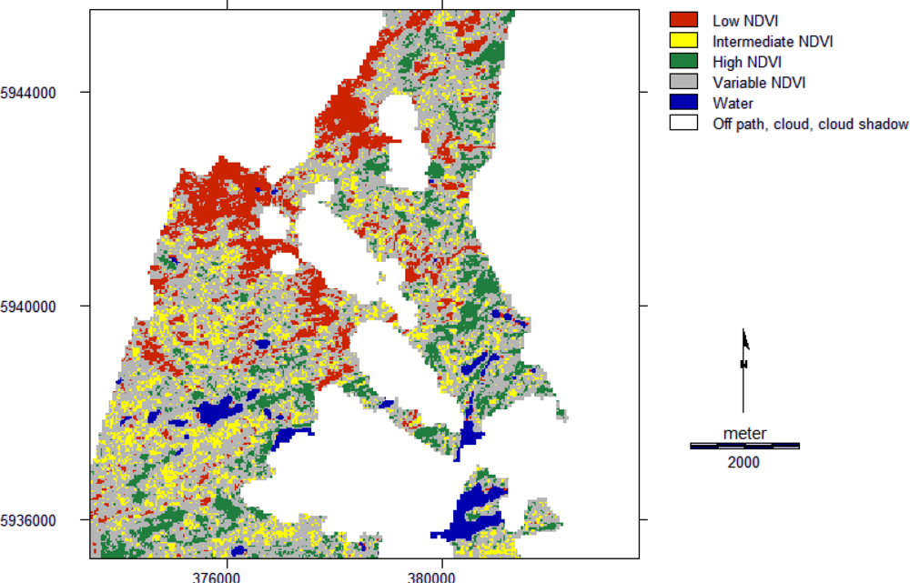
The quartile distribution-based NDVI classes are listed in Table 7 and the most consistently classified areas are displayed on Figure 6; a consistent area is where same one of the three NDVI class is present on at least four of the five images. Areas where the low and high NDVI remained similar over the 25-year period have the largest and most variable unit sizes (Table 5). Conversely, the intermediate NDVI category is highly fragmented into parcels that are of the order of 1 to 3 ha in size.
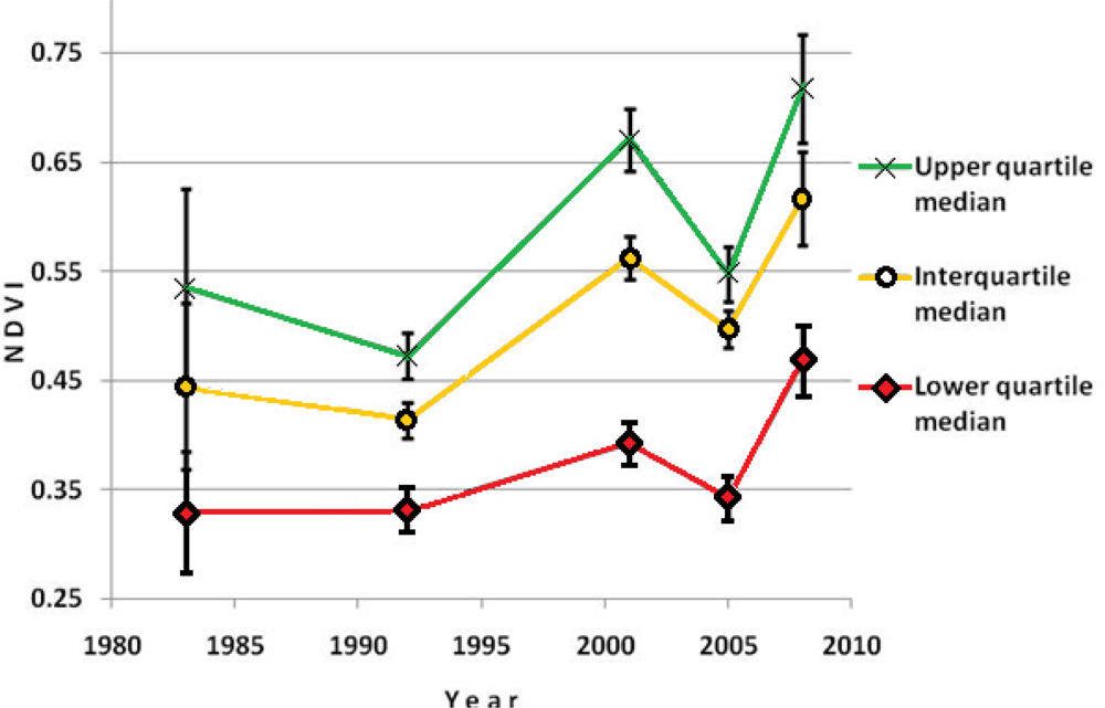
The within-class median NDVI value computed for each of the three consistent NDVI categories show an increasing trend from 1983 to 2008 (Figure 7). During this period, the median values for the low, intermediate and high NDVI classes increased by 42%, 39%, and 34%, respectively. These changes are robust to the estimated errors due to a wider passband on the 1983 image (7%) and short-term temperature anomalies (5% for all images and 10% for the 2008 image).
Table 8 presents the contingency tables and the Fisher’s exact test results. The null hypothesis was rejected for all five images, meaning a significant association (α = 0.05) between the classes that describe the lowest and highest NDVI values and the field-observed vegetation cover. Given the NDVI values involved that were documented in the literature (see Section 4) [6,35,40,61,62] and the Fisher’s test results, the low, intermediate, and high NDVI classes were matched with the tundra, TTI, and taiga land cover types, respectively.
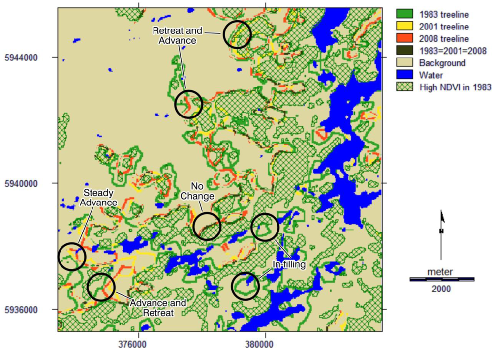
The multitemporal image on Figure 8 illustrates the 1983 to 2008 changes. Lines of different colours represent the tree line location at different dates and the black line indicates that no change occurred over the period of observation. For visual reference, the green-gridded feature in the southeast portion of the image is the area of high NDVI for 1983, which is the initial date of the three- image series.
Segments of a few kilometers in length of the estimated tree line keep a steady position with changes that do not exceed 90 m over the period of observation. At other locations it is unstable as it alternatively records advances and retreats, as well as displaying steady advances or retreats. At locations in the southeast portion, in the low lands of the study area, the estimated tree line makes advances of the order of 200 to 300 m when comparing the 1983 and the 2008 images. Also in this area, the estimated 1983-tree line showed several discontinuities (evidenced by a multitude of circling tree line segments) that were filled-in as represented on the 2001 and 2008 images.
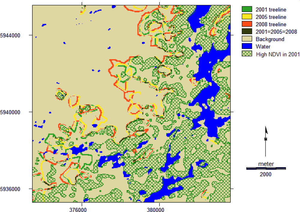
The multitemporal image on Figure 9 illustrates the 2001 to 2008 changes. It is constructed and interpreted in the same manner as Figure 8 except for that the green gridded area represents the 2001 high NDVI class. As observed on the long-term multitemporal image, segments of few kilometers of the estimated tree line have remained stable between 2001 and 2008. In the center area of the image, noticeable advances from high to low NDVI are recorded, especially for the last portion of the time series, between 2005 and 2008.
Table 9 reports an overall advance-to-retreat net difference of no more than the equivalent of one pixel (30 m) in the position of tree line segments for the two long-term image sequences. During the shorter period of observation that follows, from 2001 to 2008, a 60 m change is recorded. The highest estimated tree line migration distances correspond with an advance.
Changes of the tree line estimated at halfway between the low and high NDVI classes, indicate a net progression of 10 to 60 m over the different periods of time. Locally, the variations are much larger than the image’s spatial resolution. The tree line segments that are subject to gradual migration or retreat depart by up to 320 m from the estimated position of the 1983 or 2001 tree line. The most stable portions of the tree line, which have not shown change of more than 90 m, are of the order of 3 to 4 km in length (Figures 8 and 9).
The clouds are not shown on the composite images because the tree line location is estimated from the low and high NDVI class patches, through this process any other class would not be considered. The 1983 image is cloud free, as well as the 1992 image. The clouds on the 2008 image do not interfere because they are in the southeast corner of the study area (Figure 3) and away from the transition zone. Small clouds may have affected the 2005 estimated tree line on the short-term change image by spatially interrupting the distribution and producing smaller patches of low and high NDVI from which the tree line was calculated.
8. Discussion
Changes in green biomass, represented through the NDVI, and its spatial distribution were mapped from a multitemporal image series acquired by five different sensors. The analysis resulted with ordinal NDVI categories that incorporate the variations due to acquisition asynchrony caused by the seasonal temperature anomalies and cross-sensor spectral inconsistencies. The quartile-based NDVI classes are representative of land covers found near the tundra-taiga interface. Throughout the 25-year period of observation, all three classes display an increase of the trend in NDVI values. These are of the order of 40%. In addition, an estimated tree line was derived, which allowed to illustrate and quantify long- and short-term changes in the landscape.
Some of the sources of NDVI anomalies reviewed in Section 5 may have affected the dataset. In particular, lower NDVI values in the 1983 image may be attributed to the different infrared passband on the MSS sensor. The TM-derived NDVI image displays the smallest coefficient of variation as well as the lowest average value. These may have been caused by a lower level of incident radiation due to extensive cloud coverage during the 1992 image acquisition. Yet, the low and high NDVI categories were tied with the field-recorded land cover descriptions.
The highest NDVI values calculated from the 2008 HRVIR may have been caused by the short-term temperature anomalies prior to the image acquisition date. Nevertheless, the phenological state at the time of the MSS image was recorded, one month earlier in mid-July, also works in favor of a greener land cover. This might explain on the long-term change image that some portions of the estimated tree line have receded.
An important issue of multitemporal image analysis is that the validation of historical images, which are these images that were recorded before one engages in a monitoring study, have no coincident field data or very little if fortuitously it was collected for other purposes. The Fisher’s test results reported in Table 8 are all significant and there is no apparent unbalance of the distribution of the observations in the contingency tables for the different images, including that of coincident HRVIR image. This is an indication that the field data were collected in area where no important change had occurred. In addition, the contingency tables reveal a mix of tundra and taiga field observations in the intermediate NDVI category; because of this it is anticipated that this class gives a correct representation of the TTI on the image. Noticeably, this area contains a larger proportion of tundra samples in 1983 (14 of 22 observations, or 64%) and 1992 (61%), while a more even representation of tundra and taiga field records are found in the intermediate NDVI class on the 2001, 2005 and 2008 images.
The categories of low and high NDVI occur in patches that have dimensions that are much larger than the dataset’s coarsest resolution (that of MSS with 80 × 80 m2 or 0.64 ha pixel size). Also, more than half the parcels forming the transition zone (intermediate NDVI class) have sizes of about 1 ha. Therefore, as expected, the MSS spatial resolution is inappropriate for monitoring the progression of features such as tree islands and encroachments that are found at the boundary and within the TTI. For this purpose, neither is appropriate the TM image 30 m resolution, with about 11 pixels per ha.
The image analysis revealed increase of the TTI density. The 1983-to-2008 change image (Figure 8) indicates in-filling of areas that were not in the high NDVI class in 1983. The in-filled areas are shown by the 1983-line (green) forming closed loops that are not duplicated by the other tree lines (yellow and red). These patterns take place on the long-term change image only. A similar dynamics, whereby changes occurred from sparse to open, and from open to normal stand was reported by [32] for the period of 1980 to 2000 in forest-tundra larch forests Ary-Mas, Russia.
The investigation of the TTI as an area feature that corresponds to the intermediate NDVI category must be based on spatial and temporal resolution images that have not been available until just recently. Given the 1 ha area formed by intermediate NDVI patches, and considering a 3 × 3 pixel array for being able to observe a 1-pixel migration, 30 m is the coarsest spatial resolution appropriate for detecting variations within the transition area. In light of this evaluation, the spatial resolution prescribed in the protocol for mapping Canada’s arctic vegetation [1] may have to be reconsidered when focusing on regional scale observations of the tundra-taiga interface.
An uneven advance of the tree line is observed from the result of this study. While several segments may not have changed at all over the years, some portions have retreated and others display 270 m (68 m per year from 2001 to 2005) to 320 m (46 m per year from 2001 to 2008) horizontal progression in the direction of the tundra. These values are lower than the rates of 0.2 to 0.4 km per year stated by [48] for Eastern Canada.
The difference between the advance and retreat median values concludes to a net advance of 9 m per year, for the period from 2001 to 2008 (Table 9: 150 m advance less 90 m retreat over a 7 year period). This is consistent with the advances of 3 to 11 m per year for the period of 1980–2000 in northern Russia [32], but it is much lower than the mean advance of 378 m per year (2.5 km from 2000 to 2009) reported for the pine forest line in northern Norway [77]. The variations observed for the Mealy Mountains study are attributed to site conditions, as seedling in the TTI in Labrador can be affected by the soil wetness, wind exposure, temperature [78], seedbed composition [79] and the topography [80]. The impact of these factors, individually or in combination, yet has to be investigated in relation to the information that was extracted from the satellite images.
The revisit frequency of visible and near-infrared image systems is in effect reduced due to cloud cover and atmospheric moisture degraded signal. Such issues prevent the acquisition of high temporal resolution image series that would allow for characterization of the vegetation’s annual phenology and to differentiate this from long-term changes. The prospect of using radar image-based vegetation mapping [39,81] circumvents this issue by potentially increasing the temporal resolution, while spatial resolutions available are finer than the 30 m used in this study. Further work must investigate the information that can be extracted from radar images, which is not dependent on the vegetation’s photosynthetic activity, as the NDVI is, but on the spatial structure of the components of the tundra and taiga environments and of the transition zone separating them.
9. Conclusion
This paper presents evidence that the green biomass, represented by the Normalized Difference Vegetation Index (NDVI), has increased between 1983 and 2008, and more importantly between 2001 and 2008, in a portion of the Canadian tundra-taiga interface (TTI). The results of this study are based on the analysis of a multisensor NDVI image series that had been recorded using different spectral and spatial resolutions, and under variable atmospheric conditions. A cross-sensor calibration and the classification of the vegetation index in ordinal classes produced a consistent dataset from which a NDVI-inferred biomass overall increasing trend of about 40% was detected. The change in biomass is more accentuated for the low NDVI than for the high NDVI category, which rendered an increasing trend of 42% and 34%, respectively.
Spatially, a migration of the taiga environment, represented by high NDVI values, toward the tundra occurred. This observation emerged from changes in the location of a tree line derived from the classified images. Overall, no significant difference was detected between the tree line estimated from the 1983 and the 2008 images, while a net advance of 60 m, or 9 m per year, was observed between 2001 and 2008. Horizontal migrations of 130 to 320 m were recorded for short segments of the estimated tree line during the various periods of observations.
In characterizing of the TTI as an area, rather than as a linear feature, the research highlighted that it has a large spatial variability, represented by the patch size, of the low and high NDVI classes. Consequently, the monitoring of the TTI would preferably rely on image spatial resolutions of 20 m (25 pixels per ha) or finer.
A multisensor image set can successfully be used to monitor the TTI and potentially expand to include the latest medium to high spatial resolution multispectral images such as acquired from the Landsat-8, QuickBird, and WorldView-2 platforms. As well, further work for the study area of the Mealy Mountains, Labrador, addresses the transition from multispectral to radar image for monitoring the tundra-taiga interface.
Acknowledgments
We acknowledge funding from the Government of Canada Program for International Polar Year as part of the project Present processes, Past changes, Spatiotemporal dynamics (PPS) Arctic Canada (Karen Harper, Alvin Simms). This project is a product under the IPY core project PPS Arctic as part of the International Polar Year 2007–2008, which was sponsored by the International Council for Science and the World Meteorological Organisation. This funding contributed to graduate student support, the purchase of satellite images and image analysis software licenses. The authors would like to thank the anonymous referees for their helpful constructive suggestions.
References
- Chen, W. IPY CiCAT Field Measurement Protocol for Mapping Canada’s Arctic Vegetation, Version 4.0; Natural Resources: Ottawa, ON, Canada, 2007. [Google Scholar]
- Walker, D.A.; Auerbach, N.A.; Shippert, M.M. NDVI, biomass, and landscape evolution of glaciated terrain in northern Alaska. Polar Rec 1995, 31, 169–178. [Google Scholar]
- Kelley, A.M.; Epstein, H.E.; Walker, D.A. Role of vegetation and climate in permafrost active layer depth in Arctic tundra of Northern Alaska and Canada. J. Glaciol. Geocryol 2004, 26, 269–274. [Google Scholar]
- Raynolds, M.K.; Walker, D.A.; Maier, H.A. NDVI patterns and phytomass distribution in the circumpolar Arctic. Remote Sens. Env 2006, 102, 271–281. [Google Scholar]
- Engstrom, R.; Hope, A.; Kwon, H.; Stow, D. The relationship between soil moisture and NDVI near Barrow, Alaska. Phys. Geog 2008, 29, 38–53. [Google Scholar]
- Munger, C.A.; Walker, D.A.; Maier, H.A.; Hamilton, T.D. Spatial Analysis of Glacial Geology, Surficial Geomorphology, and Vegetation in the Toolik Lake Region: Relevance to Past and Future Land-Cover Changes. Proceedings of the Ninth International Conference on Permafrost, Fairbanks, AK, USA, 28 June–3 July 2008; pp. 1255–1260.
- Van Wijk, M.T.; Williams, M. Optical instruments for measuring leaf area index in low vegetation: application in Arctic ecosystems. Ecol. Appl 2005, 15, 1462–1470. [Google Scholar]
- Blok, D.; Schaepman-Strub, G.; Bartholomeus, H.; Heijmans, M.M.P.D.; Maximov, T.C.; Berendse, F. The response of Arctic vegetation to the summer climate: relation between shrub cover, NDVI, surface albedo and temperature. Environ. Res. Lett 2011, 6, 035502. [Google Scholar]
- Stow, D.; Hope, A.; Boyton, W.; Phinn, S.; Walker, D.; Auerbach, N. Satellite-derived vegetation index and cover type maps for estimating carbon dioxide flux for Arctic tundra regions. Geomorphology 1998, 21, 313–327. [Google Scholar]
- Walker, D.A.; Epstein, H.E.; Jia, G.J.; Balser, A.; Copass, C.; Edwards, E.J.; Gould, W.A.; Hollingsworth, J.; Knudson, J.; Maier, H.A.; et al. Phytomass, LAI, and NDVI in northern Alaska: Relationships to summer warmth, soil pH, plant functional types and extrapolation to the circumpolar Arctic. J. Geophys. Res 2003, 108, 8169. [Google Scholar]
- Hope, A.S.; Pence, K.R.; Stow, D.A. NDVI from low altitude aircraft and composited NOAA AVHRR data for scaling Arctic ecosystem fluxes. Int. J. Remote Sens 2004, 25, 4237–4250. [Google Scholar]
- Wang, M.; Overland, J.E. Detecting Arctic climate change using Koppen climate classification. Climatic Change 2004, 67, 43–62. [Google Scholar]
- Olthof, I.; Latifovic, R. Short-term response of Arctic vegetation NDVI to temperature anomalies. Int. J. Remote Sens 2007, 28, 4823–4840. [Google Scholar]
- Raynolds, M.K.; Comiso, J.C.; Walker, D.A.; Verbyla, D. Relationship between satellite-derived land surface temperatures, Arctic vegetation types, and NDVI. Remote Sens. Environ 2008, 112, 1884–1894. [Google Scholar]
- Zhang, K.; Kimball, J.S.; Mu, Q.; Jones, L.A.; Goetz, S.J.; Running, S.W. Satellite based analysis of northern ET trends and associated changes in the regional water balance from 1983 to 2005. J. Hydrol 2008, 379, 92–110. [Google Scholar]
- Hansen, M.C.; DeFries, R.S.; Townshend, J.R.; Carroll, G.M.; Dimiceli, C.; Sohlberg, R.A. Global percent tree cover at a spatial resolution of 500 meters: First results of the MODIS vegetation continuous fields algorithm. Earth Interact 2003, 7, 1–15. [Google Scholar]
- Yoshioka, H.; Miura, T.; Huete, A.R. An isoline-based translation technique of spectral vegetation index using EO-1 Hyperion data. IEEE Trans. Geosci. Remote 2003, 41, 1363–1372. [Google Scholar]
- Olthof, I.; Pouliot, D.; Fernandes, R.; Latifovic, R. Landsat-7 ETM+ radiometric normalization comparison for northern mapping applications. Remote Sens. Environ 2005, 95, 388–398. [Google Scholar]
- Brown, M.E.; Pinzón, J.E.; Didan, K.; Morisette, J.T.; Tucker, C.J. Evaluation of the consistency of long-term NDVI time series derived from AVHRR, SPOT-Vegetation, SeaWiFS, MODIS, and Landsat ETM+ sensors. IEEE Trans. Geosci. Remote 2006, 44, 1787–1793. [Google Scholar]
- Stow, D.; Petersen, A.; Hope, A.; Engstrom, R.; Coulter, L. Greenness trends of Arctic tundra vegetation in the 1990s: Comparison of two NDVI data sets from NOAA AVHRR systems. Int. J. Remote Sens 2007, 28, 4807–4822. [Google Scholar]
- Stow, D.; Daeschner, S.; Boyton, W.; Hope, A. Arctic tundra functional types by classification of single-date and AVHRR bi-weekly NDVI composite datasets. Int. J. Remote Sens 2000, 21, 1773–1779. [Google Scholar]
- Laidler, G.J.; Treitz, P.M.; Atkinson, D.M. Remote sensing of arctic vegetation: Relations between the NDVI, spatial resolution and vegetation cover on Boothia Peninsula, Nunavut. Arctic 2008, 61, 1–13. [Google Scholar]
- Olthof, I.; Pouliot, D. Treeline vegetation composition and change in Canada’s western Subarctic from AVHRR and canopy reflectance modeling. Remote Sens. Environ 2010, 114, 805–815. [Google Scholar]
- Van Leeuwen, W.J.D.; Orr, B.J.; Marsh, S.E.; Herrmann, S.M. Multi-sensor NDVI data continuity: Uncertainties and implications for vegetation monitoring applications. Remote Sens. Environ 2006, 100, 67–81. [Google Scholar]
- Teillet, P.M.; Fedosejevs, G.; Thome, K.J.; Barker, J.L. Impacts of spectral band difference effects on radiometric cross-calibration between satellite sensors in the solar-reflective spectral domain. Remote Sens. Environ 2007, 110, 393–409. [Google Scholar]
- Chander, G.; Markham, B.L.; Helder, D.L. Summary of current radiometric calibration coefficients for Landsat MSS, TM, ETM+, and EO-1 ALI sensors. Remote Sens. Environ 2009, 113, 893–903. [Google Scholar]
- Jordan, C.F. Derivation of leaf area index from quality of light on the forest floor. Ecology 1969, 50, 663–666. [Google Scholar]
- Hope, A.S.; Engstrom, R.; Stow, D. Relationship between AVHRR surface temperature and NDVI in Arctic tundra ecosystems. Int. J. Remote Sens 2004, 26, 1771–1776. [Google Scholar]
- Narasimhan, R.; Stow, D. Daily MODIS products for analyzing early season vegetation dynamics across the North Slope of Alaska. Remote Sens. Environ 2010, 114, 1251–1262. [Google Scholar]
- Pouliot, D.; Latifovic, R.; Olthof, I. Trend in vegetation NDVI from 1 km AVHRR data over Canada for the period 1985–2006. Int. J. Remote Sens 2009, 30, 149–168. [Google Scholar]
- Scott, P.A.; Hansell, R.I.C. Development of white spruce tree islands in the shrub zone of the forest-tundra. Arctic 2000, 55, 238–246. [Google Scholar]
- Kharuk, V.I.; Ranson, K.J.; Im, S.T.; Naurzabaev, M.M. Forest-tundra larch forests and climatic trends. Russ. J. Ecol 2006, 37, 291–298. [Google Scholar]
- Rees, W.G. Characterisation of Arctic treelines by LiDAR and multispectral imagery. Polar Rec 2007, 43, 345–352. [Google Scholar]
- Shippert, M.; Walker, D.A.; Auerbach, N.A. Biomass and leaf area index maps derived from SPOT images for Toolik Lake and Imnavait Creek area, Alaska. Polar Rec 1995, 31, 147–154. [Google Scholar]
- Riedel, S.M.; Epstein, H.E.; Walker, D.A. Biotic controls over spectral reflectance of Arctic tundra vegetation. Int. J. Remote Sens 2005, 26, 2391–2405. [Google Scholar]
- Regmi, P.; Grosse, G.; Jones, M.C.; Jones, B.M.; Anthony, K.W. Characterizing post-drainage succession in thermokarst lake basins on the Seward Peninsula, Alaska with TerraSAR-X backscatter and Landsat-based NDVI data. Remote Sens 2012, 4, 3741–3765. [Google Scholar]
- Atkinson, D.M.; Treitz, P. Arctic ecological classifications derived from vegetation community and satellite spectral data. Remote Sens 2012, 4, 3948–3971. [Google Scholar]
- Bubier, J.L.; Rock, B.N.; Crill, P.M. Spectral reflectance measurements of boreal wetland and forest mosses. J. Geophys. Res 1997, 102, 29489–29494. [Google Scholar]
- Ranson, K.J.; Sun, G.; Kharuk, V.I.; Kovacs, K. Assessing tundra-taiga boundary with multi-sensor satellite data. Remote Sens. Environ 2004, 93, 283–295. [Google Scholar]
- Chen, X.; Vierling, L.; Deering, D. A simple and effective radiometric correction method to improve landscape change detection across sensors and across time. Remote Sens. Environ 2005, 98, 63–79. [Google Scholar]
- Kumpula, T.; Forbes, B.C.; Stammler, F.; Meschtyb, N. Dynamics of a coupled system: Multi-Resolution remote sensing in assessing social-ecological responses during 25 years of gas field development in Arctic Russia. Remote Sens 2012, 4, 1046–1068. [Google Scholar]
- Zhang, Y.; Xu, M.; Adams, J.; Wang, X. Can Landsat imagery detect tree line dynamics? Int. J. Remote Sens 2009, 30, 1327–1340. [Google Scholar]
- Batterson, M.; Liverman, D. Landscapes of Newfoundland and Labrador Report 95–3; Newfoundland and Labrador-Department of Natural Resources: St. John’s, NL, Canada, 1995. [Google Scholar]
- Clark, C.D.; Knight, J.K.; Gray, J.T. Geomorphological reconstruction of the Labrador sector of the Laurentide Ice Sheet. Quaternary Sci. Rev 2000, 19, 1343–1366. [Google Scholar]
- Roberts, B.A.; Simon, N.P.P.; Deering, K.W. The forests and woodlands of Labrador, Canada: ecology, distribution and future management. Ecol. Res 2006, 21, 868–880. [Google Scholar]
- Ryan, A.G. Native Trees and Shrubs of Newfoundland and Labrador; Department of Environment and Lands: St. John’s, NL, Canada, 1978. [Google Scholar]
- Munier, A. Seedling Establishment and Climate Change: The Potential for Forest Displacement of Alpine Tundra (Mealy Mountains, Labrador, Canada). M.Sc. Thesis, Memorial University, St. John’s, NL, Canada, 2006.
- Callaghan, T.V.; Crawford, R.M.M.; Eronen, M.; Hofgaard, A.; Payette, S.; Rees, W.G.; Skre, O.; Sveinbjörnsson, B.; Vlassova, T.K.; Werkman, B.R. The dynamics of the tundra-taiga boundary: An overview and suggested coordinated and integrated approach to research. Ambio 2002, 12, 2–5. [Google Scholar]
- Skre, O.; Baxter, R.; Crawford, R.M.M.; Callaghan, T.V.; Fedorkov, A. How will the tundra-taiga interface respond to climate change? Ambio 2002, 8, 37–46. [Google Scholar]
- Hermanutz, L. Personal Webpage; Memorial University: St. John’s, NL, Canada, 2011. Available online: http://www.mun.ca/biology/lhermanutz/lhermanutz.php (accessed on 10 December 2012).
- Tucker, C.J. Red and photographic infrared linear combinations for monitoring vegetation. Remote Sens. Environ 1979, 8, 127–150. [Google Scholar]
- Rouse, J.W., Jr.; Haas, R.H.; Schell, J.A.; Deering, D.W. Monitoring Vegetation Systems in the Great Plains with ERTS. Proceedings of NASA. Goddard Space Flight Center 3nd ERTS-1 Symposium, Greenbelt, MD, USA, 5–9 March 1974; 1, pp. 309–317.
- Natural Resources Canada. Canada Centre for Remote Sensing Earth Observation Catalogue—CEOcat, Available online: http://ceocat.ccrs.nrcan.gc.ca/portal/index.html (accessed on 10 December 2012).
- United States Geological Survey. Earth Explorer, Available online: http://earthexplorer.usgs.gov (accessed on 10 December 2012).
- Jet Propulsion Laboratory-National Aeronautics and Space Administration. Advanced Space Thermal Emission and Reflection Radiometer Instrument Characteristics; Available online: asterweb.jpl.nasa.gov/characteristics.asp (accessed on 10 December 2012).
- Belgian Science Policy. Satellites and Sensors: Satellite Pour l’Observation de la Terre, Available online: http://eoedu.belspo.be/en/satellites/index.htm (accessed on 10 December 2012).
- Hall, F.G.; Shimabukuro, Y.E.; Huemmrich, K.F. Remote sensing of forest biophysical structure using mixture decomposition and geometric reflectance models. Ecol. Appl 1995, 5, 993–1013. [Google Scholar]
- Sturm, M.; Racine, C.; Tape, K. Increasing shrub abundance in the Arctic. Nature 2001, 411, 546–547. [Google Scholar]
- Nakaji, T.; Oguma, H.; Fujinuma, Y. Seasonal changes in the relationship between photochemical reflectance index and photosynthetic light use efficiency of Japanese larch needles. Int. J. Remote Sens 2006, 27, 493–509. [Google Scholar]
- Kobayashi, H.; Suzuki, R.; Kobayashi, S. Reflectance seasonality and its relation to the canopy leaf area index in an eastern Siberian larch forest: Multi-satellite data and radiative transfer analyses. Remote Sens. Environ 2007, 106, 238–252. [Google Scholar]
- Hope, A.S.; Kimball, J.S.; Stow, D.A. The relationship between tussock tundra spectral reflectance properties and biomass and vegetation composition. Int. J. Remote Sens 1993, 14, 1861–1874. [Google Scholar]
- Jia, G.J.; Epstein, H.E.; Walker, D.A. Spatial heterogeneity of tundra vegetation response to recent temperature changes. Global Change Biol. 2006, 12, 42–55. [Google Scholar]
- Vogelmann, J.E.; Moss, D.M. Spectral reflectance measurements in the Genus ‘Sphagnum’. Remote Sens. Environ 1993, 45, 273–279. [Google Scholar]
- Rees, W.G.; Tutubalina, O.V.; Golubeva, E.I. Reflectance spectra of Subarctic lichens between 400 and 2400 nm. Remote Sens. Environ 2004, 90, 281–292. [Google Scholar]
- Miura, T.; Huete, A.; Yoshioka, H. An empirical investigation of cross-sensor relationships of NDVI and red/near-infrared reflectance using EO-1 Hyperion data. Remote Sens. Environ 2006, 100, 223–236. [Google Scholar]
- Steven, M.D.; Malthus, T.J.; Baret, F.; Xu, H.; Chopping, M.J. Intercalibration of vegetation indices from different sensor systems. Remote Sens. Environ 2003, 88, 412–422. [Google Scholar]
- Tutubalina, O.V.; Rees, W.G. Vegetation degradation in a permafrost region as seen from space: Noril'sk, 1961–1999. Cold Reg. Sci. Technol 2001, 32, 191–203. [Google Scholar]
- Forbes, B.C.; Fauria, M.M.; Zetterberg, P. Russian Arctic warming and ‘greening’ are closely tracked by tundra shrub willows. Global Change Biol 2010, 16, 1542–1554. [Google Scholar]
- Environment Canada-National Climate Data and Information Archive. Hourly Data Report, Available online: http://www.climate.weatheroffice.gc.ca/climateData/canada_e.html (accessed on 10 December 2012).
- Kaufman, Y.J.; Tanré, D. Strategy for direct and indirect methods for correcting the aerosol effect on remote sensing: From AVHRR to EOS-MODIS. Remote Sens. Environ 1996, 55, 65–79. [Google Scholar]
- Sing, A. Digital change detection techniques using remotely-sensed data. Int. J. Remote Sens 1989, 10, 989–1003. [Google Scholar]
- Mas, J.-F. Monitoring land-cover changes: A comparison of change detection techniques. Int. J. Remote Sens 1999, 20, 139–152. [Google Scholar]
- Work, E.A.; Gilmer, D.S. Utilization of satellite data for inventorying Prairie ponds and lakes. Photogramm. Eng. Rem. S 1976, 42, 685–694. [Google Scholar]
- Chavez, P.S. Image-based atmospheric corrections—Revisited and improved. Photogramm. Eng. Rem. S 1996, 62, 1025–1036. [Google Scholar]
- Heo, J.; Fitzhugh, F.W. A standardized radiometric normalization method for change detection using remotely sensed imagery. Photogramm. Eng. Rem. S 2000, 66, 173–181. [Google Scholar]
- Coshall, J. The Application of Nonparametric Statistical Tests in Geography; The Business School: London, UK, 1989. [Google Scholar]
- Hofgaard, A.; Tømmervik, H.; Rees, G.; Hanssen, F. Latitudinal forest advance in northernmost Norway since the early 20th Century. J. Biogeogr. 2012, 12. [Google Scholar] [CrossRef]
- Munier, A.; Hermanutz, L.; Jacobs, J.D.; Lewis, K. The interacting effects of temperature, ground disturbance, and herbivory on seedling establishment: Implications for treeline advance with climate warming. Plant Ecol 2010, 210, 19–30. [Google Scholar]
- Wheeler, J.A.; Hermanutz, L.; Marino, P.M. Feathermoss seedbeds facilitate black spruce seedling recruitment in the forest-tundra ecotone (Labrador, Canada). Oikos 2011, 120, 1263–1271. [Google Scholar]
- Payette, S. Contrasted dynamics of northern Labrador tree lines caused by climate change and migrational lag. Ecology 2007, 88, 770–780. [Google Scholar]
- Ward, H. Characterizing the Tundra Taiga Interface Using Radarsat-2, Mealy Mountains, Labrador. M.Sc. Thesis, Memorial University, St. John’s, NL, Canada. 2012. [Google Scholar]


| Image | Red | Near-Infrared | Spatial Resolution |
|---|---|---|---|
| MSS | 603–696 nm | 701–813 nm | 60 × 80 m2 |
| TM | 626–693 nm | 776–904 nm | 30 × 30 m2 |
| ETM+ | 631–692 nm | 772–898 nm | 30 × 30 m2 |
| ASTER | 630–690 nm | 760–860 nm | 15 × 15 m2 |
| HRVIR | 610–680 nm | 790–890 nm | 10 × 10 m2 |
| Image | Image Date | SD0°C ≥ 300 °C Date | SD0 °C (BI) |
|---|---|---|---|
| MSS | 07/24/1983 | June 18 | 849 °C |
| TM | 09/26/1992 | June 21 | 1,491 °C |
| ETM+ | 09/20/2001 | June 05 | 1,742 °C |
| ASTER | 09/13/2005 | June 14 | 1,692 °C |
| HRVIR | 08/30/2008 | June 07 | 1,320 °C |
| Image | 10-day lag | 20-day lag | 30-day lag | 40-day lag |
|---|---|---|---|---|
| MSS | −1.0 °C | 0.8 °C | 0.1 °C | 0.9 °C |
| TM | 1.1 °C | 2.0 °C | 0.2 °C | −0.2 °C |
| ETM+ | 0.3 °C | 0.3 °C | 1.0 °C | 1.0 °C |
| ASTER | 0.8 °C | 1.9 °C | 0.2 °C | 0.2 °C |
| HRVIR | 4.1 °C | 2.2 °C | 1.3 °C | 2.3 °C |
| Image | Band | A0 | A1 | R² | SE |
|---|---|---|---|---|---|
| MSS | Red | 0.0336 | 1.8439 | 0.698 | 0.0230 |
| NIR | 0.0332 | 2.1318 | 0.757 | 0.0384 | |
| TM | Red | 0.0385 | 0.6249 | 0.642 | 0.0160 |
| NIR | 0.0505 | 0.7053 | 0.661 | 0.0307 | |
| ASTER | Red | −0.0416 | 0.0026 | 0.649 | 0.0248 |
| NIR | −0.0453 | 0.0043 | 0.823 | 0.0328 | |
| HRVIR | Red | 0.0041 | 0.4944 | 0.938 | 0.0104 |
| NIR | 0.0072 | 0.8789 | 0.933 | 0.0202 |
| NDVI | Median | Interquartile Range | Minimum | Maximum |
|---|---|---|---|---|
| Low | 44 ha | 5–122 ha | 1 ha | 149 ha |
| Intermediate | 1 ha | 1–3 ha | 1 ha | 7 ha |
| High | 6 ha | 3–15 ha | 1 ha | 39 ha |
| Image | Minimum | Maximum | Average | SD |
|---|---|---|---|---|
| MSS | 0.03 | 0.69 | 0.43 | 0.09 |
| TM | 0.02 | 0.62 | 0.40 | 0.06 |
| ETM+ | 0.05 | 0.95 | 0.56 | 0.11 |
| ASTER | 0.04 | 0.79 | 0.49 | 0.11 |
| HRVIR | 0.05 | 0.87 | 0.60 | 0.11 |
| Image | Low | Intermediate | High |
|---|---|---|---|
| MSS | >0 to 0.39 | >0.39 to 0.49 | >0.49 to 1.00 |
| TM | >0 to 0.37 | >0.37 to 0.45 | >0.45 to 1.00 |
| ETM+ | >0 to 0.49 | >0.49 to 0.63 | >0.63 to 1.00 |
| ASTER | >0 to 0.41 | >0.41 to 0.57 | >0.57 to 1.00 |
| HRVIR | >0 to 0.53 | >0.53 to 0.69 | >0.69 to 1.00 |
| 1983-MSS | Tundra | Taiga | 1992-TM | Tundra | Taiga |
| Low | 23 | 4 | Low | 18 | 1 |
| Int. | 14 | 8 | Int. | 17 | 11 |
| High | 3 | 11 | High | 1 | 9 |
| Cloud | 0 | 0 | Cloud | 4 | 2 |
| 2001-ETM+ | Tundra | Taiga | 2005-ASTER | Tundra | Taiga |
| Low | 26 | 1 | Low | 16 | 2 |
| Int. | 14 | 16 | Int. | 16 | 13 |
| High | 0 | 6 | High | 3 | 5 |
| Cloud | 0 | 0 | Cloud | 5 | 3 |
| 2008-HRVIR | Tundra | Taiga | |||
| Low | 22 | 4 | Fisher’s 2-tail probability | ||
| Int. | 15 | 15 | MSS, TM ETM+: <0.0001 | ||
| High | 3 | 4 | ASTER: 0.0138 | ||
| Cloud | 0 | 0 | HRVIR: 0.0418 | ||
| Time Period | Change | Median Distance | Interquartile Range |
|---|---|---|---|
| 25 yr:1983–2008 | Advance | 90 m | 70–150 m |
| Retreat | 90 m | 70–130 m | |
| 18 yr:1983–2001 | Advance | 120 m | 80–190 m |
| Retreat | 90 m | 70–160 m | |
| 7 yr:2001–2008 | Advance | 150 m | 80–320 m |
| Retreat | 90 m | 70–150 m | |
| 4 yr:2001–2005 | Advance | 120 m | 80–270 m |
| Retreat | 110 m | 70–280 m |
Share and Cite
Simms, É.L.; Ward, H. Multisensor NDVI-Based Monitoring of the Tundra-Taiga Interface (Mealy Mountains, Labrador, Canada). Remote Sens. 2013, 5, 1066-1090. https://doi.org/10.3390/rs5031066
Simms ÉL, Ward H. Multisensor NDVI-Based Monitoring of the Tundra-Taiga Interface (Mealy Mountains, Labrador, Canada). Remote Sensing. 2013; 5(3):1066-1090. https://doi.org/10.3390/rs5031066
Chicago/Turabian StyleSimms, Élizabeth L., and Heather Ward. 2013. "Multisensor NDVI-Based Monitoring of the Tundra-Taiga Interface (Mealy Mountains, Labrador, Canada)" Remote Sensing 5, no. 3: 1066-1090. https://doi.org/10.3390/rs5031066