Persistent Scatterer Interferometry (PSI) Technique for Landslide Characterization and Monitoring


Abstract
: The measurement of landslide superficial displacement often represents the most effective method for defining its behavior, allowing one to observe the relationship with triggering factors and to assess the effectiveness of the mitigation measures. Persistent Scatterer Interferometry (PSI) represents a powerful tool to measure landslide displacement, as it offers a synoptic view that can be repeated at different time intervals and at various scales. In many cases, PSI data are integrated with in situ monitoring instrumentation, since the joint use of satellite and ground-based data facilitates the geological interpretation of a landslide and allows a better understanding of landslide geometry and kinematics. In this work, PSI interferometry and conventional ground-based monitoring techniques have been used to characterize and to monitor the Santo Stefano d’Aveto landslide located in the Northern Apennines, Italy. This landslide can be defined as an earth rotational slide. PSI analysis has contributed to a more in-depth investigation of the phenomenon. In particular, PSI measurements have allowed better redefining of the boundaries of the landslide and the state of activity, while the time series analysis has permitted better understanding of the deformation pattern and its relation with the causes of the landslide itself. The integration of ground-based monitoring data and PSI data have provided sound results for landslide characterization. The punctual information deriving from inclinometers can help in defining the actual location of the sliding surface and the involved volumes, while the measuring of pore water pressure conditions or water table level can suggest a correlation between the deformation patterns and the triggering factors.1. Introduction
In the case of a landslide, monitoring means comparing its conditions (e.g., areal extent, rate of movement, surface topography or soil moisture) at different periods in order to assess landslide activity [1]. The measurement of the superficial displacement induced by a slope movement often represents the most effective method for defining its behavior, allowing the observation of the response to triggering factors and to assess the effectiveness of the mitigation measures [2].
Retrieval over time of superficial ground displacements is historically based on traditional techniques, including conventional wire extensometers [3], inclinometers [4], GPS [5], leveling [6,7] or, more recently, photogrammetry [8] and terrestrial laser scanning [9,10]. These techniques, despite their robustness and reliability, are time-consuming and resource intensive, since they require a great deal of time and money for timely updates.
Remote sensing images represent a powerful tool to measure landslide displacement, as they offer a synoptic view that can be repeated at different time intervals and can be available at various scales.
In particular, satellite SAR (Synthetic Aperture Radar) interferometry [11,12] represents a sound tool to assess changes on the Earth’s surface. It is notorious that analysis of single SAR images is not useful, since it is not possible to distinguish and separate different phase contributions related to object reflectivity, topography, atmosphere and noise inherent of any acquisition system.
Two different suitable approaches have been implemented to exploit information contained in the phase values of SAR images: Differential SAR Interferometry (DInSAR) and multi-interferograms SAR Interferometry (PSI) techniques. The first one, DInSAR, relies on the processing of two SAR images gathered at different times on the same target area [11,13] to detect phase shift related to surface deformations occurring between the two acquisitions. The second one, the PSI approach, is based on the use of a long series (the larger the number of images, the more precise and robust the results) of co-registered, multi-temporal SAR imagery.
Rapid advances in both remote sensing sensors and data processing algorithms allowed achieving significant results in recent years, underscored by numerous applications. In particular, the application of multi-interferograms SAR Interferometry (PSI) techniques to the study of slow-moving landslides (velocity < 13 mm/month, according to [14]) is a relatively new and challenging topic [15–17].
PSI techniques are PSInSAR™ [18–20], the SqueeSAR [21], the Stanford Method for Persistent Scatterers (StaMPS [22,23]), the Interferometric Point Target Analysis (IPTA [24,25]), Coherence Pixel Technique (CPT [26,27]), Small Baseline Subset (SBAS [27,28]), Stable Point Network (SPN [29,30]), the Persistent Scatterer Pairs (PSP, [31]) and the quasi-PS technique (QPS, [32]). The multi-image Persistent Scatterers SAR Interferometry technique [19,20,24] has shown its capability to provide information about ground deformations over wide areas with millimetric precision, making this approach suitable for both regional and slope scale mass movements investigations. Through a statistical analysis of the signals backscattered from a network of individual, phase coherent targets, this approach retrieves estimates of the displacements occurring between different acquisitions by distinguishing the phase shift related to ground motions from the phase component, due to atmosphere, topography and noise [18,19].
PSI techniques have been applied to monitor landslides [20,33,34]. In particular, the availability of huge historical SAR archives confers to PSI the ability to measure and monitor “past displacement phenomena” [35]. Furthermore, the access to archived SAR data is useful to study temporal variations of motion that enable assessing slope stability, complementary to other information [36,37].
Although it represents a promising technique for landslide monitoring, the characteristics of the existing satellites put strong constraints on the use of PSI as a monitoring instrument. In particular, the spatial resolution of SAR images, the time-interval between two consecutive passages of the satellites and the wavelength of the radiation are unsuitable for a systematic monitoring of landslides that are characterized by relatively rapid movements or that are located on steep slopes or narrow valleys [38,39].
The temporal scale is controlled by the time interval between the successive acquisitions. For instance, the temporal resolution of ERS1/2 and ENVISAT scenes (whose archives are widely exploited to back-analyze historical scenarios of deformation) was 35 days. This resolution corresponds to the revisiting time of the satellites, making available a SAR scene every month in the best scenario. The revisiting time of currently orbiting satellites ranges between eight days for COSMO-SkyMed, 11 days for TerraSAR-X and 24 days for RADARSAT. It is clear that recently launched SAR missions, such as the German TerraSAR-X or the Italian COSMO-SkyMed program, have effectively increased the potential for a sound and systematic monitoring of slope movements.
An extensive bibliography contains works on the use of PSI for landslide monitoring [40–45]. In many cases, the PSI data have been integrated with in situ monitoring instrumentation [2,46–51]. The joint use of satellite and ground-based data facilitates the geological interpretation of a landslide and allows a better understanding of landslide geometry and kinematics.
The aim of this work is to characterize and to monitor by means of PSI and conventional ground-based techniques, such as inclinometers and piezometers, the Santo Stefano d’Aveto landslide. The Santo Stefano d’Aveto village is located in the Northern Apennines (Italy) and is built up on an ancient landslide, defined as a complex phenomenon that is an earth rotational slide evolving into a flow. The landslide has an extension of 1.3 km2 and a volume of about 10 million of cubic meters. The landslide can be defined as active, and according to the nomenclature given in [14], the velocity ranges from very slow to extremely slow. The landslide poses a major threat to buildings and infrastructure, causing extensive direct damage. PSI analysis has been carried out making use of ERS-1/2 SAR images spanning from 1992 to 2001 and ENVISAT SAR images spanning from 2002 to 2008, both of them in ascending and descending orbits. These four stacks were processed with the APSA (Advance Permanent Scatterer Analysis) variant of the PSInSAR™ (Permanent Scatterers InSAR) processing approach. This method is used for high-resolution applications on small areas (on the order of few km2), where an advanced, time-consuming analysis, specific for the target area, is performed by skilled operators. By means of full exploitation of the phase information of the raw data, APSA finally leads to the generation of an accurate displacement time series for each point-wise radar target.
PSI has allowed the redefining of geometry, the state of activity and landslide intensity in terms of velocity. The availability of a great number of persistent scatterers inside the landslide perimeter, as well as of a long time series of displacements, has allowed the defining of the deformation patterns. Moreover, by using inclinometer measurements, it has been possible to reconstruct the underground geometry. Eventually, the analysis of available piezometer measurements has allowed the studying of the relation between landslide kinematics and triggering factors.
2. Material and Methods
2.1. Study Area and Landslide Description
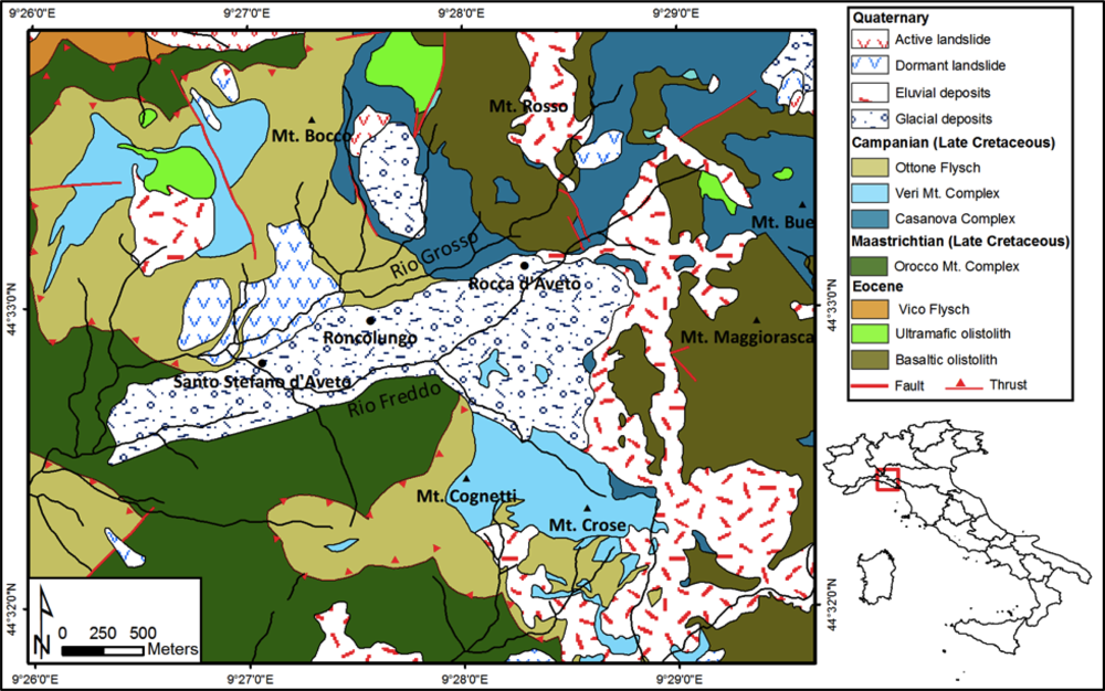
The Santo Stefano d’Aveto village (Figure 1) is located at the boundary between the Emilia-Romagna and Liguria regions in the Po River Basin.
From a geomorphological point of view, the study area is located near the watershed of the Aveto River Basin and the Nure River Basin that sets the limit between the Liguria and the Emilia Romagna regions. The Santo Stefano d’Aveto village is located in an ancient glacial valley, ENE-WSW oriented and bordered on the east by Bue and Maggiorasca mountains, on the north by Bocco and Rosso Mountains and on the south by Crose and Cognetti Mountains. The main reliefs in the area are represented by the Bue and Maggiorasca peaks that reach an altitude of 1,780 m a.s.l. and 1,800 m a.s.l, respectively.
From a geological point of view (Figure 1), the main outcropping lithologies are constituted by sandstones with limestone and marls and ophiolitic rocks, such as basalts and gabbros.
In particular, the main geologic formations that crop out are:
Ottone flysch: calcareous turbidites characterized by intervals of calcareous marls, marly limestone and marls;
Veri complex: shale olistolites in a shale matrix and breccias in sandy matrix;
Casanova complex: ophiolitic sandstones, breccias in clay matrix and breccias in sandy matrix;
Orocco complex: flysch-type formation constituted by calcareous marls, marly limestone and marls.
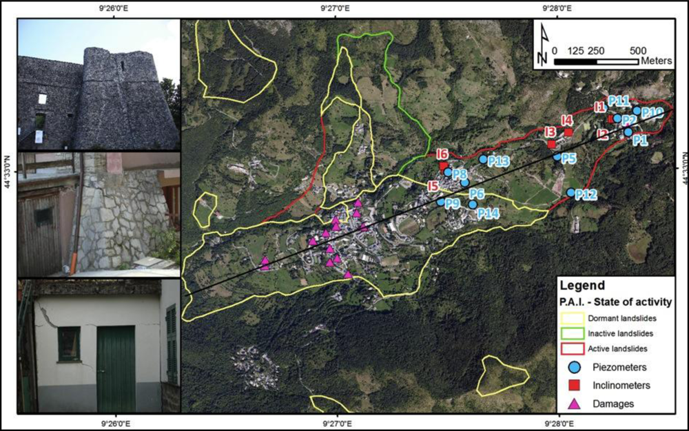
According to the Regional Cartographic map 1:25,000 scale, the Santo Stefano d’Aveto village is located on unsorted glacial deposits constituted of sandstone and ophiolitic clasts in a sandy-silty matrix. Actually, the village is built on an ancient complex landslide that can be defined according to [14] as a complex earth slide-earth flow. The aerial extension of the landslide is 1.3 km2, and the estimated volume is around 10 million cubic meters (Figure 2).
The land cover, which can be easily recognized from the aerial photos, consists in annual and permanent crops, deciduous and mixed forests and a few built-up areas: the main town, Santo Stefano d’Aveto, and two small villages, Roncolungo and Rocca d’Aveto.
The slope angle of the area, derived from a DEM (Digital Elevation Model) with a spatial resolution of 20 m, ranges from 0° to 60°, with an average value of 8°. The maximum values are reached in the upper portion of the landslide, where the main scarp is located.
Two main streams, the Rio Grosso and the Rio Freddo that have set their paths on the right and left side of the landslide, respectively, constitute the local hydrology. The Rio Freddo was subjected to a deviation, which occurred on the left side of the landslide and now crosses the Santo Stefano d’Aveto village and flows within the Rio Grosso.
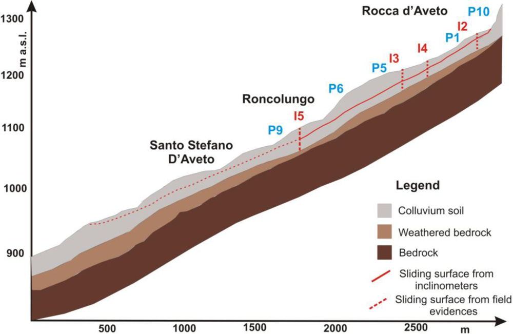
Six boreholes have been drilled to investigate the landslide area and the underground geological setting. The results of the boreholes show that the underground geology is characterized by a three-layer stratigraphy. Starting from the top:
Coarse debris in a sandy-silty matrix with thin layers of clay material and large blocks of ophiolitic rocks. This layer has a thickness ranging from 25 m to 40 m.
Weathered bedrock. This layer has a thickness ranging from 5 m to 20 m.
Bedrock constituted of the sandstones and rubbles of the Complesso di Monte Veri and slates of the Ottone flysch.
A geotechnical characterization has been performed on the first layer of coarse debris showing values of unit weight (γ) ranging from 18 to 22 kN/m3, friction angle (Φ′) ranging from 34° to 37° and effective cohesion (c′) from 0 to 7 kPa.
The investigated area is already included in the Landslide Inventory Map developed within the PAI (Hydrogeomorphological Setting Plan, according to the term suggested by [53]) of the Po River Basin Authority. The landslide has been classified as active in the upslope portion and dormant in the remaining part, where almost all the villages are located.
The velocity of the movement is an extremely slow one (according to the classification given in [14]) and does not represent a high risk to the people, although it poses a major threat to the structural elements at risk. This is also due to the growing economy (mainly based on tourism) of the area that in the last few years has led to an increase in the number of buildings and in infrastructure.
The buildings and the main roads are extensively intersected by cracks and damage and are often subjected to repairing and consolidation works.
2.2. Geotechnical Monitoring
Six inclinometers and eleven piezometers have been installed inside the landslide perimeter (Figure 2) during a geotechnical campaign carried out from 2000 to 2006.
The inclinometric measurements acquired by the instruments are reported in Table 1. The I1, I3 and I5 were installed in 2001, with measurements that span the temporal interval from January 2001 to September 2004. In 2004, three more instruments were added, I2, I4 and I6, which have been measured until September 2006. All the inclinometers reached failure.
The inclinometric measurements have allowed reconstruction of the depth of the sliding surface (Table 1, Figure 3). The landslide affects the first layer of material composed of colluvium soil made of debris in a sandy-silty matrix. Thin layers of clay material are located inside the soil, and they can possibly represent the potentially slip surface. The inclinometric monitoring of the landslide highlights that the slip surface is located at about 10 m of depth in the upslope portion of the landslide and at about 20 m of depth near Santo Stefano d’Aveto village (Table 1). In general, the depth of the slip surface increases from the upper to the lower portion of the landslide.
For each inclinometer, the cumulative displacement in the reference period and the annual mean velocity are reported in Table 1. The highest velocities are measured in the I1 inclinometer located in Rocca d’Aveto.
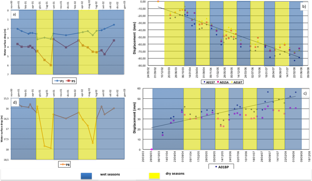
The piezometric monitoring has been carried out from 2000 to 2006 in eleven piezometers with monthly acquisitions. The monitoring has highlighted that there is a free water table in the debris cover and that the average depth of the piezometric surface ranges from a few meters in the upper portion of the landslide to around 20 m at the toe. The measurements present a seasonal variability with a water table lowering during dry seasons and rising in the wet season. The most significant time series of water level depth are reported in Figure 8.
2.3. PSI Data
Characterization and monitoring of the Santo Stefano d’Aveto landslide have been carried out by using long stacks of satellites Synthetic Aperture Radar (SAR) images.
SAR satellite imagery in the C band (5.6 cm wavelength; frequency 5.3 GHz), acquired by the European Space Agency (ESA) satellites ERS1/2 and ENVISAT, were employed for the reconstruction of the history and spatial patterns of the Santo Stefano landslide (Table 2).
These four stacks were processed with the PSInSAR™ approach, the first technique specifically implemented for the processing of multi-temporal radar imagery [19]. The PSInSAR™ analysis provided estimates of yearly deformation velocity, referring to both historical (ERS images) and recent (ENVISAT images) scenarios, allowing the analysis of past and recent ground deformation.
APSA mode processing resulted in four different datasets (i.e., one for each stack), finally leading to the generation of deformation velocity maps and a displacement time series of point-wise targets for which a sixteen-year-long displacement history was reconstructed.
Unlike conventional DInSAR techniques, multi-interferometric analysis generates displacement time-series for individual radar targets (i.e., the Persistent Scatterers, PS®), generally assuming a linear model of deformation [19,24]. Accuracy ranges from 1 to 3 mm on single measurements in correspondence to each SAR acquisition and between 0.1 and 1 mm/yr for the Line of Sight (LOS) deformation rate [20]. Time series of ground deformation are ideally suited to define the landslide behavior, to monitor temporally continuous ground motions and to observe kinematic responses to triggering factors. Output results of a Permanent Scatterers analysis (i.e., deformation field maps and time series of displacement) are relative both in time and space.
The reference points of the four stacks—to which displacement measurements are computed—were selected 1.5 km far away from Santo Stefano, over marl formations devoid of ground deformation. It is clear that proper selection of the reference point is of fundamental importance within the PSI processing chain: besides the phase coherence throughout the dataset, the selected point has to be chosen within areas unaffected by ground motions in order to avoid the retrieval of an unreal pattern of deformation.
PSI techniques use large stacks of SAR images to generate many single-pair interferograms with respect to one master image, to reconstruct, acquisition per acquisition, the displacement history of reflective targets. Hence, each measurement is referred temporally to a unique reference image, chosen to minimize the effects of spatial and temporal baselines and to maximize the total coherence of the interferometric stack and to keep as low as possible the dispersion of the normal baseline values.
As reported in Table 2, for both ERS and ENVISAT datasets in ascending geometry, the number of natural benchmarks detected is smaller than in the descending orbits. Moreover, also the absolute values of registered velocities are lower in the ascending geometry. This is mainly related to the SAR looking geometry with respect to the topographic aspect and to the direction of slope movement.
The target points within the Santo Stefano landslide have a high density, particularly in correspondence of the urban fabric of the village, because the wide availability of bright, stable (i.e., phase coherent) man-made objects.
More than 400 point-wise measurements points have been retrieved for the 1.3 km2 wide landslide area, processing 78 ERS descending images and retrieving phase information from “natural” target already present on the ground. It is clear that ground-based methods for landslide monitoring, despite their robustness and reliability, are not able to provide such a large density of measurement points as the PSI technique does. Conventional techniques (e.g., GPS, optical leveling, inclinometric tubes), relying on materialization of physical benchmarks in representative points of the landslide area and on repeated measurement acquisition campaigns, are designed to cover a limited extension of the affected area and to provide a static picture of deformation history. By increasing density, coverage and frequency of measurements, PSI technique contributes to improving the overall understanding and confidence on landslide behavior and kinematics.
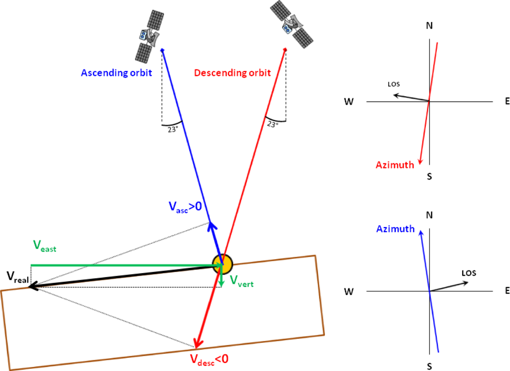
InSAR-based displacements are 1D measurements. SAR sensors are side-looking radar and operate with a LOS direction tilted with respect to the vertical direction. Because of the rather small incidence angle (usually between 23° and 45°), the sensor is much more sensitive to vertical deformation than to horizontal deformation. Hence, the resulting datasets can estimate only a small component of the 3D real motion of the landslide, i.e., the projection along the satellite LOS. Under the assumption of absence of N-S deformation components, combining ascending and descending information permits one to extract the vertical and horizontal (in the east-west direction) components of the movement and, consequently, the real vector of displacement [54–56] (Figure 4).
Generally, to combine ascending and descending datasets and extract the vertical and east-west components of a specific point on the ground, it is necessary to identify a radar target acting as a scatterer in both acquisition geometries. Practically, identification of the same radar target in both the datasets by using medium resolution SAR sensors (i.e., ERS1/2 and ENVISAT with a range and azimuth resolution of 25 m and 5 m, respectively) is often a challenge. Typical values of positioning precision are 7 m and 2 m for the East-West and North-South direction, respectively, for PS® less than 1 km from the reference point and considering a five-year-long dataset of C-band radar images. Precision on elevation values is 1.5 m.
Due to this low spatial resolution and to the poor georeferencing accuracy, it is often difficult not only to identify exactly what object is acting as the “persistent scatterer”, but even if the scattering object is identified, it is then difficult to detect which part of the object is actually scattering.
To overcome this limitation, it was necessary to resample the datasets of PS® points by means of a regular grid with 50 m intervals. For each grid cell and for both the ascending and descending geometries, the mean value of the velocities of the radar targets contained within the cell is calculated. Hence, a synthetic Permanent Scatterrer is generated, with associated ascending (VA) and descending (VD) velocity estimates. Using the synthetic values and taking into account the orientation of the employed LOS, the vertical (VV) and east-west (VE) ground velocity components were estimated, by solving—cell by cell—the following formulas [57]:
LOS of ERS1/2 and ENVISAT satellites have identical acquisition geometries and are characterized by incidence angle (θ), θA = θD ∼ 23°.
3. Results
3.1. PSI Landslide Characterization and Monitoring
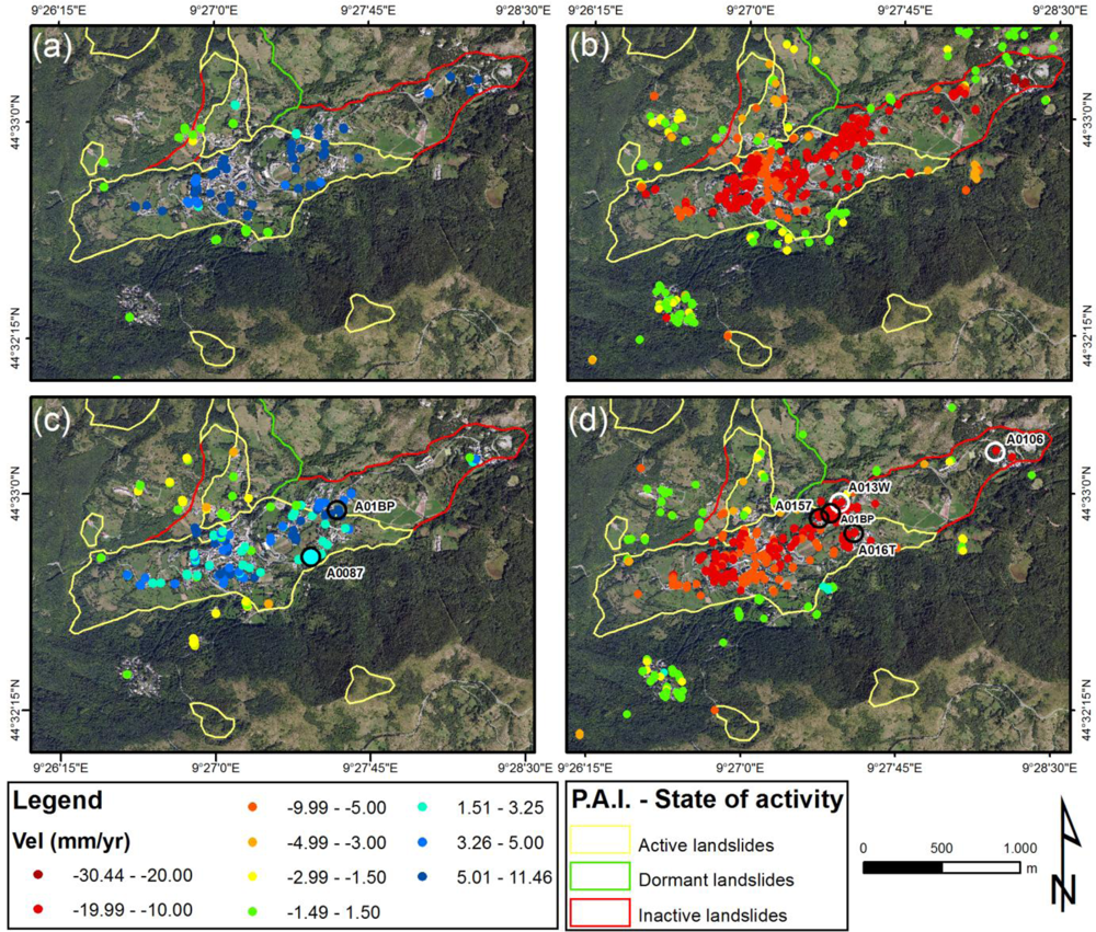
In Figure 5, the distribution of PS® points within the landslide is shown. LOS deformation rates between +1.5 and −1.5 mm/yr (close to the sensitivity of the PSI technique) reflect motionless areas. PS®s with LOS velocities < −1.5 mm/yr indicate surface deformation motion away from the satellite, while LOS deformation rates > +1.5 mm/yr reflect movements towards the satellite. The color scale gradations from yellow to dark red and from light blue to violet represent increasing deformation rates.
The average absolute velocity of the PS®s ERS descending within the landslide is 12.3 mm/yr, while the maximum value is 37.9 mm/yr (Table 2). The highest velocities, up to 35 mm/yr, have been generally measured in the upslope zone of the landslide, where Rocca d’Aveto is located. In the middle part of the slope, where the village of Roncolungo is situated, the velocities vary in the range of 10–20 mm/yr. In correspondence with the Santo Stefano village, slope velocities vary from a minimum of 6 mm/yr to a maximum of 16 mm/yr. The average velocity of the ERS ascending dataset is around 6 mm/yr along the satellite LOS, with peaks, recorded nearby the Rocca d’Aveto, up to 11 mm/yr. As for the ERS descending dataset, the PS®s velocities are decreasing from Rocca d’Aveto to Santo Stefano village.
The PS® ENVISAT descending dataset shows a mean velocity (in absolute value) of 10.2 mm/yr with a peak of 19.8 mm/yr. Velocities of PS®’s in Rocca d’Aveto are up to 15 mm/yr, while in Roncolungo, they range from 10 mm/yr to 15 mm/yr, and in Santo Stefano d’Aveto, they range from 5 mm/yr to15 mm/yr. The ENVISAT ascending dataset has a mean value of velocity of 3.5 mm/yr, while the maximum value is around 7 mm/yr. Also for the ENVISAT dataset, deformation rates decrease moving down-slope.
The measurements recorded during the different time periods (1992–2000 and 2002–2008) and through different acquisition geometries—descending and ascending—are consistent and confirm that the recorded ground movement is related to a slope movement with a NE-SW direction component.
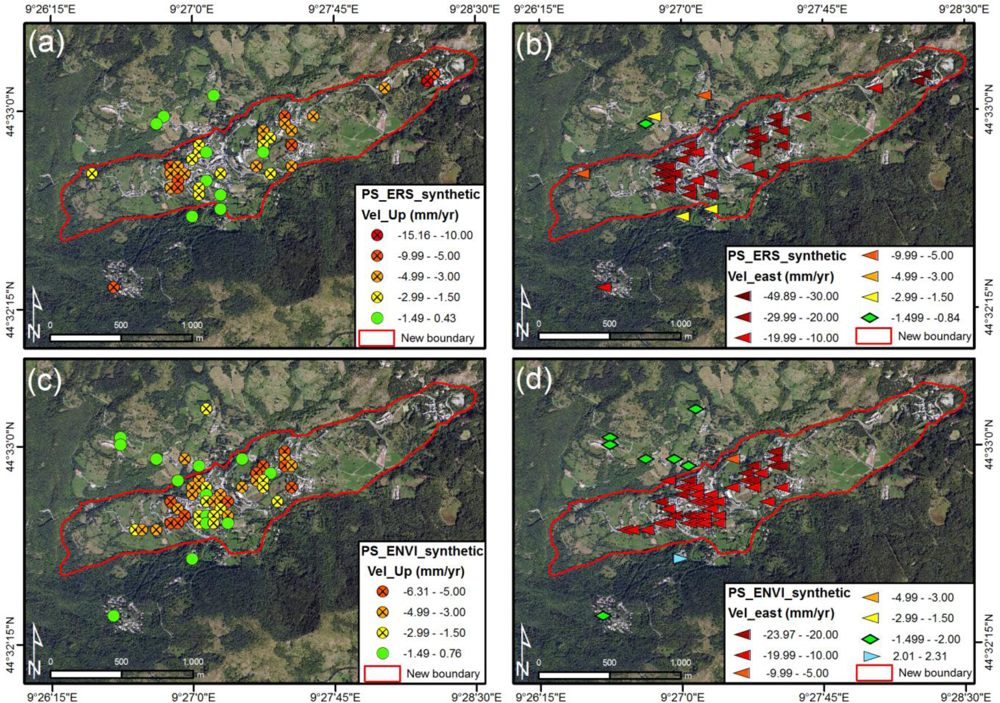
The results of the combination of ascending and descending data both for ERS and ENVISAT datasets is shown in Figure 6, where PS®’s with positive velocities indicate surface deformation motion upward and eastward, while negative deformation rates reflect movements downward and westward.
The re-projection of LOS velocity into its horizontal and vertical components reveals that the Santo Stefano landslide is characterized by predominant horizontal components, consistent with a strong westward movement, just as expected. Hence, land deformation is mainly horizontal, with negative velocity values ranging between 20 mm/yr and 30 mm/yr with peaks up to 49 mm/yr in the ERS dataset and between 10 mm/yr and 20 mm/yr in the ENVISAT dataset. The landslide is characterized by low vertical displacements (on the order of a few mm/yr), both in ERS and ENVISAT dataset. It is worth noting that in the upslope portion of the landslide, in the ERS time period, higher downward velocities were registered, with a peak up to 15 mm/yr.
This pattern of movement is typical of those sliding masses commonly involving two or more of the classes of landslide typologies. In particular, observed displacements in the uppermost part of the landslide body are consistent with a downward movement usually observed in rotational slides: as the mass of material moves down slope along the concave slip surface that is not structurally-controlled, it rotates downward, leaving a large main head scarp. Moving down-slope, the phenomenon evolves into a translational slide, as the landslide mass moves along a roughly planar surface with little or no internal deformation, as testified by negligible vertical deformation rates. In its lowermost part, the slide further transforms into an earth flow, as the material starts to lose coherence.
In sum, the pattern of movement of the Santo Stefano landslide, as observed by InSAR monitoring, supports and constrains the interpretation of the landslide itself and the definition of the style of movement. The landslide is defined as a complex phenomenon, started as a roto-translational slide affecting the source area, which evolves downhill into an earth flow.
3.2. PSI versus Geotechnical Monitoring
The time series of ENVISAT data, spanning the time period from 2002 to 2008, have been compared with the inclinometers, whose measurements cover a period from 2001 to 2006 and with piezometers spanning from 2000 to 2006. Time series are displayed as time-displacement diagrams. On the x-axis, the dates of acquisition are reported, ranging from 06/07/2003 to 29/06/2008, and on the y-axis are the displacement values taken along the line of sight of the satellite.
For the comparison of PSI data with inclinometers, the descending acquisition has been employed, because of the large amount of available images.
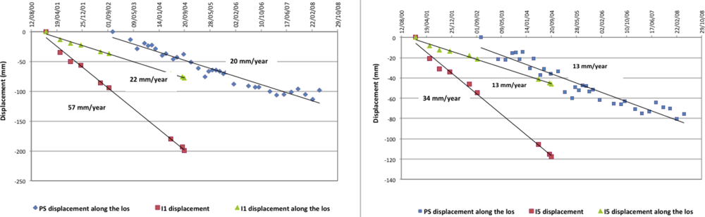
The I1 inclinometer has been compared with the PS® A0106, whereas the I5 has been compared with the PS® A013W (Figure 7). The distance between PS® and inclinometer is 15 m and 40 m, respectively. The actual locations of inclinometers and PS® points are reported in Figures 2 and 5, respectively. In both cases, as expected, it is observed that the average velocities of the inclinometers are consistently higher than the PS® average velocity. This is because the radar benchmark displacement is measured along the LOS of the satellite, so it can measure only a component of the real movement vector, whereas the inclinometer measures the actual displacement along the maximum slope angle direction.
In order to perform a more representative comparison, the displacement vector of the inclinometers has been projected along the LOS using a simple trigonometry equation:
The results confirm that the displacements measured along the LOS underestimate the real movement measured by the inclinometer along the maximum slope angle direction. In particular, for the I1 instrument, the velocity value along the maximum slope angle is 57 mm/yr, while the component along the LOS is 22 mm/yr. The I5 instrument shows a velocity along the maximum slope angle of 34mm/yr, while along the LOS it is 13 mm/yr.
In both cases, the computed velocity values of the inclinometers along the LOS (22 mm/yr for I1 and 13 mm/yr for I5) show values quite similar to PS® mean velocities.
The PSI data have been compared also with the piezometer measurements in order to define the relationship among the landslide displacements and the triggering factors. Both ascending and descending orbits of PSI ENVISAT data have been considered for the comparison. The PS®s and the piezometers selected for the comparison are highlighted in Figures 5 and 2, respectively.
In general, it can be observed that displacements detected by the descending orbit move away from the LOS during the autumn season and move toward the LOS during the summer season (Figure 8(b)). On the contrary, the ascending orbit displacements move towards the LOS in autumn and away from the LOS in summer (Figure 8(c)). Time series of piezometers measurements reported in Figure 8(a–d) shows that water level rises during wet seasons and lowers in dry seasons. Therefore, the comparison between the PSI time series and piezometers time series highlights that:
Wet seasons: rise of the water table level in the piezometers, increase of the displacement rates from PSI technique.
Dry seasons: lowering of the water table level in the piezometers, decreasing of the displacement rates from PSI technique.
4. Discussion
The outcomes of this work suggest that the PSI technique can have a high potential in the field of landslide monitoring, but the use of only this technique for this purpose needs to be carefully evaluated [58]. Even if the use of the PSI technique can overcome some limitations of the conventional monitoring techniques (e.g., large extension of the area to be monitored and high costs, inaccessibility of the area, problems of installation and maintenance) it cannot replace in situ measurements [58].
Considering ERS and ENVISAT LOS orientation, the slope movement with a NE-SW direction (revealed by the combination of ascending and descending geometries) and the orientation of the slope, LOS mean displacement rates measured with the interferometric analysis represent only a small percentage of the real occurred displacements. Hence, as expected and demonstrated by [59] for a subsiding mining area and by [60] for tectonic movements, the real deformation rates occurring between 1992 and 2008 were much higher than those observed by interferometric technique.
Besides the intrinsic 1D measurement capacity of InSAR approaches, the underestimation of occurred displacements is also due to the range of velocity actually detectable, to the kinematic behavior of the investigated phenomenon and to the linear model used during the PSI processing. It is worth recalling that in most PSI applications, without any a priori knowledge about deformation, a simplified model (which assumes a linear, constant-rate phase variation with time) is usually assumed to retrieve ground motion. The assumption of the linear model of displacement for SAR interferometry processing is adequate for steady state displacement with respect to image sampling. In most of the cases, geological processes, such as landslides, cannot be described with a linear trend. By using a predefined linear displacement model, the extraction of phase variations related to displacement for each scatterer can be inaccurate: during phase unwrapping the non-linear component of deformation becomes indistinguishable and is included into other phase terms, leading to the underestimation of the actual deformation patterns. This limitation, known as aliasing, is particularly relevant for low PS® density and/or low temporal sampling with respect to deformation and/or geological processes with strong deformation magnitudes. Moreover, during phase unwrapping, ambiguity related to the discrete interval sampling (2π) of the wrapped phase can remain unsolved: indeed, without any further information on the behavior of ground deformation, the maximum displacement between two successive acquisitions (the temporal sampling of ERS1/2 and ENVISAT scenes is 35 days) and two close PS®’s of the same dataset is limited to a quarter of the wavelength (λ/4, i.e., 1.4 cm for C-band sensors).
Considering the aforementioned limitations of the techniques (phase ambiguity, long revisiting time of employed satellites and measuring capacity limited to smooth deformation fields) and the intermittent behavior of the landslide, it is possible that seasonal pulse produced phase ambiguity, imperfect linearity of the deformation and, finally, displacements exceeding the λ/4 threshold. It is therefore reasonable to expect a general underestimation of the deformation actually occurred in 1992–2008.
For all the above reasons, the qualitative and quantitative integration of ground-based monitoring data and PSI data can provide sound results for landslide characterization. It is worth underlying that punctual information deriving from inclinometers can help in defining the actual location of the sliding surface and the involved volumes. On the other hand, the measuring of pore water pressure conditions or water table level can suggest correlation between the deformation patterns and the triggering factors.
In summary, in landslide monitoring, the joint use of remote sensing monitoring techniques and ground-based ones are recommended.
5. Conclusion
In this work, the characterization and monitoring of the Santo Stefano d’Aveto landslide has been carried out integrating PSI data and conventional monitoring techniques. The PSI analysis has been performed using ascending and descending SAR scenes from ERS-1/-2 (1992–2001) and ENVISAT (2002–2008) satellites. All the datasets have been processed in the advanced mode APSA. Conventional geotechnical monitoring has been carried out from 2000 to 2006 by means of inclinometers and piezometers.
The analysis of PSI datasets highlights that the velocity within the landslide shows a general decrease from the upper to the lower part of the landslide. In particular, for ERS data, the maximum-recorded value was about 38 mm/yr in the Rocca d’Aveto area, while in the Santo Stefano village, the velocity reached the value of 12 mm/yr. Even for ENVISAT data, the maximum value was recorded in Rocca d’Aveto, with rates up to 20 mm/yr. On the other side, the deformation recorded within the Santo Stefano d’Aveto village ranged from 5 mm/yr to 15 mm/yr.
PSInSAR™ analysis for the temporal interval from 1992 to 2008 allowed the changing of the state of activity of the landslide and the defining of the landslide intensity in terms of velocity. According to the methodology proposed in [61], the SW portion of the landslide, in correspondence to Santo Stefano d’Aveto village, previously classified as dormant, can be now classified as active, since both ERS and ENVISAT datasets show velocities higher than 1.5 mm/yr, which is the PSI technique sensitivity. Concerning the upper part of the landslide, near Rocca d’Aveto, the state of activity has been confirmed as active. According to [14] and on the basis of the PSI data, landslide velocity can be defined as very slow. Moreover, it has been possible to confirm almost all the boundaries, except for a small change located in the northern side of Santo Stefano d’Aveto village. The new landslide map is shown in Figure 6.
By combining information on landslide displacements, acquired by ascending and descending geometries, it has been possible to highlight a predominant horizontal component, consistent with a strong westward direction of the movement. Moreover, vertical deformation in the upper part of the landslide body is thought to reflect a rotational movement, evolving downhill into an earth flow.
The APSA analysis has provided information about the temporal evolution of specific target points. The majority of both the ERS and ENVISAT time series have shown a seasonal trend.
The results of the geotechnical monitoring have been compared to PSI data. A comparison between the deformation measured by the PSI techniques and the inclinometric acquisitions has been performed examining the velocity measurements along the same line of sight. In particular, in order to perform the comparison, the displacements of the inclinometers, taken along the maximum slope angle direction, have been plotted along the line of sight of the satellite. The results show that the displacements measured by the two different types of techniques are consistent.
The comparison of the PS® results and the in situ monitoring by inclinometers shows that the PS® analysis is a valuable technique to monitor landslide deformations, since for landslide affecting urban areas, it can provide plenty of ground measuring points with time-series deformations. On the other hand, it is important to note that for non-urban landslides, the number of radar benchmarks can be very low.
The comparison of PSI data with piezometers measurements has allowed the relating of the seasonal trend of the time series deformations with water table level fluctuations. In particular, it has been observed that in wet seasons, the rise of the water table level in the piezometers led to an increase in the displacement rates observed by the PSI technique, while in dry seasons, the lowering of the water table level in the piezometers resulted in a decrease of the displacement rates detected by the PSI technique. These observations allow for some preliminary considerations on landslide triggering conditions; therefore, an increase in the deformation rates can be related to seasonal variations in the water table level, i.e., the water pressure conditions.
Based on the above-mentioned results, some general guidelines on the applications of PSI to monitor landslides can be derived. Even though PSI analysis is a valuable technique to monitor landslides, some expedients have to take into account to obtain sound results: (i) correct reconstruction of the actual displacement vector, i.e., the vertical component (VV) and the horizontal E-W component (VE) trough—the combined use of ascending and descending geometry—and (ii) reconstruction of the link between surface and subsurface displacements combing the PSI results with local underground displacements measures (such as inclinometer reading) in order to compare the PSI-based surface velocities with the actual 3D vector at different depths in the landslide body.
Acknowledgments
The Terrafirma project has funded the SAR imagery processing, as well as the geological interpretation presented in this paper. The project is one of many services being supported by the Global Monitoring for Environment and Security (GMES) Service Element Program, promoted and financed by the European Space Agency (ESA). The authors gratefully acknowledge TeleRilevamento Europa (TRE) for having processed SAR data. The authors also acknowledge the Regione Liguria for providing the geotechnical monitoring data and six anonymous referees for their helpful and valuable revisions.
References
- Mantovani, F.; Soeters, R.; van Westen, C. Remote sensing techniques for landslide studies and hazard zonation in Europe. Geomorphology 1996, 15, 213–225. [Google Scholar]
- Farina, P.; Colombo, D.; Fumagalli, A.; Marks, F.; Moretti, S. Permanent Scatterers for landslide investigations: outcomes from the ESA-SLAM project. Eng. Geol 2006, 88, 200–217. [Google Scholar]
- Corominas, J.; Moya, J.; Lloret, A.; Gili, J.A.; Angeli, M.G.; Pasuto, A.; Silavno, S. Measurement of landslide displacements using a wire extensometer. Eng. Geol 2000, 55, 149–166. [Google Scholar]
- Angeli, M.; Pasuto, A.; Silvano, S. A critical review of landslide monitoring experiences. Eng. Geol 2000, 55, 133–147. [Google Scholar]
- Gili, J.A.; Corominas, J.; Rius, J. Using Global Positioning System techniques in landslide monitoring. Eng. Geol 2000, 55, 167–192. [Google Scholar]
- Cotecchia, V.; Grassi, D.; Merenda, L. Fragilità dell’area urbana occidentale di Ancona dovuta a movimenti di massa profondi e superficiali ripetutisi nel 1982. Geologia Applicata e Idrogeologia 1995, 30, 633–657. [Google Scholar]
- Cotecchia, V. La Grande Frana di Ancona: La Stabilità del Suolo in Italia: Zonazione Sismica-Frane. Proceedings of Atti dei Convegni Lincei, 1997, Roma, Italy, 30–31 May 1996; pp. 187–259.
- Kaab, A. Photogrammetry for early recognition of high mountain hazards: New techniques and applications. Phys. Chem. Earth 2000, 25, 765–770. [Google Scholar]
- Bitelli, G.; Dubbini, M.; Zanutta, A. Terrestrial laser scanning and digital photogrammetry techniques to monitor landslide bodies. Int. Arch. Photogram. Remote Sens. Spat. Inform. Sci 2004, 35, 246–251. [Google Scholar]
- Fanti, R.; Gigli, G.; Lombardi, L.; Tapete, D.; Canuti, P. Terrestrial laser scanning for rockfall stability analysis in the cultural heritage site of Pitigliano (Italy). Landslides 2012, 5, 1–12. [Google Scholar]
- Gabriel, A.K.; Goldstein, R.M.; Zebker, H.A. Mapping small elevation changes over large areas: Differential radar interferometry. J. Geophys. Res 1989, 94, 9183–9191. [Google Scholar]
- Massonnet, D.; Feigl, K.L. Radar interferometry and its application to changes in the Earth’s surface. Rev. Geophys 1998, 36, 441–500. [Google Scholar]
- Zebker, H.A.; Goldstein, R.M. Mapping from interferometric synthetic aperture radar observations. J. Geophys. Res 1986, 91, 4993–4999. [Google Scholar]
- Cruden, D.M.; Varnes, D.J. Landslide Types and Processes. In Landslides: Investigation and Mitigation, Special Report 247-Transportation Research Board, National Research Council; Turner, A.K., Schuster, R.L., Eds.; National Academy Press: Washington, DC, USA, 1996; pp. 36–75. [Google Scholar]
- Lu, P.; Casagli, N.; Catani, F.; Tofani, V. Persistent Scatterers Interferometry Hotspot and Cluster Analysis (PSI-HCA) for detection of extremely slow-moving landslides. Int. J. Remote Sens 2012, 33, 466–489. [Google Scholar]
- Righini, G.; Pancioli, V.; Casagli, N. Updating landslide inventory maps using Persistent Scatterer Interferometry (PSI). Int. J. Remote Sens 2012, 33, 2068–2096. [Google Scholar]
- Tofani, V.; Segoni, S.; Agostini, A.; Catani, F.; Casagli, N. Technical note: Use of remote sensing for landslide studies in Europe. Nat. Hazards Earth Syst. Sci 2013, 13, 1–12. [Google Scholar]
- Ferretti, A.; Prati, C.; Rocca, F. Nonlinear subsidence rate estimation using Permanent Scatterers in differential SAR interferometry. IEEE Trans. Geosci. Remote Sens 2000, 38, 2202–2212. [Google Scholar]
- Ferretti, A.; Prati, C.; Rocca, F. Permanent Scatterers in SAR interferometry. IEEE Trans. Geosci. Remote Sens 2001, 39, 8–20. [Google Scholar]
- Colesanti, C.; Ferretti, A.; Prati, C.; Rocca, F. Monitoring landslides and tectonic motions with the Permanent Scatterers Technique. Eng. Geol 2003, 68, 3–14. [Google Scholar]
- Ferretti, A.; Fumagalli, A.; Novali, F.; Prati, C.; Rocca, F.; Rucci, A. A new algorithm for processing interferometric data-stacks: SqueeSAR™. IEEE Trans. Geosci. Remote Sens 2011, 99, 1–1. [Google Scholar]
- Hooper, A.; Zebker, H.; Segall, P.; Kampes, B. A new method for measuring deformation on volcanoes and other natural terrains using InSAR persistent scatterers. Geophys. Res. Lett 2004, 31, L23611. [Google Scholar]
- Hooper, A.; Segall, P.; Zebker, H. Persistent scatterer interferometric synthetic aperture radar for crustal deformation analysis, with application to Volcan Alcedo, Galapagos. J. Geophys. Res 2007, 112, B07407. [Google Scholar]
- Werner, C.; Wegmuller, U.; Strozzi, T.; Wiesmann, A. Interferometric Point Target Analysis for Deformation Mapping. Proceedings of IEEE International Geoscience and Remote Sensing Symposium (IGARSS’03), Toulouse, Francia, 21–25 July 2003; pp. 4362–4364.
- Strozzi, T.; Wegmuller, U.; Keusen, H.R.; Graf, K.; Wiesmann, A. Analysis of the terrain displacement along a funicular by SAR interferometry. IEEE Trans. Geosci. Remote Sens 2006, 3, 15–18. [Google Scholar]
- Mora, O.; Mallorqui, J.J.; Broquetas, A. Linear and nonlinear terrain deformation maps from a reduced set of interferometric SAR images. IEEE Trans. Geosci. Remote Sens 2006, 41, 2243–2253. [Google Scholar]
- Lanari, R.; Mora, O.; Manunta, M.; Mallorqui, J.J.; Berardino, P.; Sansosti, E. A small baseline approach for investigating deformation on full resolution differential SAR interferograms. IEEE Trans. Geosci. Remote Sens 2004, 42, 1377–1386. [Google Scholar]
- Berardino, P.; Fornaro, G.; Lanari, R.; Sansosti, E. A new algorithm for surface deformation monitoring based on small baseline differential SAR interferograms. IEEE Trans. Geosci. Remote Sens 2003, 40, 2375–2383. [Google Scholar]
- Casu, F.; Manzo, M.; Lanari, R. A quantitative assessment of the SBAS algorithm performance for surface deformation retrieval. Remote Sens. Environ 2006, 102, 195–210. [Google Scholar]
- Crosetto, M.; Biescas, E.; Duro, J.; Closa, J.; Arnaud, A. Generation of advanced ERS and Envisat interferometric SAR products using the Stable Point Network technique. Photogramm. Eng. Remote Sensing 2008, 74, 443–451. [Google Scholar]
- Herrera, G.; Notti, D.; Garcia-Davalillo, J.C.; Mora, O.; Cooksley, G.; Sanchez, M.; Arnaud, A.; Crosetto, M. Analysis with C- and X-band satellite SAR data of the Portalet landslide area. Landslides 2011, 8, 195–206. [Google Scholar]
- Costantini, M.; Falco, S.; Malvarosa, F.; Minati, F. A New Method for Identification and Analysis of Persistent Scatterers in Series of SAR Images. Proceedings of IEEE International Geoscience & Remote Sensing Symposium (IGARSS’08), Boston, MA, USA, 6–11 July 2008; pp. 449–452.
- Perissin, D.; Wang, T. Repeat-pass SAR interferometry with partially coherent targets. IEEE Trans. Geosci. Remote Sens 2012, 50, 271–280. [Google Scholar]
- Colesanti, C.; Wasowski, J. Investigating landslides with space-borne Synthetic Aperture Radar (SAR) interferometry. Eng. Geol 2006, 88, 173–199. [Google Scholar]
- Canuti, P.; Casagli, N.; Ermini, L.; Fanti, R.; Farina, P. Landslide activity as a geoindicator in Italy: Signifcance and new perspectives from remote sensing. Environ. Geol 2004, 45, 907–919. [Google Scholar]
- Crosetto, M.; Monserrat, O.; Cuevas, M.; Crippa, B. Spaceborne differential SAR interferometry: data analysis tools for deformation measurement. Remote Sens 2011, 3, 305–318. [Google Scholar]
- Rott, H. Requirements and Applications of Satellite Techniques for Monitoring Slope Instability in Alpine Areas. Proceedings of Workshop on Risk Mitigation of Slope Instability, Ispra, Italy, 30 September–1 October 2004.
- Paganini, M. The Use of Space-Borne Sensors for the Monitoring of Slope Instability: Present Potentialities and Future Opportunities. Proceedings of Workshop on Risk Mitigation of Slope Instability, Ispra, Italy, 30 September–1 October 2004.
- Rott, H.; Mayer, C.; Siegel, A. On the Operational Potential of SAR Interferometry for Monitoring Mass Movements in Alpine Areas. Proceedings of the 3rd European Conference on Synthetic Aperture Radar (EUSAR 2000), Munich, Germany, 23–25 May 2000; pp. 43–46.
- Refice, A.; Guerriero, L.; Bovenga, F.; Wasowski, J.; Atzori, S.; Ferrari, R.; Marsella, M. Detecting landslide activity by SAR interferometry. Proceeding of ERS-Envisat Symposium, Goteborg, Sweden, 16–20 October 2000.
- Berardino, P.; Costantini, M.; Franceschetti, G.; Iodice, A.; Pietranera, L.; Rizzo, V. Use of differential SAR interferometry in monitoring and modelling large slope instability at Maratea (Basilicata, Italy). Eng. Geol 2003, 68, 31–51. [Google Scholar]
- Singhroy, V.; Molch, K. Characterizing and monitoring rockslides from SAR techniques. Adv. Space Res 2004, 33, 290–295. [Google Scholar]
- Strozzi, T.; Farina, P.; Corsini, A.; Ambrosi, C.; Thüring, M.; Zilger, J.; Wiesmann, A.; Wegmüller, U.; Werner, C. Survey and monitoring of landslide displacements by means of L-band satellite SAR interferometry. Landslides 2005, 2, 193–201. [Google Scholar]
- Meisina, C.; Zucca, F.; Conconi, F.; Verri, F.; Fossati, D.; Ceriani, M.; Allievi, J. Use of permanent scatterers technique for large-scale mass movement investigation. Quatern. Int 2007, 171–172, 90–107. [Google Scholar]
- Fornaro, G.; Pauciullo, A.; Serafino, F. Deformation Monitoring over large areas with Multipass Differential SAR Interferometry: A new approach based on the use of Spatial Differences. Int. J. Remote Sens 2009, 30, 1455–1478. [Google Scholar]
- Prati, C.; Ferretti, A.; Perissin, D. Recent advances on surface ground deformation measurement by means of repeated space-borne SAR observations. J. Geodyn 2010, 49, 161–170. [Google Scholar]
- Peyret, M.; Djamour, Y.; Rizza, M.; Ritz, J.F.; Hurtrez, J.E.; Goudarzi, M.A.; Nankali, H.; Chèry, J.; Le Dortz, K.; Uri, F. Monitoring of a large slow Kahrod landslide in Alborz mounatin range (Iran) by GPS and SAR interferometry. Eng. Geol 2008, 100, 131–14. [Google Scholar]
- Pancioli, V.; Raetzo, H.; Campolmi, T.; Casagli, N. Terrafirma Landslide Services for Europe based on Space-borne InSAR Data. Proceedings of the First World Landslide Forum, Tokyo, Japan, 18–21 November 2008; pp. 81–84.
- Tofani, V.; Catani, F.; Pancioli, V.; Moretti, S.; Casagli, N. Integration of PSI Technique and Conventional Ground-Based Methods for Characterization and Monitoring of Santo Stefano d’Aveto Landslide (Central Italy). Proceedings of the Mountain Risks: bringing Science to Society, Florence, Italy, 24–26 November 2012; pp. 301–330.
- Strozzi, T.; Delaloye, R.; Kääb, A.; Ambrosi, C.; Perruchoud, E.; Wegmüller, U. Combined observations of rock mass movements using satellite SAR interferometry, differential GPS, airborne digital photogrammetry, and airborne photography interpretation. J. Geophys. Res 2010, 115, F1. [Google Scholar]
- Liao, M.S.; Tang, J.; Wang, T.; Balz, T.; Zhang, L. Landslide monitoring with high-resolution SAR data in the Three Gorges region. Sci. China Earth Sci 2012, 55, 590–601. [Google Scholar]
- Regione Liguria-Carta Geologica Regionale (CARG) sc. 1:25000-tav. 215.4-S. Stefano D’Aveto (2006). Availableonline: http://www.cartografia.regione.liguria.it/templateFogliaRC.asp?itemID=30208&level=3&label=INFORMAZIONI%20GEOSCIENTIFICHE (accessed on 30 November 2012).
- Sorriso Valvo, M. Landslide Risk Assessment in Italy. Landslide Hazard and Risk; Glade, T., Anderson, M., Crozier, M.J., Eds.; John Wiley & Sons: Chichester, UK, 2005; pp. 699–732. [Google Scholar]
- Raspini, F.; Cigna, F.; Moretti, S. Multi-temporal mapping of land subsidence at basin scale exploiting Persistent Scatterer Interferometry: Case study of Gioia Tauro plain (Italy). J. Maps 2012, 8, 514–524. [Google Scholar]
- Ferretti, A.; Savio, G.; Barzaghi, R.; Borghi, A.; Musazzi, S.; Novali, F.; Prati, C.; Rocca, F. Submillimeter accuracy of InSAR time series: Experimental validation. IEEE Trans. Geosci. Remote Sens 2007, 45, 1142–1153. [Google Scholar]
- Ng, A.H.-M.; Ge, L.; Zhang, K.; Li, X. Monitoring ground deformation in Beijing, China with Persistent Scatterer SAR Interferometry. J. Geodesy 2012, 86, 375–392. [Google Scholar]
- Fialko, Y.; Simons, M.; Agnew, D. The complete (3-D) surface displacement field in the epicentral area of the 1999 Mw 7.1 Hector Mine Earthquake, California, from space geodetic observations. Geophys. Res. Lett 2001, 28, 3063–3066. [Google Scholar]
- Calò, F.; Calcaterra, D.; Iodice, A.; Parise, M.; Ramondini, M. Assessing the activity of a large landslide in southern Italy by ground-monitoring and SAR interferometric techniques. Int. J. Remote Sens 2012, 33, 3512–3530. [Google Scholar]
- Raucoules, D.; Bourgine, B.; Michele, M.; Le Gozannet, G.; Closset, L.; Bremmer, C.; Veldkamp, H.; Tragheim, D.; Bateson, L.; Crosetto, M.; et al. Validation and intercomparison of persistent scatterers interferometry: PSIC4 project results. J. Appl. Geophys 2009, 68, 335–347. [Google Scholar]
- Cigna, F.; Del Ventisette, C.; Liguori, V.; Casagli, N. Advanced radar-interpretation of InSAR time series for mapping and characterization of geological processes. Nat. Hazard. Earth Sys. Sci 2011, 11, 865–881. [Google Scholar]
- Cigna, F.; Bianchini, S.; Casagli, N. How to assess landslide activity and intensity with Persistent Scatterer Interferometry (PSI): the PSI-based matrix approach. Landslides 2012, 5, 1–17. [Google Scholar]


| Inclinometers | Mean Velocity (mm/yr) | Cumulative Displacement (mm) | Depth of the Sliding Surface (m) |
|---|---|---|---|
| I1 | 57.8 | 200 | 8.5 |
| I2 | 33.8 | 35 | 9 |
| I3 | 31.2 | 100 | 18.5 |
| I4 | 14.7 | 30 | 17 |
| I5 | 34.1 | 120 | 22.5 |
| I6 | 31.6 | 30 | 12.5 |
| Satellite | Orbit | Time Period | Nr PS | Nr Scenes | Mean (mm/yr) | Min (mm/yr) | Max (mm/yr) |
|---|---|---|---|---|---|---|---|
| ERS1/2 | Ascending | 09/07/1992–20/08/2000 | 85 | 27 | 6.1 | 1.3 | 11.5 |
| Descending | 16/05/1992–19/12/2000 | 403 | 78 | 12.3 | 0.42 | 37.9 | |
| ENVISAT | Ascending | 06/07/2003–29/06/2008 | 118 | 30 | 3.5 | 0.69 | 6.95 |
| Descending | 15/10/2002–06/05/2008 | 274 | 33 | 10.2 | 1.0 | 19.8 |
Share and Cite
Tofani, V.; Raspini, F.; Catani, F.; Casagli, N. Persistent Scatterer Interferometry (PSI) Technique for Landslide Characterization and Monitoring. Remote Sens. 2013, 5, 1045-1065. https://doi.org/10.3390/rs5031045
Tofani V, Raspini F, Catani F, Casagli N. Persistent Scatterer Interferometry (PSI) Technique for Landslide Characterization and Monitoring. Remote Sensing. 2013; 5(3):1045-1065. https://doi.org/10.3390/rs5031045
Chicago/Turabian StyleTofani, Veronica, Federico Raspini, Filippo Catani, and Nicola Casagli. 2013. "Persistent Scatterer Interferometry (PSI) Technique for Landslide Characterization and Monitoring" Remote Sensing 5, no. 3: 1045-1065. https://doi.org/10.3390/rs5031045