Enhanced Processing of 1-km Spatial Resolution fAPAR Time Series for Sugarcane Yield Forecasting and Monitoring


Abstract
: A processing of remotely-sensed Fraction of Absorbed Photosynthetically Active Radiation (fAPAR) time series at 1-km spatial resolution is established to estimate sugarcane yield over the state of São Paulo, Brazil. It includes selecting adequate time series according to the signal spatial purity, using thermal time instead of calendar time and smoothing temporally the irregularly sampled observations. A systematic construction of various metrics and their capacity to predict yield is explored to identify the best performance, and see how timely the yield forecast can be made. The resulting dataset not only reveals a strong spatio-temporal structure, but is also capable of detecting both absolute changes in biomass accumulation and changes in its inter-annual variability. Sugarcane yield can thus be estimated with a RMSE of 1.5 t/ha (or 2%) without taking into account the strong linear trend in yield increase witnessed in the past decade. Including the trend reduces the error to 0.6 t/ha, correctly predicting whether the yield in a given year is above or below the trend in 90% of cases. The methodological framework presented here could be applied beyond the specific case of sugarcane in São Paulo, namely to other crops in other agro-ecological landscapes, to enhance current systems for monitoring agriculture or forecasting yield using remote sensing.1. Introduction
Sugarcane (Saccharum spp. L.) is a crop that plays a major role in global agricultural product trades. The increasing importance of this crop is a consequence of its use, not only as food or feed, but also as the basis for biofuel (ethanol) production. Brazil is the main producer worldwide. According to the IGBE (Instituto Brasileiro de Geografia e Estatística), Brazil’s yearly production is 672 million tons, which accounts for almost one third of the total world production. In such a context, there is a clear interest for managers and decision-makers to have tools capable of monitoring continuously the vegetative vigour of the Brazilian sugarcane and providing timely information regarding potential short-term impacts of weather conditions on yield expectations.
Spatial information technologies, and particularly satellite remote sensing methods, constitute valuable means for assessing vegetation status and green biomass accumulation. Regional scale crop monitoring and yield estimation and forecasting have often been done using satellite Earth observation instruments providing frequent (daily or near-daily) information at a coarse spatial resolution (circa 1 km) [1,2]. For sugarcane, satellite observation has more traditionally been used for applications such as classifying different sugarcane varieties using spectral indices [3,4]. The analysis of temporal series has also been used to classify and separate sugarcane clusters from the rest of land use/land cover classes, aiding the assessment of sugarcane expansion in the São Paulo region [5–7]. Within this framework, the Canasat Project [5], developed by INPE (Instituto Nacional de Pesquisas Espaciais, Brazil), is producing sugarcane distribution maps. Recent studies applied remote sensing techniques to monitor sugarcane phenology as well. The contribution of high resolution imagery in the monitoring of the harvest has been investigated [8] and the potential use of spectral vegetation indices to estimate the phenological development has been explored [9]. More recently, the application of time series analysis of Normalized Difference Vegetation Index (NDVI) and climatic indices with the purpose of predicting sugarcane development has also been studied [10].
Valuable information provided by vegetation indices derived from remote sensing imagery has been used as proxies for estimating the presence of green biomass, the vegetative vigor of sugarcane and yield at harvest. Synthetic images constructed from different vegetation indices have been used by [11] to estimate yield on different study plots through a process of normalization against measured values of crop productivity. A slightly different approach was followed by [12], using a method based in the relationship between observed yield and an estimation based on a simple agronomical model incorporating Leaf Area Index (LAI) calculated from remote sensing. Studies based on in situ measurements, e.g., [13], highlight the relationship between sugarcane yield and vegetation indices adjusted by the thermal time. In a context of precision agriculture, information about the NDVI can be used to delineate areas within a field where unequal yields can be expected [14]. More recently, some work [15] based on relationships between NDVI, meteorological indicators and sugarcane yield in the São Paulo region, underlined the reliability of indicators based on spectral indices to access yield at municipality scale.
2. Goal and Objectives
The present work aims to further contribute to the understanding of how remote sensing indicators can predict within-season sugarcane yields at the state level in São Paulo. The relationship between low resolution SPOT-VEGETATION biophysical products, weather data and official state-level yield statistics for São Paulo are studied through different metrics extracted from seasonal time series of fAPAR (fraction of Absorbed Photosynthetically Active Radiation) and weather data over the period 1999–2010. Special attention is paid to the spatial purity of the time series and its influence in the reliability of yield estimations. The possibility of taking into account seasonal changes in phenology associated with differences in the temperature regime is also explored by using thermal time instead of calendar time when computing the fAPAR metrics. Finally, an analysis on the predictive capacity of remote sensing indicators at the different moments of the season is presented.
3. Material and Methods
3.1. Study Site
The study site is the state of São Paulo, which in itself is responsible for 60% of the Brazilian sugarcane production. The last decade has witnessed a rise of 76% in the surface of São Paulo dedicated to this crop, resulting in a total extension of 4.8 million ha of sugarcane. Sugarcane is a semi-perennial crop with two basic types of production cycles. The plant-cane cycle starts when a stalk cutting is planted and finishes with the first harvest, which typically takes place either after 12 months, or after 18 months. The ratoon, or stubble cane, is the cane that re-sprouts from the piece of cane left over after plant-cane harvest. The ratoon cycle continues for 1 year until the next harvest, and the cycle repeats yearly with each successive ratoon crop. However, the ratoon cane of the currently used cultivars results in increasingly lower yields from year to year, and after around 5 years they become economically unfeasible to maintain [16]. At that point, the crop undergoes renewal, or renovation, by which it is ploughed out and then re-planted with new stalk cuttings.
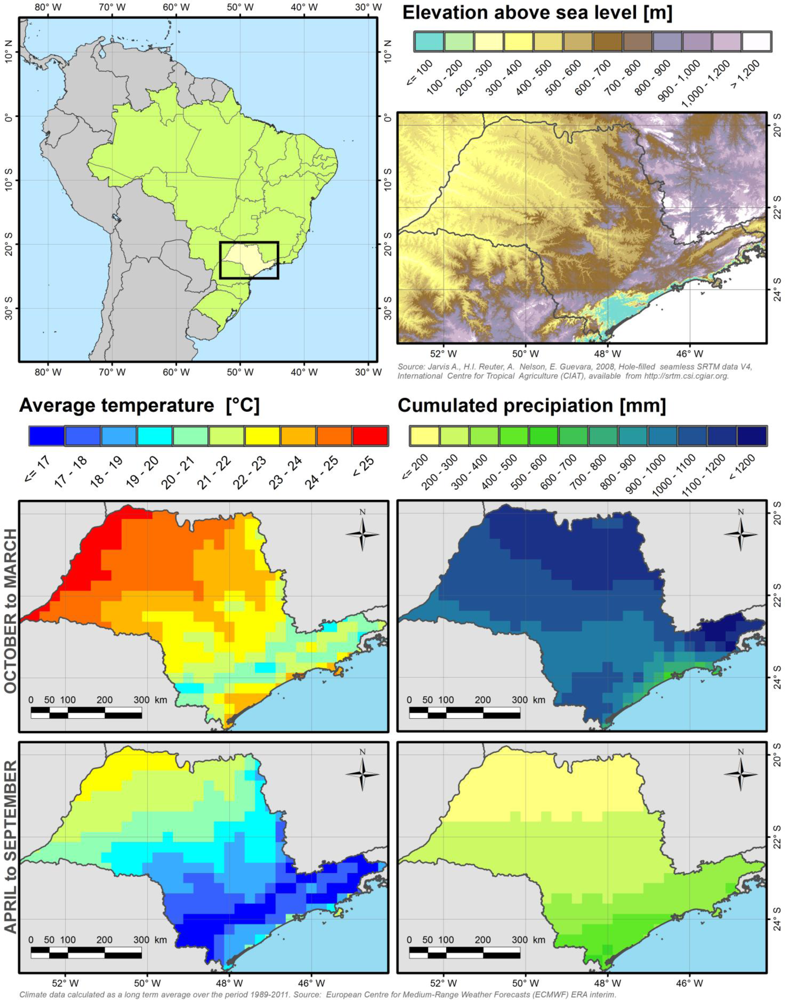
The climate of São Paulo state is tropical to subtropical, which is optimal for sugarcane growth. Total rainfall is about 1,300 mm per year concentrated in a humid season which extends from October to March, when average temperatures oscillate around 23 °C with a strong SE-NW gradient (see Figure 1). During the dry period between July and September, temperatures drop to approximately 19 °C. According to the Köppen climate classification system, the state can be divided approximately in two along an E-W division between the two main climates: tropical savannah (Af) in the North and humid subtropical climate (Cfa) in the South.
3.2. Sugarcane Spatial Distribution
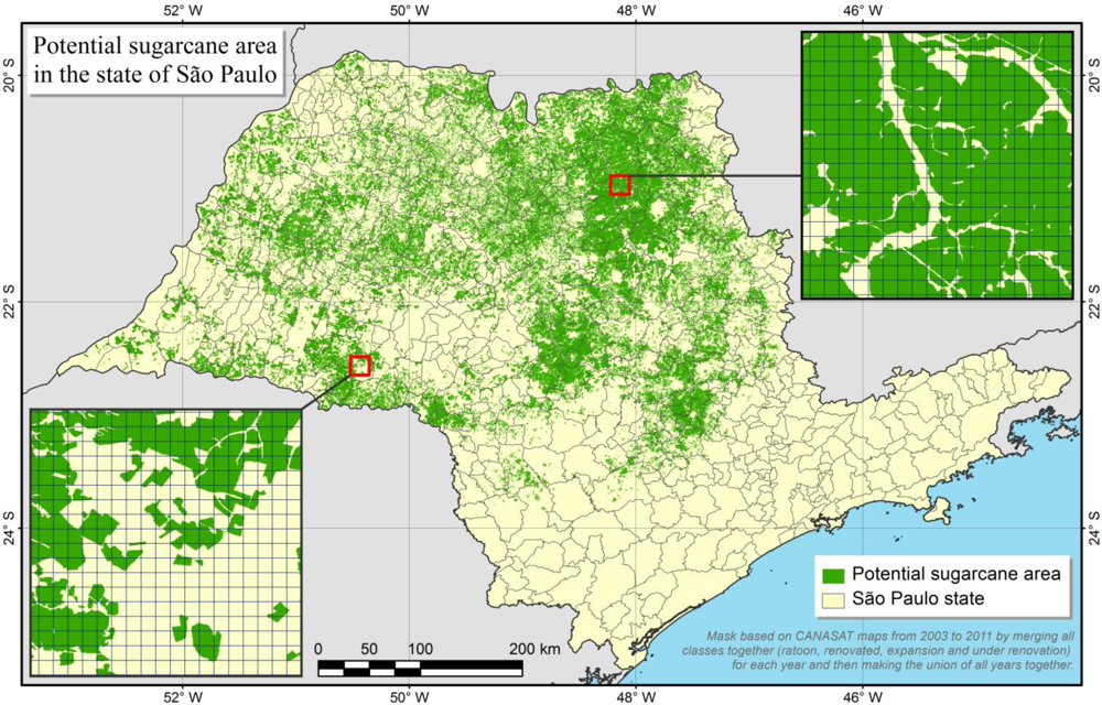
The distribution of sugarcane is not uniform in the territory. It is concentrated in the Central and North-eastern parts of the state (see Figure 2). In this study, the spatial location of sugarcane is obtained based on maps produced in the framework of the Canasat Project [5,8]. These maps are created on a yearly basis using freely available remote sensing imagery (namely Landsat, CBERS and Resourcesat-1) mapping different sugarcane classes: (1) expansion, area where sugarcane is planted for the first time; (2) ratoon, sugarcane available after one or more cuts; (3) under renovation, area where sugarcane is set aside for the season; and (4) renovated, the sugarcane which has undergone renovation during the previous season. For the state of São Paulo, maps are available from 2003 to 2011. Based on a close analysis of a single year, the mean overall accuracy of the Canasat maps has been estimated to be 98% [17].
A conservative approach has been taken in this study by creating a single multi-annual sugarcane mask that includes all the area where sugarcane is susceptible to have been present at some point during the study period (1999–2000). To do so, all four classes within each Canasat map from 2003 to 2011 are merged together in a first step. Then, a mask of the potential sugarcane area is obtained by merging all nine yearly masks and dissolving the polygons together. This mask therefore includes zones that have witnessed transitions from other land covers or land uses towards sugarcane, and vice versa (although the latter probably to a much lesser extent). The result is presented in Figure 2 along with some close-ups indicating the fragmentation of the landscape. The original mask based on Canasat data is available in vector format but here it has been rasterized to 100 m by 100 m pixels before using it in the forthcoming processing steps.
3.3. Remote Sensing Data Processing
The remote sensing data consists of fAPAR time series derived from SPOT-VEGETATION optical remote sensing data at 1 km spatial resolution. This biophysical variable has been calculated following the CYCLight processing chain [18] based on the CYCLOPES algorithm [19], which uses radiative transfer modelling to relate vegetation spectral signature and biophysical parameters. The product is operationally available in the European Commission Joint Research Centre MARS remote sensing database [20] as 10-day composites (or dekads) with an archive starting October 1998. The composites are generated from daily fAPAR observations using the maximum value compositing (MVC) approach [21] but the day of observation is retained as a separate layer. In this study, these remote sensing time series are subject to particular processing steps, which are detailed hereafter, in order to increase quality and to ultimately retrieve yearly metrics for which the relationship with sugarcane yields will be explored.
3.3.1. Selection of Sugarcane Specific Time Series
Not all cells in the remote sensing data spatial grid will provide useful information for yield estimation. Some cells straddle over the edge between land potentially occupied by sugarcane and other land uses while other cells fall in areas where there is no sugarcane at all. A straightforward way to estimate how pure the signal is with respect to a given crop (this concept is henceforth referred to as crop specific purity and is represented using the symbol π) is to calculate the percentage area of the crop mask that falls in every grid cell. However, this ignores the fact that the radiance encoded in a pixel of an image does not necessarily come from the surface corresponding to its ground-projection, and furthermore, it often comes from a surface which is considerably larger [22]. Indeed, the radiance contributing to the signal is dictated by the sensor’s spatial response, or more precisely by its point spread function (PSF), and by the various pre-processing steps that the image may be subjected to before it arrives to the user. In order to take this into account while estimating π, the same approach as in [23,24] is used, where a model of the sensor’s spatial response is convolved over the crop mask to result in a crop specific purity map. For more detailed information on this procedure, the reader is referred to the aforementioned studies. The only particularities to the present study is that the spatial response model consists only of a convolution of the optical PSF (here estimated as a 2-D Gaussian curve with a sigma of 800 m) with a detector PSF, which is basically a square function with side 1 km (the spatial resolution of the SPOT-VEGETATION data). The resulting crop specific purity map provides directly the crop specific purity for every cell in the remote sensing data grid and a given threshold can be used to filter out all unwanted cells. In this case, all cells with a threshold of π ≥ 75% are retained, and the actual purity value for every cell has been retained as well.
3.3.2. Calculation of Thermal Time
Recent work has shown that, in the crop specific context, smoother and more temporally coherent time series of canopy biophysical variables can be obtained by considering thermal time instead of normal calendar time [25]. The concept that there is a relationship between the development rate of crops and temperature was advanced by Réaumur as early as 1735 [26]. The main physiological explanation of why temperature affects plant functioning comes from the many enzymatic activities occurring within the plant, and which are regulated by a minimum, maximum and optimum temperatures [27,28]. Thus, the time taken for organ growth and development, or between different developmental stages, depends on temperature. There is a considerable advantage in describing crop development based on thermal units because the amount of thermal time required to reach a certain ontogenetic phase is relatively constant, while the time in days may vary considerably [29]. Therefore, measuring time with thermal units, such as cumulated daily temperatures above a threshold (in growing degree-days), can have a considerable advantage over using normal calendar time, especially when analyzing data where the temperature varies from season to season or from one place to another [30]. By plotting fAPAR profiles in thermal time it becomes possible to compare fAPAR attained at a given phenological state, thus limiting the effects of eventual shifts in crop development along the season associated to differences in annual temperature regimes.
In the present work, thermal time is calculated from daily average temperature data in the ERA Interim global database produced by the European Centre for Medium-range Weather Forecasts (ECMWF). Since temperature data is provided at a daily time step, it is necessary to resample the fAPAR time series according to their actual date of observation instead of using the original 10-day time step. Thermal time (tt) is calculated for every fAPAR time series based on daily temperature data from the corresponding 0.5° by 0.5° ECMWF grid cell using the following formula:
3.3.3. Temporal Smoothing
The fAPAR time series still contain noise that can be caused by uncertainties in some of the processing steps such as cloud filtering, atmospheric correction or biophysical variable retrieval. A first filtering step is applied to remove extremely low fAPAR values, which typically result from undetected clouds or atmospheric noise, using a simple decision rule consisting in calculating the change in fAPAR for every successive observation and remove those where there is a drop of more than 0.1, followed by a rise greater than 0.02. This process is based on the assumption that, in normal conditions, the sugarcane biomass will not drop and rise dramatically in the brief time period between 2 dekads. The values of 0.1 and 0.02 have been chosen as an empirical rule of thumb that was found to be adequate after analyzing a random subset of time series in the dataset.
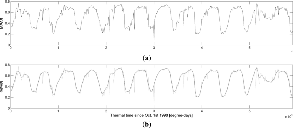
Secondly, a temporal smoothing is done with the Whittaker smoother [31–33]. Although not well-known in the remote sensing literature, according to [32] this filter has a series of advantages over the more popular and well-known Savitzky-Golay filter. Perhaps the single most important advantage is that of balancing two conflicting goals, namely preserving data fidelity and minimizing the roughness of the smoothed time series, by adjusting a single parameter λ, whose value can be set automatically using cross-validation [32]. It has been shown to perform well in remote sensing studies at sub-continental scale, notably in South America [34] and India [35]. The Whittaker smoother is here applied twice on each fAPAR time series: once with the individual fAPAR values plotted in thermal time and once using normal calendar time (using the actual dates of the fAPAR observations and not the 10-day composite dates). For each time series, λ is separately calculated. An example of the resulting smoothed time series is shown in Figure 3.
3.3.4. Extraction of fAPAR Metrics
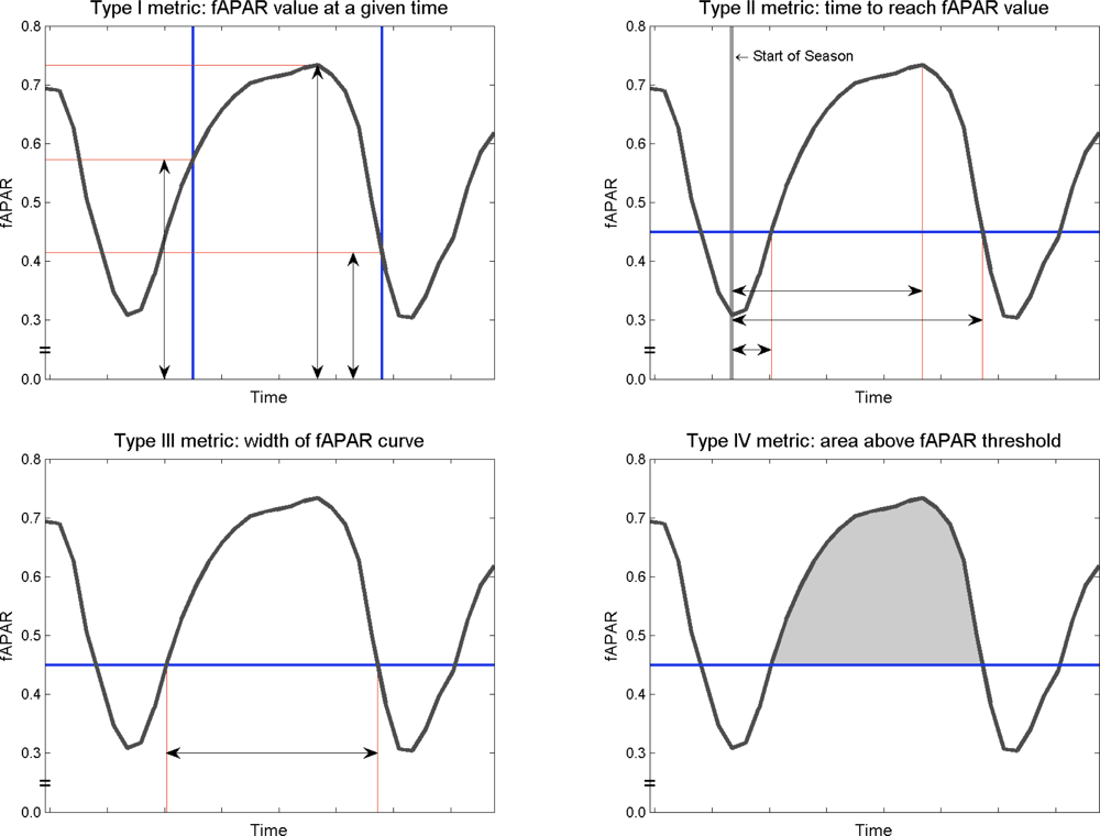
The shape of the fAPAR curve for every growing season and in every time series is characterized by a set of metrics, out of which some will then be empirically related to yield. Both kinds of series, based on calendar time and on thermal time are considered. An exploratory approach is undertaken in which a high number of various types of metrics will be generated, and later, a statistical procedure will be used to identify the relevant ones. Four different types of metrics are proposed. They are summarized in Table 1 and illustrated in Figure 4. As explained further, each metric type is defined by a series of thresholds on a given variable, referred to as the metric defining variable (MDV).
The first metric type consists of the fAPAR value at a given time. In this case, time is the MDV. For thermal time, the values of these pre-defined times range from 500 to 4,500 growing degree-days after the start of the season, which covers most of the growing season. The start of the season is considered a priori to be DoY (Day of Year) 274 of every year (corresponding to October 1 except for leap years). Times are separated by intervals of 500 growing degree days, resulting in nine time thresholds. For calendar time, nine values are similarly obtained for times ranging from 60 to 300 days after DoY 274, and are separated by 30 days intervals. These metrics will henceforth be identified as TypeI followed by ti, with i indicating the number of the threshold. The maximum value reached by the peak of fAPAR is also included as an additional metric and is labeled TypeIpeak.
The second type of metrics relates to the time (calendar or thermal time) required to reach a given fAPAR value, in either the ascending or descending phase, starting from the a priori start of the season. In this case, the MDV is fAPAR, and the threshold values used to define this type of metric go from 0.2 to 0.6 separated by 0.05 intervals, resulting in nine different metrics for the ascending phase (identified as TypeIIxxa with xx indicating the threshold) and nine metrics for the descending phase (TypeIIxxd). In addition, the time required to reach the fAPAR peak is also calculated (TypeIIpeak).
The third type of metric, which is related to the previous type, is the time separating the ascending and descending parts of the curve at a given fAPAR threshold, providing an idea of the width of the curve that is not related to the start of the season. Thresholds also range from 0.2 to 0.6 and metrics are labelled with the same nomenclature (TypeIIIxx). The final type is the area beneath the curve and above a given fAPAR threshold (again chosen from 0.2 to 0.6 and labelled TypeIVxx).
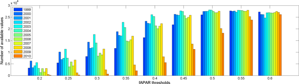
The total number of different individual metrics is 47. An important point to remark is that the same number of values will not be available for each metric. More specifically, metrics depending on fAPAR thresholds (Types II, III and IV with the exception of TypeIIpeak) are not available when the remotely-sensed estimation of fAPAR does not reach either a threshold that is too high or too low. Furthermore, as it can be seen in Figure 5, the number of available values for a given fAPAR threshold may vary from year to year. Metrics of Type I (and TypeIIpeak) always have the same number of values since there is always a fAPAR value at a given time (and there is always a maximum fAPAR).
3.4. Statistical Yield Estimation and Accuracy Assessment
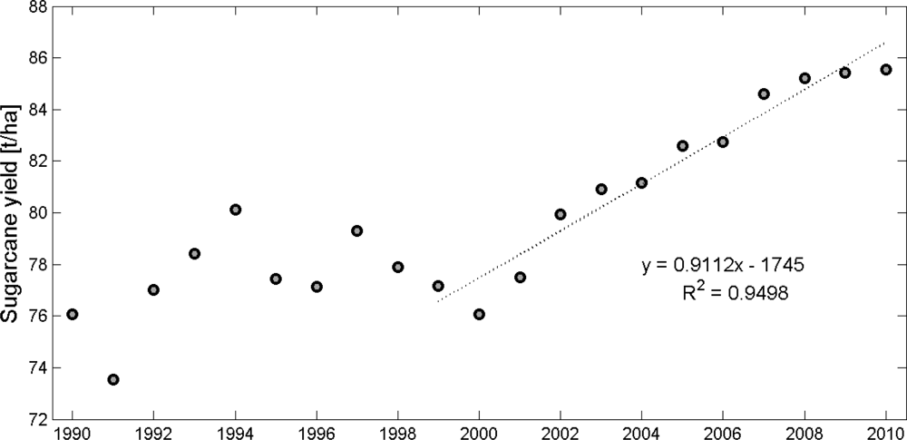
The IBGE ( www.ibge.gov.br) publishes every year statistics of total production and harvested area of the major crops at different spatial scales from country to municipality level. Therefore, official sugarcane yield can be therefore calculated as the ratio between the total production and the harvested area. The evolution of sugarcane yield in the São Paulo state during the period 1990–2010 is described in Figure 6. A significant trend drives the evolution of sugarcane yield after the period 2000–2002. In the study period (1999–2010) the yield trend is approximated by a linear function, explaining already up to 95% of the sugarcane yield variation. Several authors [16,36] explain this trend by the growing interest of sugarcane in Brazil as a source of biofuels, the increased price of energy and the fact that much newly planted sugarcane (expansion class) has higher yields in the first harvest.
When establishing a statistical relationship between the metrics and the official yield statistics, two different approaches are considered. The first one explores whether the remote sensing metrics can detect absolute changes in yield in the period studied. This may be expected, theoretically, in the areas where variations in sugarcane yield can be explained by changes in the green biomass accumulation associated to different factors: weather conditions, improvement of management practices, etc.
The second approach assumes that the yield increase over the last decade is dominated by effects that are not reflected as changes in biomass accumulation as seen by remote sensing. An example could be changes in management practices or the adoption of improved varieties that could increase substantially the yield without significant changes in the presence of green biomass visible from space. In this approach, remote sensing metrics are related statistically with the residuals of the absolute yield and the yield trend. The yield trend takes the form of a linear regression between the years (independent variable) and the absolute yield (dependent variable) adjusted by least squares methods.
For both approaches, the predictive variables are constructed based on a population of N time series selected using a crop specific spatial purity (π) threshold which ranges from 75% to 99%. If the π threshold is too harsh and reduces the time series population below N = 100, the group is discarded. For each of the 47 metrics, a predictive variable is computed, for a given year, using the median of the N values of that metric, for that year, in the selected population. A bivariate linear regression is applied on all possible pairwise combinations of the metrics (1,081 in total). A maximum of two predictive variables is used in order to avoid over-fitting. The 47 univariate regressions are also calculated to result in 1,128 possible individual regressions, out of which only those that are significantly (p-value < 0.05) related to the independent variable (either absolute yield or yield residuals) are retained. A leave-one-out cross-validation is then performed to calculate the root mean squared error (RMSE), the adjusted coefficient of determination (R2adj) and the mean sign indicator (MSI) using the following formulas:
In the formulas above, yi and ŷi are respectively observed and estimated yield (or residuals), n is the number of yield observations available and p is the number of predictive variables used (including the year for the linear trend in the case of the yield residuals). Regarding the adjusted R2, it must be noted that: (1) it can be negative; (2) its value will always be less than or equal to that of R2; and (3) unlike R2, the adjusted R2 increases only if the new term improves the model more than would be expected by chance. The MSI uses the signum function to compare how often the estimation is on the correct side of the trend. Despite its qualitative nature, this kind of information is valuable in operational crop yield forecasting, even when the absolute yield error is still considerable. MSI will have a value of 1 if all estimations and observations have the same sign, while it will be close to 0.5 when the sign correspondence is random. The calculation of MSI are not based on n, but on the subset n*, which comprises estimations that are more than 0.1 t/ha away from the trend. The rationale for this is not to count a correct or incorrect sign when the estimation is too close to the trend. The MSI is only applicable on residuals (de-trended yield).
4. Analysis of Results
4.1. Exploratory Analysis of the Remote Sensing Dataset
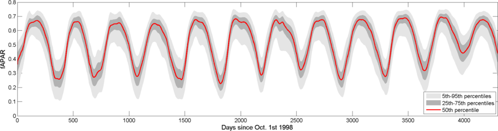
Prior to analyze the predictive capacity of the remote sensing dataset to estimate yield, an overview of the spatio-temporal information contained in it is illustrated in this section. Figure 7 provides the 5th, 25th, 50th, 75th and 95th percentiles of the ensemble of pixels with a crop specific spatial purity above or equal to 75%. These represent the overall expected behavior of sugarcane. Interestingly, during the austral winter between the last two seasons (in 2009), the biomass, as detected by the remote sensing fAPAR, did not fell as low as during the previous years, explaining why less metrics are available for the last two seasons (as seen in Figure 5). These unusually high fAPAR values observed at the end of the 2009 season are a consequence of the intense precipitation cumulated during the period between August and October 2009 in the northern half of the region, where most of the sugarcane is cultivated. According to ECMWF data it rained 270 mm for that period, which is more than twice the seasonal values (105 mm).
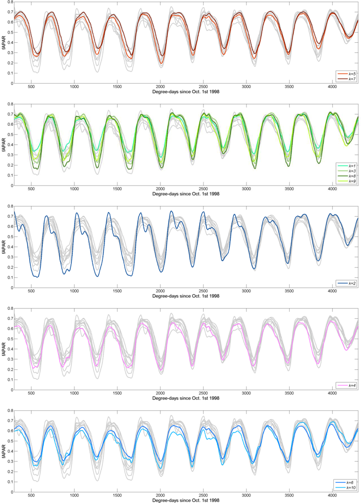
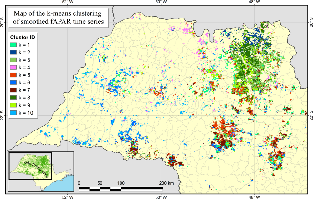
To further illustrate the spatio-temporal information contained in the dataset, the result of a k-means clustering algorithm applied to all (thermal) time series with π ≥ 75% is illustrated in Figure 8. A strong spatial structure is apparent. Clusters 3, 8 and 9 are mostly located in the North-Eastern part of the state, where the landscape is dominated by sugarcane and the climate is tropical savannah (Af), whereas clusters 5 and 7 are mostly located in the Southern part characterized by the humid subtropical climate (Cfa). Clusters 4, 6 and 10 generally seem to attain lower fAPAR values than the rest (as shown on the profiles in Figure 9) and seem to be in distinctively different geographic regions: Cluster 4 in the center North while the other two in the scattered points in the Western part of the state. Cluster 2, located almost exclusively in the northernmost part of the state, displays a particular bi-modal temporal profile in the beginning of the study period. This cluster comprises the municipalities of Ipua and, mainly, Miguelopolis, where sugarcane acreage multiplied by three from 2000 to 2007 according to the IBGE. Therefore, the first mode that can be observed in the seasonal fAPAR curve from 2000 to 2006 is reproducing the phenological cycle of summer cereals (maize and soybean). After 2007, the gradual replacement of these crops by sugarcane results in fAPAR profiles closer to those expected from sugarcane.
4.2. Performance of Remote Sensing Indicators to Estimate Sugarcane Yield
The performance of sugarcane yield estimations for the entire state of São Paulo is resumed in Figure 10 for the four types of analyses: with or without the time trend component and using either thermal or calendar time. The figure presents the evolution of the 3 indicators, RMSE, R2adj and MSI, when increasing thresholds of spatial purity are used to select the population of time series from which to estimate the yield. For each time series population with increasing π thresholds, the metric or metrics having the smallest RMSE (and with a p-value > 0.05) are listed in Table 2.
The analysis based on absolute yield indicates that a considerable part of its variability during the study period is detectable by remote sensing. The results further show there is an influence of time series purity on the accuracy of the estimations. This influence is stronger for the analysis based on thermal time, which provides worst results than calendar time up to around π thresholds of 90%, after which accuracy increases considerably, showing better performances than calendar time with respect to RMSE. For the higher purities, both thermal and calendar time analyses can explain almost as much variance as the trend, as shown by the R2adj values higher than 0.8. While the corresponding RMSE of around 1.5 t/ha still appears considerably higher than that of the trend (0.78 t/ha) in absolute value, if it is compared to the average state yield it represents less than 2% of error.
As shown in Table 2, the types of metrics responsible for this performance are different whether thermal or calendar time is used. This can be expected due to the fact that time series in the thermal time axis are partially normalized according to sugarcane phenology, while those in calendar time can be shifted from one season to another if the some parts of the season were warmer or colder. As a consequence, metrics describing the timing of events (such as TypeI or TypeII) are, a priori, more explicative of yield when using calendar time, while metrics describing the length to the season (such as TypeIII) are expected to be more reliable using thermal time. This is actually what can be observed in Table 2. Another remark is that the selected metrics change along the pixel purity dimension. This suggests that some metrics, in order to explain yield variations, require a minimum purity (i.e., less signal contamination can be tolerated), while other are more robust and can be applied on more mixed pixels (but with potentially less explicative power). This also changes with respect to thermal and calendar time: a combination of TypeIId with TypeIV is effectively the best for thermal time and not for calendar time up to a certain value, after which the opposite is observed.
Beyond detecting the absolute changes in the sugarcane yield in São Paulo, the analysis based on the yield residues indicates that remote sensing fAPAR metrics are also sensitive to the inter-annual yield variability. Taking the trend into account improves the yield forecasting performance to reach an RMSE of around 0.6 t/ha that doesn’t vary much with respect to the π threshold used, and which remains consistently below the RMSE using trend only. In this case, thermal time out-performs calendar time for almost all π thresholds and for all three performance indicators. The MSI illustrates how, in most cases (around 90% when using thermal time), it is possible to predict based on the metrics whether the yield will be above or below the trend.
The metrics providing the best performances also change with respect to the time definition that is employed. For thermal time, a long part of the purity spectrum is covered by a combination of TypeIIa and TypeIII metrics, while the TypeIV metrics are also often present. For calendar time, the use of the TypeIV metric type is dominant, and it always involves very low fAPAR cutting thresholds (fAPAR = 0.2 or fAPAR = 0.25). This may have undesirable consequences since, as illustrated in Figure 5, the remotely-sensed estimation of fAPAR seldom reaches these low thresholds, and this number varies considerably from year to year (e.g., for 2009 and 2010 there are very little pixels available, explained by the fact that the minimum fAPAR values reached between these two seasons is much higher than what it usually is, as seen on Figure 7).
4.3. Timing of Yield Estimation
In crop yield forecasting, there is not only a strong interest on the absolute predictive capacity but also on how early this prediction can be made. By construction, the metrics proposed in this study are not available at the same time. Some metrics beneficiate from exploiting as much information as they can from the time series to explain yield variability (which explains why TypeIV with low fAPAR threshold are selected quite often in Table 2), but as a consequence they are only available later in the season (sometimes practically at harvest time). A compromise may be desirable in order to trade-off accuracy for timeliness. On the other hand, early estimations are only valid under the assumption that the remaining of the season follows a normal trajectory, thus limiting how much trade-off can be made.
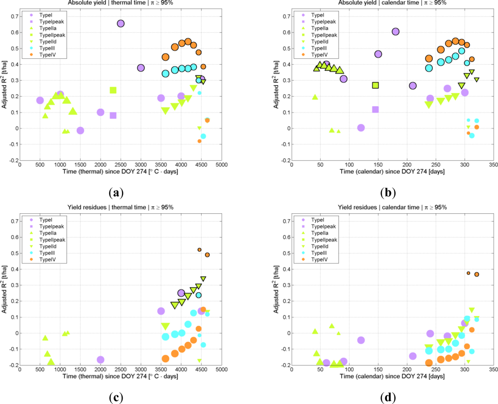
In order to illustrate the predictive capacity of each individual metric with respect to time, Figure 11 plots the value of the R2adj at the time at which it is effectively available (the average time over the 12 years is considered here).
For graphical simplicity, only univariate regressions with either absolute yield or residues are considered, and only metrics obtained from the purer time series are used (extracted with π ≥ 95%). It is worth noting how, when the analysis is based on absolute yield instead of yield residues, metrics of the same type behave differently when their fAPAR thresholds increase. For the residues, there is an expected behavior that later metrics (involving lower fAPAR thresholds and thus, potentially finer information) have higher explanatory power, as indicated by the R2adj. For absolute yield, the performance of the metrics can deteriorate for lower (and thus later) fAPAR thresholds after an optimal performance. The order of performance of the metrics is also different: for the residues, TypeIId perform better than TypeIII, and TypeIII better than TypeIV; for the absolute yield TypeIV performs best, then TypeIII and only after that comes TypeIId. This pattern is similar for thermal and calendar time. TypeI metrics, which do not depend on fAPAR thresholds, generally provide better performance later in the season in the residues analysis, but for estimating absolute yield, they provide a much stronger explanatory capacity shortly after the peak of fAPAR. Figure 11 also contains information on the reliability of the regressions by way of indicating the metrics for with the p-value is below 0.05. As expected, metrics significantly related to yield tend to appear later in the season. But the behavior for the calendar time analysis is particular in that there are many significant metrics for absolute yield throughout the season, but only very few for the residues. Furthermore, as mentioned before, the metrics for this latter analysis are almost exclusively based on very low TypeIV metrics, for which there are less samples and they arrive late in the season. Overall this suggests that forecasting the residues with calendar time is not optimal.
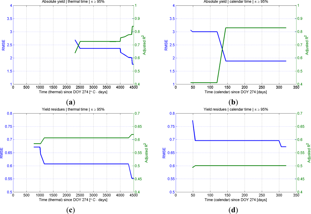
As mentioned before, Figure 11 only presents results from univariate regressions. Since the best performances are generally obtained using a bivariate regression (as seen in Table 2), the issue of timing for these cases is also included in Figure 12, where the performance of the best available (and significant) set of metrics is plotted against its timeliness. The example shown (for π ≥ 95%) illustrate how, for the yield residues based on thermal time, it may not be worthwhile to use the best set of metrics since they are only available very late in the season and provide only a marginal increase in performance, while a decent estimation is already available much earlier. In the case of absolute yield estimated with calendar time, the best set of metrics is already available quite early in the season.
5. Discussion
The results demonstrate that low resolution remote sensing time series reflect valuable information on the dynamics of sugarcane in the state of São Paulo. SPOT-VEGETATION 1 km fAPAR data not only reveals a strong spatio-temporal structure, as shown by the clustering exercise, but it is also sensitive enough to detect both absolute changes in green biomass accumulation and changes in its inter-annual variability. This is shown respectively by the yield estimation accuracy of around 1.5 t/ha (or 2%) without considering the trend, and about 0.6 t/ha when the trend is taken into account. Despite the fact that the trend captures already most of yield variability, and using it for forecasting provides better results, being able to make accurate predictions based on the signal without requiring modeling the trend is encouraging. Such approach could work despite changes in the shape of the trend. In São Paulo region, for instance, it is unlikely that a linear trend with the same slope will remain valid for the years to come because the rate of yield increase will probably change, with a potential slow down as less area of new expansion sugarcane (which typically has higher yields) becomes available, but also a potential increase as different yield-improving techniques become available [16]. Moreover, this suggests that monitoring sugarcane with satellite remote sensing in regions where crop statistics are inexistent or unreliable could provide meaningful qualitative information about yield, regardless of possible trends in crop production.
The fact that the metrics that stand out as most significant are different when either absolute yield or residues are used as the dependent variable indicates that the remote sensing signal carries various different types of information. In that respect, this study provides a methodological framework to select the most appropriate metrics without any a priori assumptions regarding their nature. Indeed, the various metrics of different types are constructed systematically, with the equally systematic statistical exploration of their relationship with yield, and how this relationship holds along the season and for different spatial purities. This methodological framework could be transferable to other crops in different agro-ecosystems to improve crop yield forecasting systems and agricultural monitoring in general. It must be noted, however, that the good results obtained in this study are also attributable to the fact that sugarcane yield is related to the presence of green biomass, which itself is directly linked to fAPAR. By contrast, in cereals the yield is partially determined by weather during grain formation and maturity phases, and is therefore less dependent on the development of green leaf area, which makes the relationship between fAPAR and yield less straightforward. Furthermore, the tropical climate of the study area is probably more stable and predictable than the temperate climate of higher latitudes, making it easier to model inter-annual yield deviations from the trend since extreme events with unpredictable effects are rarer.
An originality of this study is to explore the use of thermal time versus calendar time for retrieving information from the remote sensing time series. As mentioned before, the use of thermal time allows a partial normalization of the time series with respect to phenology. By doing so, the confounding effects of growth and phenological development on the fAPAR observations can be partially separated. The result allows comparing directly information from one year to another, and across large geographic extents in which strong climate gradients can be encountered. Metrics based on thermal time may be more sensitive to effects of drought on biomass at a given critical crop stage, for instance, while trying to detect this using calendar time is hampered if some seasons are in advance or in delay with respect to the mean, due to inter-annual variations of the temperature regime. Such advantage could be even more pertinent in other climates where the day to day temperature oscillations are larger. The reason why the normalization is only considered partial is that the plant phenology is not exclusively related to temperature. Other biotic and abiotic stresses, which are not taken into account here, can hamper development. Furthermore, the characterization of thermal time adopted here is a coarse simplification of the reality based only on attributing a uniform weight to all temperatures above Tb. A more realistic approach would use a curvilinear model, bounded by a minimum and maximum temperature and with a higher weight to the optimum temperature for the crop of interest [37,38]. Ideally, thermal time should be replaced by photo-thermal time, in which the integration of temperature with time is restricted to the duration of the light period and calculated on an hourly basis [29]. However, a thorough understanding of the utility and limitations of the thermal time concept (as provided in [27,28]) is necessary to judge whether increasing the complexity of the calculations provides an added-value given the assumptions that must be made in the present context.
Despite the advantages of thermal time, it adds an extra level of complexity to the analysis. This study indicates that it is worthwhile to take this step in the case when the inter-annual variability of the yield residues is explored, where the estimation based on thermal time clearly outperforms the one using calendar time. The latter not only results in larger RMSE, but also has fewer metrics significantly related to yield residues, and those metrics who are (TypeIV20 or TypeIV25) arrive late in season and can only be available for a limited amount of time series, jeopardizing the spatial representativity of the sampling set. For estimating absolute yield, however, having the analysis based on simple calendar time generally results in similar or better results than using the more complicated thermal time. Furthermore, the metrics responsible for this higher performance are generally available earlier in the season than with thermal time, making them even more interesting in a crop yield forecasting context. An important remark is that, unlike most studies, the calendar time analysis is based on the actual day of observation instead of a fixed date imposed by the compositing scheme of the remote sensing data. This difference may have affected positively the high performance of the absolute yield estimation.
Although estimating absolute yield based on thermal time does not out-perform the analysis based on calendar time, some points indicate it can be considered as valid alternative to the use of calendar time. The increase in performance of absolute yield estimation with thermal time is more sensitive to purer time series than when using calendar time. This suggests that having a signal that is more specific to sugarcane does not bring more explanatory power to metrics based on calendar time, but it does for metrics based on thermal time. This higher dependency on crop specific purity is expected because the calculation of thermal time is based on a base temperature which is crop specific. The fact that a more complex analysis, which attempts to be closer to the crop, is rewarded by better explanatory power is encouraging for developing further research in that direction. Perhaps an interesting approach for yield estimation could be combining both metric types (based either on thermal and calendar time) together to provide complementary information and enhanced forecasting skills. In such hybrid approach, the calendar time metrics could come from an ensemble of time series with relatively low pixel purity in order to have a large spatial distribution of samples, while the thermal time metrics could be extracted from a subset of purer time series to provide finer information that is closer to plant physiology.
The selection of appropriate time series, based on the Canasat maps and the concept of crop specific pixel purity, had a tangible effect on the quality of the yield estimations realized in this study. However, the Canasat maps were used only to identify the general potential area where sugarcane is likely to be found in São Paulo, including all area that has been part of the four Canasat classes in any of the years within the period 1999–2011. This approach had the advantage of being simple. It also enabled the confirmation that the fAPAR time series did react to the changes from different land uses towards sugarcane. However, it implies that sometimes fAPAR metrics were not describing exclusively sugarcane areas, and that may have undermined the quality of the yield estimation, complicating the interpretation of the crop specific pixel purity. Given the high quality of the Canasat data, a refinement of the approach should be pursued to provide a finer yield forecast by cleaning the multiannual fAPAR metrics dataset already constructed. The various Canasat maps should be used to remove all metrics related to non-sugarcane, namely those corresponding to places classified as under renovation during a given year and all metrics corresponding to a time and place where the class expansion is present in a subsequent year. Then, the remaining metrics could be analyzed based on the three categories of sugarcane, potentially showing a sensitivity of the remote sensing signal to the decrease in yield expected respectively in the categories expansion, renovated and ratoon. The characterization of the spatial response function of the remote sensing instrument could also be improved, but it is probably sufficient as it is for SPOT-VEGETATION, which is a push-broom sensor. Applying the methodology presented here on MODIS data could be promising; given it has a spatial resolution which is four times finer, and already has a data archive which is long enough (since 2000). Some recent work is already exploring a similar approach on sugarcane by integrating time on MODIS NDVI data [39]. However, MODIS is a whisk-broom sensor for which the observation footprint varies strongly according to the scan angle [40–42], requiring a more elaborate model of the spatial response in order to use the daily data as it is required in this paper.
Another discussion point is that the accuracy of the methods presented has a general dependence on the reliability of official statistics which fAPAR metrics are related to. In Brazil, the private sector also reports regional yield estimations under the umbrella of the União da Indústria de Cana-de-Açúcar (UNICA). This may be an alternative and independent source of information which could be used to further validate and consolidate the present results.
Based on this work, various paths for further improvements and research can be followed. A logical continuation would be to explore the possibility of near-real time forecasting at the regional level with the datasets used in this study. This could also be done based on the biophysical products that will be available from the future Copernicus services, the European Earth observation program. These will composed of the BioPar pre-operational chains designed under the Geoland2 project, and for which the version 2 is designed to work in near-real time conditions [43]. Another potential perspective is to downscale the approach to see the predictive capacity of remote sensing information at the municipality level, for which official yield statistics are also available. At that scale, the statistical relationship between fAPAR metrics and yield could be reasoned differently to limit over-parameterisation problem, by either fixing the slope or intercept regression coefficients per municipality, as investigated in [44]. The clustering exercise done in this study also remained underexploited. The relation between the average metrics per cluster with state yield could be explored, as perhaps some cluster covering the main production zones have a more stable relationship with state-level yield. To avoid the dependency of the method to a pre-established sugarcane map, a classification exercise should be envisaged based on the Canasat maps, in order to see how the fAPAR dataset can accurately identify sugarcane from other land covers, and perhaps even identify the type of sugarcane it is, and thus perhaps detect yield differences between sugarcane types. Further improvements could include adapting the approach to other satellite remote sensing instruments with higher spatial resolution, and exploring its applicability to other crops in other climates.
6. Conclusions
The proposed post-processing of the Fraction of Absorbed Photosynthetically Active Radiation (fAPAR) time series enables to provide metrics that can be used to accurately estimate sugarcane yield over the state of São Paulo. The dataset has a strong spatio-temporal structure and is sensitive both to absolute changes in biomass accumulation and changes in its inter-annual variability. The capacity of estimating yield based on this dataset was shown to be influenced by various aspects, namely: (1) the way time is regarded (thermal or calendar); (2) the purity of the signal; (3) how the information is extracted from the time series (i.e., the type of metrics); and (4) the timing of when the information is available. Concerning what type of metrics to use in the case of São Paulo, the recommendations that emerge from this study are that TypeIII metrics (representing the observed length of the growing season) are to be preferred for thermal time, but they should be combined with another metric providing complementary information on the position in time of the curve, such as with metric TypeIt5 or TypeII55a. When using calendar time, either TypeIId (decrease of the curve) or TypeIV (area under the curve) provide a better relation to yield. Yet for both cases (thermal and calendar), the best metrics may change considerably depending on how pure the pixel is. Regarding timeliness, it appears yield estimations based on metrics obtained a little after the peak of fAPAR can be done without seriously compromising performance. Since the remote sensing product used in this study is very similar to that which will be provided by Copernicus, the European Earth observation program (previously known as GMES or Global Monitoring for Environment and Security), it is expected that the conclusions obtained here will remain valid for the future Copernicus data.
Acknowledgments
The authors thank the Canasat Project for providing the shapefiles of their maps which greatly contributed in improving the present analysis. The authors equally thank the four anonymous reviewer for their contribution in improving the quality of the manuscript.
References
- Atzberger, C. Advances in remote sensing of agriculture: Context description, existing operational monitoring systems and major information needs. Remote Sens 2013, 5, 949–981. [Google Scholar]
- Rembold, F.; Atzberger, C.; Rojas, O.; Savin, I. Using low resolution satellite imagery for yield prediction and yield anomaly detection. Remote Sens. 2013. under review. [Google Scholar]
- Galvão, L.S.; Formaggio, A.R.; Tisot, D.A. Discrimination of sugarcane varieties in Southeastern Brazil with EO-1 Hyperion data. Remote Sens. Environ 2005, 94, 523–534. [Google Scholar]
- Fortes, C.; Demattê, J.A.M. Discrimination of sugarcane varieties using Landsat 7 ETM+ spectral data. Int. J. Remote Sens 2006, 27, 1395–1412. [Google Scholar]
- Rudorff, B.F.T.; De Aguiar, D.A.; Da Silva, W.F.; Sugawara, L.M.; Adami, M.; Moreira, M.A. Studies on the rapid expansion of sugarcane for ethanol production in São Paulo State (Brazil) using Landsat data. Remote Sens 2010, 2, 1057–1076. [Google Scholar]
- Romani, L.A.S.; Goncalves, R.R.V.; Amaral, B.F.; Chino, D.Y.T.; Zullo, J.; Traina, C.; Sousa, E.P.M.; Traina, A.J.M. Clustering Analysis Applied to NDVI/NOAA Multitemporal Images to Improve the Monitoring Process of Sugarcane Crops. Proceedings of the 6th International Workshop on the Analysis of Multi-temporal Remote Sensing Images (Multi-Temp), Trento, Italy, 12–14 July 2011; pp. 33–36.
- Xavier, A.C.; Rudorff, B.F.T.; Shimabukuro, Y.E.; Berka, L.M.S.; Moreira, M.A. Multi-temporal analysis of MODIS data to classify sugarcane crop. Int. J. Remote Sens 2006, 27, 755–768. [Google Scholar]
- de Aguiar, D.A.; Rudorff, B.F.T.; Adami, M.; Shimabukuro, Y.E. Imagens de sensoriamento remoto no monitoramento da colheita da cana-de-açúcar. Engenharia Agrícola 2009, 29, 440–451. [Google Scholar]
- Mobasheri, M.R.; Chahardoli, M.; Farajzadeh, M. Introducing PASAVI and PANDVI methods for sugarcane physiological date estimation, using ASTER images. J. Agr. Sci. Tech 2010, 12, 309–320. [Google Scholar]
- Gonçalves, R.R.V.; Zullo, J.; Romani, L.A.S.; Nascimento, C.R.; Traina, A.J.M. Analysis of NDVI time series using cross-correlation and forecasting methods for monitoring sugarcane fields in Brazil. Int. J. Remote Sens 2012, 33, 4653–4672. [Google Scholar]
- Almeida, T.I.R.; De Souza Filho, C.R.; Rossetto, R. ASTER and Landsat ETM+ images applied to sugarcane yield forecast. Int. J. Remote Sens 2006, 27, 4057–4069. [Google Scholar]
- Picoli, M.C.A.; Rudorff, B.F.T.; Rizzi, R.; Giarolla, A. Índice de vegetação do sensor MODIS na estimativa da produtividade agrícola da cana-de-açúcar. Bragantia 2009, 68, 789–795. [Google Scholar]
- Lofton, J.; Tubana, B.S.; Kanke, Y.; Teboh, J.; Viator, H.; Dalen, M. Estimating sugarcane yield potential using an in-season determination of normalized difference vegetative index. Sensors 2012, 12, 7529–7547. [Google Scholar]
- Bégué, A.; Todoroff, P.; Pater, J. Multi-time scale analysis of sugarcane within-field variability: improved crop diagnosis using satellite time series? Precision Agr 2008, 9, 161–171. [Google Scholar]
- Fernandes, J.L.; Rocha, J.V.; Lamparelli, R.A.C. Sugarcane yield estimates using time series analysis of spot vegetation images. Sci. Agr 2011, 68, 139–146. [Google Scholar]
- Cheavegatti-Gianotto, A.; De Abreu, H.M.C.; Arruda, P.; Bespalhok Filho, J.C.; Burnquist, W.L.; Creste, S.; Di Ciero, L.; Ferro, J.A.; De Oliveira Figueira, A.V.; De Sousa Filgueiras, T.; et al. Sugarcane (Saccharum X officinarum): A reference study for the regulation of genetically modified cultivars in Brazil. Trop. Plant Biol 2011, 4, 62–89. [Google Scholar]
- Mello, M.; Adami, M.; Rudorff, B.; Aguiar, D. Canasat Project Accuracy Assessment of Sugarcane Thematic Maps. Proceeding of the 10th International Symposium on Spatial Accuracy Assessment in Natural Resources and Environmental Sciences, Florianopolis, Brazil, 10–13 July 2012; pp. 281–286.
- Weiss, M.; Baret, F.; Eerens, H.; Swinnen, E. FAPAR over Europe for the Past 29 Years: A Temporally Consistent Product Derived from AVHRR and VEGETATION Sensor. Proceeding of the third RAQRS Workshop, Valencia, Spain, 27 September–1 October 2010; pp. 428–433.
- Baret, F.; Hagolle, O.; Geiger, B.; Bicheron, P.; Miras, B.; Huc, M.; Berthelot, B.; Nino, F.; Weiss, M.; Samain, O.; et al. LAI, fAPAR and fCover CYCLOPES global products derived from VEGETATION: Part 1: Principles of the algorithm. Remote Sens. Environ 2007, 110, 275–286. [Google Scholar]
- Baruth, B.; Royer, A.; Klisch, A.; Genovese, G. The use of remote sensing within the MARS crop yield monitoring system of the European Commission. Int. Arch. Photogramm. Rem. Sens. Spat. Inform. Sci 2008, 37, 935–940. [Google Scholar]
- Holben, B.N. Characteristics of maximum-value composite images from temporal AVHRR data. Int. J. Remote Sens 1986, 7, 1417–1434. [Google Scholar]
- Cracknell, A.P. Synergy in remote sensing–What’s in a pixel? Int. J. Remote Sens 1998, 19, 2025–2047. [Google Scholar]
- Duveiller, G.; Defourny, P. A conceptual framework to define the spatial resolution requirements for agricultural monitoring using remote sensing. Remote Sens. Environ 2010, 114, 2637–2650. [Google Scholar]
- Duveiller, G.; Baret, F.; Defourny, P. Crop specific green area index retrieval from MODIS data at regional scale by controlling pixel-target adequacy. Remote Sens. Environ 2011, 115, 2686–2701. [Google Scholar]
- Duveiller, G.; Baret, F.; Defourny, P. Using thermal time and pixel purity for enhancing biophysical variable time series: an inter-product comparison. IEEE Trans. Geosci. Remote Sens. 2013. in press. [Google Scholar]
- Réaumur, R.A. Observations du thermomètre faites pendant l’année MDCCXXXV comparées à celles qui ont été faites sous la ligne à Isle-de-France, à Alger et en quelques-unes de nos Isles de l’Amérique. Mémoires de l’Académie Royale des Sciences 1735, 545–576. [Google Scholar]
- Bonhomme, R. Bases and limits to using ‘degree.day’ units. Eur. J. Agron 2000, 13, 1–10. [Google Scholar]
- Trudgill, D.L.; Honek, A.; Li, D.; Van Straalen, N.M. Thermal time—Concepts and utility. Ann. Appl. Biol 2005, 146, 1–14. [Google Scholar]
- Purcell, L.C. Comparison of thermal units derived from daily and hourly temperatures. Crop Sci 2003, 43, 1874–1879. [Google Scholar]
- Atwell, B.J.; Kriedemann, P.E.; Turnbull, C.G.N. Plants in Action: Adaptation in Nature, Performance in Cultivation; Palgrave MacMillan: Sydney, NSW, Australia, 1999. [Google Scholar]
- Whittaker, E.T. On a new method of graduation. Proc. Edinb. Math. Soc 1923, 41, 63–75. [Google Scholar]
- Eilers, P.H.C. A perfect smoother. Anal. Chem 2003, 75, 3631–3636. [Google Scholar]
- Atzberger, C.; Eilers, P.H.C. Evaluating the effectiveness of smoothing algorithms in the absence of ground reference measurements. Inter. J. Remote Sens 2011, 32, 3689–3709. [Google Scholar]
- Atzberger, C.; Eilers, P.H.C. A time series for monitoring vegetation activity and phenology at 10-daily time steps covering large parts of South America. Int. J. Digit. Earth 2011, 4, 365–386. [Google Scholar]
- Atkinson, P.M.; Jeganathan, C.; Dash, J.; Atzberger, C. Inter-comparison of four models for smoothing satellite sensor time-series data to estimate vegetation phenology. Remote Sens. Environ 2012, 123, 400–417. [Google Scholar]
- Marin, F.R.; Carvalho, G.L. de Spatio-temporal variability of sugarcane yield efficiency in the state of São Paulo, Brazil. Pesqui. Agropecu. Bras 2012, 47, 149–156. [Google Scholar]
- Yin, X.; Kropff, M.J.; McLaren, G.; Visperas, R.M. A nonlinear model for crop development as a function of temperature. Agr. Forest Meteorol 1995, 77, 1–16. [Google Scholar]
- Yan, W.; Hunt, L.A. An equation for modelling the temperature response of plants using only the cardinal temperatures. Ann. Bot 1999, 84, 607–614. [Google Scholar]
- Mulianga, B.; Begue, A.; Simoes, M.; Todoroff, P. Forecasting regional sugarcane yield based on time integral and spatial aggregation of MODIS NDVI. Remote Sens. 2013. under review. [Google Scholar]
- Wolfe, R.E.; Roy, D.P.; Vermote, E. MODIS land data storage, gridding, and compositing methodology: Level 2 grid. IEEE Trans. Geosci. Remote Sens 1998, 36, 1324–1338. [Google Scholar]
- Tan, B.; Woodcock, C.E.; Hu, J.; Zhang, P.; Ozdogan, M.; Huang, D.; Yang, W.; Knyazikhin, Y.; Myneni, R.B. The impact of gridding artifacts on the local spatial properties of MODIS data: Implications for validation, compositing, and band-to-band registration across resolutions. Remote Sens. Environ 2006, 105, 98–114. [Google Scholar]
- Duveiller, G. Caveats in calculating crop specific pixel purity for agricultural monitoring using MODIS time series. Proc. SPIE 2012, 8531, 85310J–1. [Google Scholar]
- Baret, F.; Weiss, M.; Verger, A.; Kandasamy, S. BioPar Methods Compendium LAI, FAPAR and FCOVER from VEGETATION P Product Series. Geoland 2-Towards an Operational GMES Land Monitoring Core Service. g2-BP-RP-BP038. Version 3.0, Geoland2 Consortium. 2012. [Google Scholar]
- Meroni, M.; Marinho, E.; Sghaier, N.; Verstrate, M.; Leo, O. Remote sensing based yield estimation in a stochastic framework—Case study of durum wheat in Tunisia. Remote Sens 2013, 5, 539–557. [Google Scholar]


| Type | Description | Metric Defining Variable (MDV) | Thresholds of MDV [min:interval:max] | Max. Potential Number of Metrics |
|---|---|---|---|---|
| I | Value of fAPAR at a given time | Time* | 60:30:300 (time) or 500:500:4500 (th. time), peak | 10 |
| II | Time at which a given fAPAR value is reached in either the ascending or descending phase | fAPAR | 0.2:0.05:0.6, peak | 19 |
| III | Time separating the ascending and descending parts of the curve at a given fAPAR threshold | fAPAR | 0.2:0.05:0.6 | 9 |
| IV | Area above a given fAPAR threshold | fAPAR | 0.2:0.05:0.6 | 9 |
*Calculated in either days or growing degree-days after DoY 274 of each year.
| Absolute Yield | Yield Residuals | |||||||
|---|---|---|---|---|---|---|---|---|
| Time | Thermal | Calendar | Thermal | Calendar | ||||
| π | X1 | X2 | X1 | X2 | X1 | X2 | X1 | X2 |
| 75 | II60d | IV50 | It4 | It2 | II30d | II20d | II40a | IV20 |
| 76 | II60d | IV50 | It4 | It2 | II30d | II20d | II40a | IV20 |
| 77 | II60d | IV50 | It4 | It2 | IV25 | II40a | IV20 | |
| 78 | II60d | IV50 | It4 | It2 | IV25 | II40a | IV20 | |
| 79 | II60d | IV50 | It4 | It2 | IV25 | IV20 | ||
| 80 | II60d | IV50 | It4 | It2 | IV25 | IV20 | ||
| 81 | II60d | IV50 | It4 | It2 | IV25 | IV20 | ||
| 82 | It5 | III40 | II45d | IV35 | IV25 | IV20 | ||
| 83 | II35d | III25 | II45d | IV35 | IV25 | IV20 | ||
| 84 | II35d | III25 | II45d | IV35 | IV25 | IV20 | ||
| 85 | IV30 | III25 | II45d | IV35 | II55a | III40 | IV20 | |
| 86 | IV30 | III25 | II45d | IV35 | II55a | III40 | IV20 | |
| 87 | IV30 | III25 | II45d | IV35 | II55a | III40 | IV20 | |
| 88 | It5 | III40 | II45d | IV35 | II55a | III40 | IV20 | |
| 89 | It5 | III40 | II45d | IV35 | II55a | III40 | IV20 | |
| 90 | It5 | III40 | II45d | IV35 | II55a | III40 | IV20 | |
| 91 | It5 | III40 | II45d | IV35 | II55a | III35 | IV20 | |
| 92 | It5 | III40 | II45d | IV35 | II55a | III35 | IV20 | |
| 93 | II35d | III20 | It2 | IIpeak | II55a | III35 | IV20 | |
| 94 | III35 | III20 | It2 | IIpeak | II55a | III35 | IV25 | |
| 95 | II35d | III20 | It2 | IIpeak | II55a | III35 | IV20 | |
| 96 | III35 | III20 | It5 | It2 | II55a | II30a | II40a | II35a |
| 97 | It5 | III35 | It5 | It2 | II50a | II30a | II40a | II35a |
| 98 | II35d | III20 | II55d | IV40 | IV20 | II40a | II35a | |
| 99 | It5 | III40 | II55d | IV40 | IV20 | II45a | II30a | |
Share and Cite
Duveiller, G.; López-Lozano, R.; Baruth, B. Enhanced Processing of 1-km Spatial Resolution fAPAR Time Series for Sugarcane Yield Forecasting and Monitoring. Remote Sens. 2013, 5, 1091-1116. https://doi.org/10.3390/rs5031091
Duveiller G, López-Lozano R, Baruth B. Enhanced Processing of 1-km Spatial Resolution fAPAR Time Series for Sugarcane Yield Forecasting and Monitoring. Remote Sensing. 2013; 5(3):1091-1116. https://doi.org/10.3390/rs5031091
Chicago/Turabian StyleDuveiller, Grégory, Raúl López-Lozano, and Bettina Baruth. 2013. "Enhanced Processing of 1-km Spatial Resolution fAPAR Time Series for Sugarcane Yield Forecasting and Monitoring" Remote Sensing 5, no. 3: 1091-1116. https://doi.org/10.3390/rs5031091