Article

Use of Landsat and SRTM Data to Detect Broad-Scale Biodiversity Patterns in Northwestern Amazonia

1
Department of Global Ecology, Carnegie Institution for Science, Stanford, CA 94305, USA
2
Facultad de Ciencias Biológicas, Universidad Nacional de la Amazonía Peruana, Iquitos, Peru
3
Department of Biology, University of Turku, FI-20100 Turku, Finland
4
Center for Conservation Education and Sustainability, Smithsonian Conservation Biology Institute, National Zoological Park, Washington, DC 20013, USA
*
Author to whom correspondence should be addressed.
Remote Sens. 2012, 4(8), 2401-2418; https://doi.org/10.3390/rs4082401
Submission received: 20 June 2012 / Revised: 10 August 2012 / Accepted: 10 August 2012 / Published: 15 August 2012
(This article belongs to the Special Issue Remote Sensing of Biological Diversity)

Abstract

:
Vegetation maps are the starting point for the design of protected areas and regional conservation plans. Accurate vegetation maps are missing for much of Amazonia, preventing the development of effective and compelling conservation strategies. Here we used a network of 160 inventories across northwestern Amazonia to evaluate the use of Landsat and Shuttle Radar Topography Mission (SRTM) data to identify floristic and edaphic patterns in Amazonian forests. We first calculated the strength of the relationship between these remotely-sensed data, and edaphic and floristic patterns in these forests, and asked how sensitive these results are to image processing and enhancement. We additionally asked if SRTM data can be used to model patterns in plant species composition in our study areas. We find that variations in Landsat and SRTM data are strongly correlated with variations in soils and plant species composition, and that these patterns can be mapped solely on the basis of SRTM data over limited areas. Using these data, we furthermore identified widespread patch-matrix floristic patterns across northwestern Amazonia, with implications for conservation planning and study. Our findings provide further evidence that Landsat and SRTM data can provide a cost-effective means for mapping these forests, and we recommend that maps generated from a combination of remotely-sensed and field data be used as the basis for conservation prioritization and planning in these vast and remote forests.

Graphical Abstract

1. Introduction

Vegetation maps are important tools for the study and conservation of ecological systems [1]. Accurate and detailed vegetation maps [2] are lacking for much of Amazonia, however, due to the sheer size of the area to be surveyed, the inaccessibility of these forests, and limited funding, amongst other factors. As a result, studies of broad-scale patterns in Amazonia have often depended upon relatively small networks of widely distributed field plots [36]. Recent findings suggest that these datasets may fail to capture widespread but unsampled patterns, including extensive floristic and edaphic discontinuities, illustrating the need for improved survey in these vast and remote forests [2,711].
Remotely-sensed data, and particularly Landsat imagery and Shuttle Radar Topography Mission (SRTM) digital elevation data, offer a solution to many of these challenges. Landsat and SRTM data are accessible without charge, cover large areas with single datasets, and offer global coverage [12,13]. Patterns in Landsat data, furthermore, are known to correspond to floristic patterns in Amazonian forests [1421]; and patterns in SRTM data can be used to infer geological patterns [8,22]. Given the relationship between geological and floristic patterns in Amazonian forests, SRTM data might therefore be used to support and possibly infer floristic patterns [8,15]. As such, combining satellite imagery with field inventory offers the possibility of mapping large expanses of Amazonian forests with a modest investment of time, personnel, and funding [8,15,16].
Although a number of studies have quantified the relationship between remotely-sensed data and plant species composition in Amazonia [1519], these studies are relatively few compared to the use of Landsat data for mapping deforestation or forest degradation [23,24]. In addition, these studies have focused on single geographical areas, and have typically not tested the ability of SRTM data to map floristic pattern (though see [15]). Landsat images for Amazonia are also known to suffer from an across-path radiometric gradient that interferes with image interpretation [25], but the impact of this gradient and the improvement that can be gained by removing it have not been quantified.
For this study we selected three areas in northwestern Amazonian, separated by a total of approximately 500 km of lowland forest. We then evaluated both Landsat and SRTM data for the purposes of mapping floristic and edaphic patterns in these areas. Using these data we asked: (1) to what degree can Landsat and SRTM data be used to predict patterns in plant species composition; (2) to what degree can these data be used to predict patterns in soil properties; (3) how sensitive are these results to image processing and enhancement; and (4) if SRTM data, in particular, can be used to model plant species composition in our study areas. Our findings build upon existing findings for Amazonian forests, and we recommend the use of remotely sensed data for their study and conservation.

2. Materials and Methods
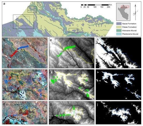
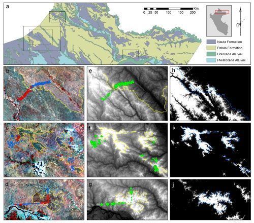
2.1. Study Areas

We gathered remotely-sensed and field data for three study areas in northwestern Amazonia (Figure 1(a)): the interfluvial zone between the Pastaza and Tigre rivers (here referred to as “Pastaza-Tigre”; Figure 1(b,e,g)); the interfluvial zone between the Curaray and Arabela rivers (“Curaray”; Figure 1(c,f,i)); and the interfluvial zone between the Amazon, Sucusari, and Apayacu rivers (“Sucusari”; Figure 1(d,g,j)). These study areas are separated by a maximum of 500 km of primary forest, and range in size from 2,000 (Sucusari) to 16,000 (Pastaza-Tigre) square kilometers (Figure 1(a)). All three areas consist of undisturbed broadleaf evergreen rainforest typical of Amazonian lowlands. Human habitations and roads are absent from the Curaray and Sucusari study areas, and field sites were accessed by helicopter at Curaray, and by boat and foot at Sucusari. Access to the Pastaza-Tigre sites was provided by the service road for the Lot 1AB oil pipeline which runs between the Pastaza and Tigre rivers.
In addition, our study areas included known boundaries between two widespread geological formations: the Pebas and Nauta Formations (Figure 1(a); [26]). The Pebas Formation is distributed across western and central Amazonia, and consists of poorly weathered and cation-rich clay sediments deposited under low-energy, semi-marine or lacustrine conditions during the early to middle Miocene (ca. 25–10 Ma; [27,28]). The Nauta Formation, which lies above the Pebas Formation, consists of sandy, weathered and cation-poor fluvial sediments deposited under high-energy, fluvial conditions during the Late Miocene (ca. 10–5 Ma; [27,29,30]). Because of ongoing river incision and erosion during the Plio-Holocene (ca. 5 Ma to recent), large expanses of the Nauta Formation have been removed across western Amazonia, exposing the Pebas Formation beneath [31,32]. This has resulted in a patch-matrix environment in which islands of Nauta Formation remain surrounded by a Pebas Formation matrix [26]. These geological patterns are believed to have been translated into edaphic and floristic patterns [8], and this heterogeneity provided us with the opportunity to both answer the questions posed above, and to gather more information on these potentially widespread and important patterns.

2.2. Satellite Imagery

To identify remotely-sensed patterns in our study areas and compare them with field data, we downloaded SRTM and Landsat data for our study areas from the USGS National Map Seamless Server ( http://seamless.usgs.gov) and EarthExplorer service ( http://earthexplorer.usgs.gov), respectively. For each study area we used one date of Landsat imagery: 30 August 2000 for Curaray; 11 August 1996 for Pastaza-Tigre [8]; and 1 November 1987 for Sucusari [19].
We performed a preliminary manual interpretation of the Landsat imagery based on image tone. For display and interpretation of the imagery, we used full-color images in which bands 4, 5, and 7 were set to red, green, and blue, respectively. Because of the inherently low contrast in these bands, we enhanced these images using a combination of contrast stretching and spatial convolution as suggested by Tuomisto et al. [33] and Hill and Foody [14]. This enhancement was performed in three steps: histogram equalization, low pass spatial filtering using a 5 × 5 window, and histogram equalization [8] (Supporting Information Figure 1). The first step of this process increased contrast in the image and expanded the range of values used for image display. The second step reduced graininess in the image but compressed the range of values used for image display, and thus reduced image contrast. The third step again increased the contrast in the image and thus the range of values used for image display. All image enhancement was performed in ENVI v.4.9 (Exelis Visual Information Solutions, Boulder, CO, USA).
Following image enhancement, we manually interpreted the Landsat imagery for each study area based on image tone, with the intent of identifying the primary terra-firme vegetation types at each study area. At all study areas, forests growing on the Pebas Formation were characterized by light-blue or light-red tones, and forests growing on the Nauta Formation were characterized by dark-olive or dark-blue tones. In all cases, image interpretation was conducted without reference to either field data or to existing geological and vegetation maps. We manually delineated the features identified in the Landsat data, and compared them with patterns observed for plants and soils in the field (see Section 2.3).
For our quantitative comparisons between Landsat imagery and field data, we used both raw Landsat imagery and imagery that had been processed to remove the across-path radiometric gradient reported by Toivonen et al. [25] (Supporting Information 1). This radiometric gradient is observed in all six non-thermal Landsat bands (i.e., bands 1–5, and band 7), and generally consists of a linear trend from higher, brighter values in the northwest to lower, darker values in the southeast. This gradient is known to be problematic when mosaicking neighboring images [25], but may also interfere with the interpretation of individual images. To remove this trend we generated linear trend surfaces for each band of Landsat imagery for each study area, and subtracted this trend surface from the raw imagery. We then used the detrended bands 3 and 4 for each study are to generate detrended normalized differential vegetation index (NDVI) images for use in our comparisons (Supporting Information 1).
To quantify the relationship between the remotely-sensed data, and our plant and soils data, we generated 250 m buffers for each plant inventory transect [17] and calculated the mean elevation or the mean value (digital number or detrended digital number) for each Landsat band (excluding band 6) in this area for each transect. We additionally calculated the mean NDVI value for each transect, and repeated these calculations for both raw and detrended Landsat data. For the Pastaza-Tigre and Curaray study areas, these buffer areas were 1km long and 500 m wide with rounded ends, and contained an average of 550 pixels of Landsat data and 55 pixels of SRTM data. For the Sucusari study area, these buffer areas were 1 km long and 500 m wide with square ends, and contained an average of 545 pixels of Landsat data and 55 pixels of SRTM data. All calculations of mean values were performed with ArcGIS v. 10 (ESRI Inc., Redlands, CA, USA).
We additionally quantified the relationship at Pastaza-Tigre between our plant and soils data, and the combination of bands typically used for image display and manual image interpretation: bands 4, 5, and 7 [8,17]. To do this we calculated the first principal component of an image composed of bands 4, 5, and 7 using correlation matrices; and then calculated the mean value for this component within the 250 m buffers described above. For reference, we repeated this analysis using an image composed of all six non-thermal bands (i.e., bands 1–5, and band 7); and an image composed of bands 4, 5, and 7 that was enhanced for display and interpretation using the methods described above (Supporting Information 1). These analyses were repeated with both raw and detrended data, and were performed in ENVI v.4.9 (Exelis Visual Information Solutions, Boulder, CO, USA).

2.3. Field Data

To test the relationship between the remotely-sensed patterns and field data, we conducted plant species inventories and collected soil samples at a total of 160 sites in northern Peru: 65 sites at Pastaza-Tigre, 52 at Curaray, and 43 at Sucusari. Each plant inventory was accompanied by soil sampling, with the exception of sites at the Sucusari study area, where we collected soil samples for 15 of the 43 plant inventories.
Our plant inventories at Pastaza-Tigre and Curaray consisted of species lists compiled along 5 m by 500 m linear transects [8]. To generate the dense but extensive datasets needed to sample across geological formations but also detect abrupt boundaries, we limited our plant inventories to pteridophytes (ferns and lycophytes). These plants are known to represent the majority of the floristic pattern observed in tree inventories, but are easier to inventory and thus require much smaller time investment [3436]. For our inventories, we only included individuals with at least one leaf (for ferns) or stem (for lycophytes) longer than 10 cm, and epiphytic and climbing individuals were recorded only if they had green leaves ≤2 m above ground. We deposited vouchers for all species in herbaria in Peru (AMAZ and USM) and Finland (TUR) (herbarium acronyms according to Index Herbariorum [37]). At Sucusari, our plant inventories consisted of species lists along 1 km segments of a continuous 2 m × 43 km linear transect [19]. Otherwise our plant inventories at Sucusari were identical to those at Pastaza-Tigre and Curaray.
At Pastaza-Tigre and Curaray we collected soil samples at 50 m, 250 m, and 450 m along each transect [8]. Each of these three samples consisted of five subsamples of the top 10 cm of mineral soil, collected in an area of 4 m × 4 m and combined in the field into a single sample. For analysis, we combined equal dry weights of the three samples per transect into a single sample, and these were analyzed at MTT Agrifood (Jokioinen, Finland) for pH; loss on ignition (a measure of organic matter content); P concentration (Bray method); and the concentration of extractable Al, Ca, K, Mg and Na (in 1 M ammonium acetate). In addition, percentages of sand, silt and clay were determined at MTT Agrifood (Curaray samples; sieving and pipette methods) and at the University of Turku Department of Geology (Turku, Finland; Pastaza-Tigre samples; laser diffraction). At Sucusari, we collected soil samples at fifteen positions along the 43 km transect, and these were assigned to the 1 km segment in which they were located. These soil samples consisted of five subsamples of the top 5 cm of mineral soil, collected in an area of 5 m × 5 m and pooled in the field. These samples were analyzed at MTT Agrifood for the same texture and chemistry variables described above for Pastaza-Tigre and Curaray.

2.4. Data Analysis

We used hierarchical agglomerative cluster analysis to identify the dominant floristic patterns in each of our three study areas [8,38]. This analysis uses pairwise floristic dissimilarities between sites to sequentially group sites into progressively larger groups, beginning with the most similar sites. For this analysis we quantified pairwise compositional dissimilarities between sites using the one-complement of the Jaccard similarity index, and classified all sites into two groups using the unweighted pair-group method with arithmetic averages (UPGMA). All calculations were performed with PC-ORD v. 4.41 (MjM Software, Gleneden Beach, OR, USA). These groups were then used to visualize the compositional patterns in the study area and to model them based on elevation data (described below).
We additionally used nonmetric multidimensional scaling (NMDS) to reduce the main floristic gradient at each study area to a single variable for comparison to Landsat data and elevation. We calculated one-dimensional NMDS solutions for our plant inventories for each study area, using the one-complement of the Jaccard index as a distance measure; a maximum of 400 iterations from 40 random starting configurations; and an instability criterion of 105. All NMDS calculations were performed with PC-ORD v. 4.41.
We used simple regression analyses to calculate the relationship between elevation or Landsat data, as independent variables; and floristic or soil gradients as dependent variables. For these analyses, the floristic gradient at each study area was represented by a single NMDS axis; the soil gradient was represented by the log-transformed sum of the concentration of four cations (Ca, Mg, Na, and K); elevation was represented by the mean elevation per transect, as calculated from the SRTM data; and Landsat data were represented by the mean band value (digital number or detrended digital number) or NDVI value, as calculated from the Landsat data. For our comparisons of Landsat data with floristic or soils data, we excluded transects which contained clouds in the Landsat data (3 of 43 transects at Sucusari). In all cases we report the coefficient of determination (r2) for the linear regressions.
To assess the ability of SRTM digital elevation data to model floristic patterns in Amazonian forests, we used classification and regression tree (CART) analysis to identify, for each study area, the elevation that best divided the plant transects into the two groups identified by the clustering analysis [39]. We then used this value to threshold the SRTM elevation data, and visually compared the classified SRTM image to the manual interpretations of the study areas generated from Landsat data. All CART analyses were performed with JMP v. 8 (SAS Institute, Cary, NC, USA)

3. Results

3.1. Image Interpretation

Manual interpretations of Landsat imagery for our three study areas identified two dominant vegetation types (Figure 1(b–d)): areas of dark-olive or dark-blue tones in Landsat imagery corresponding to higher elevations in SRTM data; and areas of light-blue or light-red tones in Landsat imagery corresponding to lower elevations. The boundaries between these features corresponded closely to the boundaries between the Nauta and Pebas Formations, respectively, as indicated by national geological maps (Figure 1(a)). In addition, the relative elevations of the features corresponded to those expected for these two formations, i.e., the Nauta Formation consistently lay above the Pebas Formation. We manually delineated these features and sampled them for plants and soils in the field.

3.2. Floristic and Edaphic Patterns

The boundaries identified in the Landsat and SRTM data corresponded to abrupt changes in plant species composition. At all three study areas, the two groups of sites identified by our cluster analysis corresponded almost perfectly to the remotely-sensed and geological boundaries (Figure 1(b–d)). The average turnover in plant species between the Pebas Formation and Nauta Formation groups was 86% at Pastaza-Tigre, and 77% at both Curaray and Sucusari (one-complement of the Jaccard index, expressed as a percentage). In total, our plant inventories included 147, 127, and 129 species at Pastaza-Tigre, Curaray, and Sucusari, respectively, with a mean of 34, 30, and 32 species per transect.
These boundaries also corresponded to abrupt changes in soil cation availability (Figure 1(e–g)). On average, the transition from the Nauta Formation to the Pebas Formation was associated with a 7-fold increase in soil cation concentrations at Curaray and Sucusari, and a 10-fold increase at Pastaza-Tigre (sum of concentrations of Ca, Mg, Na, and K). Overall, soil cation concentrations at our three study areas ranged from 0.17 to 22.58 cmol(+)·kg−1 at Pastaza-Tigre, 0.37 to 21.26 cmol(+)·kg−1 at Curaray, and 0.29 to 9.31 cmol(+)·kg−1 at Sucusari, similar to the ranges reported previously by Higgins et al. [8].
To compare the patterns in our floristic data with those in the remotely-sensed data, we used NMDS to compress the main floristic gradient at each study area into a single dimension. These single-axis ordinations captured 90%, 80%, and 86% of the variation in floristic dissimilarities in the original datasets at the Pastaza-Tigre, Curaray, and Sucusari areas, respectively, indicating strong compositional patterns in these data. These compositional gradients, furthermore, were strongly correlated with edaphic gradients. Variation along the soil cation gradient explained 90%, 71%, and 84% of the variation along the floristic gradient at Pastaza-Tigre, Curaray, and Sucusari, respectively (measured as the coefficient of determination, r2, between NMDS scores and the log-transformed sum of four cations: Ca, Mg, Na, and K).

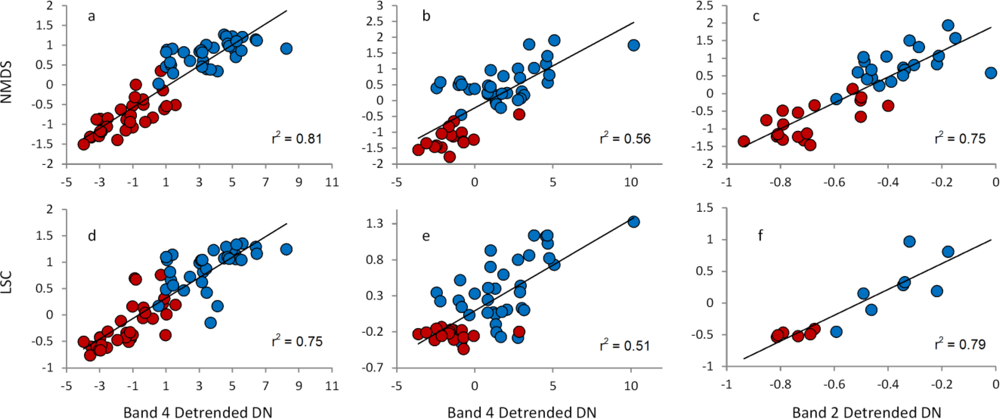
3.3. Relationships between Field Data and Landsat Data

The strong relationship observed between the Landsat imagery and field data was supported by our regression analyses. In all study areas we were able to predict the majority of the variation along floristic and edaphic gradients using one or more Landsat bands (Tables 1 and 2). At both Pastaza-Tigre and Curaray, band 4 and NDVI were consistently strongly associated with floristic composition, and predicted 68% and 75% of variation along the floristic gradient, respectively, at Pastaza-Tigre, and 55% and 53% at Curaray (Table 1). Band 4 and NDVI were also strongly associated with soil properties at these areas, and predicted 68% and 75% of variation along the soil cation gradient at Pastaza-Tigre, and 54% and 43% at Curaray (Table 2). These relationships differed at Sucusari, where bands 2 and 7 best predicted variation along the floristic gradient (coefficients of determination of 56% and 64%, respectively), consistent with previous findings [19]; and bands 2 and 1 best predicted variation along the soil cation gradient (coefficients of determination of 74% and 56%, respectively).
Detrending the Landsat data often improved these relationships substantially. This was particularly true at Pastaza-Tigre, which is the largest study area and thus most strongly affected by the across-path radiometric gradient (Supporting Information 1). Using detrended imagery, NDVI and band 4 predicted 83% and 81%, respectively, of the variation along the floristic gradient at Pastaza-Tigre, and 78% and 75% of the variation along the soil cation gradient (Tables 1 and 2). These improvements between floristic and Landsat data were much smaller at Curaray and Sucusari, and we did not observe any improvement at these study areas in relationships between Landsat data and soil data. In summary, the best individual bands for predicting plant species composition and soil properties were the detrended band 4 at Pastaza-Tigre and Cuaray, and the detrended band 2 at Sucusari. Scatterplots of these relationships demonstrate the strength of this relationship, and the clear differences in Landsat and field data between sites on the Nauta Formation and sites on the Pebas Formations (Figure 2).
We next tested the relationship between the imagery used for our manual image interpretations (Figure 1(b–d)) and our field data. The first principal component of an image for Pastaza-Tigre composed of bands 4, 5, and 7 predicted 61% and 75% of variation along the floristic gradient using raw and detrended Landsat data, respectively, and 60% and 68% of variation along the edaphic gradient (Table 3). These relationships were similar or weaker when this analysis was repeated with all six non-thermal bands (i.e., bands 1–5, and band 7), indicating that no information about floristic patterns is lost by excluding bands 1 to 3 from image display and manual image interpretation. Moreover, the methods used here to enhance the Landsat images for display and manual interpretation worsened their relationship with the floristic and soils data by 10% to 20% (Table 3).

3.4. Modeling of Floristic Patterns Based on SRTM Data

The clear relationship observed between our SRTM digital elevation data and floristic data (Figure 1(e–g)) was supported by our regression analyses. Variation in elevation explained 33%, 35%, and 73% of variation along the floristic gradient at Pastaza-Tigre, Curaray, and Sucusari, respectively (P < 0.001). On the basis of this relationship, and on the broader hypothesis that geology, as reflected in geomorphology, controls floristic composition, we used CART analysis to identify the elevation at each study area that best divided the transects into the two groups recognized by the cluster analysis in Figure 1(b–d)). We then thresholded the SRTM data using these elevations (243 m at Pastaza-Tigre, 252 m at Curaray, and 144 m at Sucusari), resulting in predicted maps of the two dominant vegetation types for the two study areas (Figure 2(h–j)). In all cases, these maps revealed zones or islands of Nauta Formation forests standing above and surrounded by a matrix of Pebas Formation forests. The match between these maps, and the manual interpretations and field data in Figure 1, was almost perfect, demonstrating the utility of SRTM data for identifying geological and floristic patterns in this region.
Despite the strong relationship between elevation and the floristic gradients at our three study areas, elevation was a relatively poor predictor of soil properties, and explained 21% (P < 0.001), 11% (P < 0.007), and 56% (P < 0.002) of variation along the soil cation gradients at Pastaza-Tigre, Curaray, and Sucusari, respectively. We believe the relationship between geomorphology and soil properties may be confounded by local and regional factors (see Section 4), and that these correlations may thus underestimate the true relationship between these variables.

4. Discussion

Using a network of 160 plant inventories distributed across 500 km of Amazonian forest, we found that Landsat imagery predicts up to 83% of the variation in plant species composition in these forests. We further found that Landsat imagery predicts up to 78% of the variation in soil cation concentrations, due probably to the strong relationship between plant species composition and soil properties. In addition, we found that variations in elevation (SRTM data) predict up to 73% of the variation in plant species composition in these forests, and that simple thresholding of SRTM data can be used to map local patterns in plant species composition. These findings provide further evidence of the great utility of Landsat imagery and SRTM digital elevation data for identifying floristic and edaphic patterns in Amazonian forests [1421]. We contend that Landsat and SRTM data, in combination with rapid taxa-based field inventory, should serve as the basis for survey and conservation planning in these vast and remote forests.
Our findings are strongly consistent with results from other locations in Amazonia [1421], but differ in four respects. First, we found that the radiometric gradient observed by Toivonen et al. [25] substantially weakens the relationship between Landsat data and plant species composition; that removing this gradient can greatly improve this relationship; and that this effect is greater over larger distances. Second, we found that the methods typically used for manual interpretation of imagery, such as contrast stretching or image smoothing, do not improve the numerical relationship between field and Landsat data, and may actually weaken this relationship. Third, despite consistently strong relationships between Landsat and field data, we find substantial differences between sites in the strength of this relationship for individual bands. At our Sucusari study area, bands 2 and 7 are most strongly correlated with both soil properties and plant species composition, consistent with findings at sites in Ecuador and northeastern Peru [15,17]. However, at our two sites in northern Peru (Pastaza-Tigre and Curaray), band 4 is most strongly correlated with these variables and band 2 is weakly or not correlated. The reasons for these differences are not clear, but may be due to atmospheric conditions, seasonality, or differences in the vegetation itself. In all of these cases, however, bands 4, 5, and 7 are significantly correlated with soil properties and floristic composition, and we believe that these bands are the most useful for image interpretation. Last, this study is one of the first to demonstrate a relationship between SRTM elevation data and floristic composition [15], and particularly to use SRTM data to predict patterns in plant species composition. Taken together, these findings demonstrate the benefits of using both elevation and Landsat data for mapping floristic or edaphic patterns in these forests.
These findings raise two questions about the use of Landsat and SRTM data for identifying floristic and edaphic patterns in these forests. First, what is the cause of the relationship between plant species composition and Landsat TM or ETM+ bands, particularly considering that the plant groups used here are not visible in Landsat imagery? As demonstrated by previous studies, patterns in pteridophyte species composition are strongly correlated with patterns in tree species composition, including tall canopy tree species [34,35]. Thus, though the floristic patterns we observe in pteridophyte species composition are not visible in Landsat data, the corresponding patterns in canopy species composition are visible. These patterns in canopy tree composition are then translated into patterns in Landsat data by variations in leaf area, structure, or chemistry. Specifically, we suggest that tree species associated with richer soils produce greater leaf mass, thinner leaf epidermis, and smaller amounts of epidermal defensive compounds than species associated with poorer soils [40,41], resulting in higher reflectance in infrared wavelengths from mesophyll tissue. In agreement with this model, and with earlier studies [17,20], we found a positive relationship between soil cation concentrations and near-infrared reflectance, meaning that richer-soil forests are brighter in Landsat imagery, and poorer-soil forests darker (Figure 1(b–d); Tables 1 and 2).
Second, what is the cause of the relationship between elevation and floristic composition? Plant species composition is known to change along elevation gradients due to changes in air temperature, precipitation, and soil moisture [42]. It is, however, unlikely that variations in these factors are responsible for the patterns observed in our study areas, as the average difference in elevation between sites in our two floristic groups is only 33, 37, and 22 m at Pastaza-Tigre, Curaray, and Sucusari, respectively. Instead, the modest changes in elevation observed here are indicators of the transition between two geological formations with profoundly different histories and edaphic characteristics: the overlying, young, and relatively cation-poor Nauta Formation; and the underlying, ancient, and relatively cation-rich Pebas Formation [43]. This interpretation is confirmed by our soil data and national geological maps (Figure 1(a,e–g); [26]), and supports the use of SRTM data to identify geological patterns, and by extension floristic patterns.
Indeed, simple classification of SRTM data for our three study areas produces predicted maps of floristic classes that match remarkably well with both our field data and geological maps (Figure 1). It must be noted, however, that the changes in elevation observed here are small in comparison to the broader trend in elevation across western Amazonia, from lower elevations in the east to higher elevations in the west, introduced by the Andean uplift. The average elevation at our Pastaza-Tigre and Curaray study areas is 100 m higher than at our Sucusari study area, substantially greater than the average difference in elevation of approximately 20 m between the Nauta and Pebas Formations [8]. As such, modeling floristic composition on the basis of elevation data is useful over limited areas, but we do not recommend the use of simple SRTM thresholding for broader regional analyses.
Despite the consistent relationship between elevation and floristic composition, elevation was a relatively poor predictor of soil properties. Two factors might confuse this relationship. First, differences in elevation as measured by the SRTM data reflect not only local variations due to transitions between geological formations, but also broad-scale regional trends due to the Andean orogeny, from northwest to southeast. These broader trends may mask the effects of local geomorphology, and we would expect this effect to be particularly strong in our largest and westernmost study area (Pastaza-Tigre). In addition, cation-rich soils at lower elevations (i.e., in the Pebas Formation) may be contaminated by poorer sediments from higher elevations (e.g. the Nauta Formations), as these poorer sediments are transported downhill by erosion and slumping. We expect this to be particularly true in patchy environments such as our Curaray study area. Despite these confounding factors, the relationships between elevation (i.e., geology), soils, and floristic composition at our study areas are sufficiently robust that elevation patterns are translated into clear floristic patterns.
This study has three possible limitations. First, all three of our study areas contained steep environmental and compositional gradients, and this likely contributed to the strong relationships observed between our remotely-sensed and field data. It is thus likely that this relationship may be weaker over narrower environmental gradients. This said, previous research at a site with a substantially narrower soil gradient [17] has found similar results to those reported here, suggesting that these methods may apply to a range of edaphic and compositional gradients. Moreover, the study areas described here are relatively homogenous compared to other sites in western Amazonia [20]. These facts argue for the general applicability of our methods. Second, this and previous studies of the relationship between Landsat and floristic data have largely been conducted in equatorial and relatively aseasonal environments, and have relied on single dates of Landsat imagery [1519]. As such, the strength of this relationship in seasonal forests exhibiting greater phenological change is difficult to predict. Fortunately, Landsat data has been used to identify broad forest types at a site in southern Peru [14], indicating that these methods may also apply across a broad range of phenological conditions. Last, in order to generate the large number of inventories needed to sample across these geological formations and their boundaries, we depended on rapid, taxa-based sampling in which we restricted our inventories to a single group of plants (ferns and lycophytes). This method is known to reproduce the majority of tree compositional patterns at distances ranging from 10 s to 100 s of kilometers [34,35], but taxa-based inventory cannot be guaranteed to work at larger or smaller scales than for which it was tested [44].
Last, our findings provide evidence for widespread patch-matrix organization across northern Peru, with clear implications for conservation planning. Without exception, each of the geological boundaries sampled in this study corresponds to an abrupt and profound change in both plant species composition and soil properties, consistent with previous studies [2,79,15,19,21,43]. This indicates that geological patterns drive soil patterns, which in turn drive floristic patterns. Extrapolating from geological maps for Peru, we believe that this patch-matrix organization, consisting of islands of poor-soil Nauta Formation forests standing above a rich-soil Pebas formation matrix, will extend across northern Peru and possibly beyond, as both geological formations are widespread in the region [26]. This type of organization is undocumented for western Amazonia, and has substantial implications for the study and protection of these forests, and particularly these isolated islands [8]. For example, the habitats found on top of Nauta Formation deposits are poorly represented in the Peruvian national protected area system, as revealed by comparing national geological and protected-area maps [26,45], and our findings could be used by conservation planners to identify new candidate protected areas. These compositional and edaphic patterns may also be translated into patterns in forest function, suggesting that geological maps be used to complement and improve existing interpolation-based approaches to mapping of Amazonian forest properties [8,46].
Along these lines, the methods described here provide a rapid and cost-effective set of tools for biological survey in Amazonian forests [16]. Landsat imagery and SRTM data are free, and the simple image enhancements and interpretations described here can be performed using a range of software packages. Furthermore, the plant inventory techniques used in this analysis require the recognition of only 200 to 300 plant species, well within the reach of both students and professionals. Using this technique, individual plant inventories can typically be completed within a single day, and digital and online guides are becoming available for the plant groups used here [47]. We thus recommend a three-stage survey process for mapping across lowland Amazonia: (1) the use of paired Landsat and SRTM data to identify matching patterns, indicative of floristic patterns of geological origin; (2) the use of rapid, taxa-based inventories and soil sampling to verify these patterns; and (3) the use of targeted, intensive multi-taxa inventories to confirm the importance of these patterns for other plant and animal groups. We hope that these become routine tools for at least preliminary mapping of Amazonian forests, and that they enable the design of more compelling and effective conservation strategies for this vast and fragile wilderness.

5. Conclusions

Here we found that Landsat imagery and Shuttle Radar Topography Mission (SRTM) digital elevation data can detect floristic and edaphic patterns across broad expanses of lowland Amazonian forest. Using 160 sites distributed across 500 km of forest, we found that Landsat imagery predicted up to 83% of the variation in plant species composition (as measured by single NMDS axes) and up to 78% of the variation in soil cation concentrations (as measured by the log-transformed sum of four cations). Based on this and prior studies, we believe that bands 4, 5, and 7 are most useful for image interpretation. Furthermore, variations in elevation (SRTM data) predicted up to 73% percent of the variation in plant species composition, and we used simple thresholding of SRTM data to map patterns in plant species composition. Using this combination of field and remotely-sensed data, we were able to identify widespread patch-matrix patterns across northwestern Amazonia, with substantial implications for conservation planning and study. Our findings demonstrate that Landsat and SRTM data can provide a cost-effective means for mapping edaphic and floristic patterns in lowland Amazonian forests. We thus recommend that maps generated from a combination of remotely-sensed and field data be used as the basis for conservation prioritization and planning in these vast and remote forests.

Supporting Information 1. Landsat Image Detrending

remotesensing-04-02401-s001.pdf

Acknowledgments

For field assistance we thank Fernando Ruiz (Pastaza-Tigre study area); Sulema Castro, Glenda Cardenas, and Wilber Bosmediano (Curaray study area); and Abel Sarmiento and Melchor Aguilar (Sucusari study area). For soil analyses, we thank Tapio Salo (MTT Agrifood Research Center, Finland) and Irma Puttonen. For logistic support at the Pastaza-Tigre study area we thank colleagues at the Instituto de Investigaciones de la Amazonia Peruana and the Universidad Nacional de la Amazonia Peruana. Additional logistic support at Pastaza-Tigre was provided by the PlusPetrol corporation (Argentina); logistic support at Curaray was provided by Repsol Exploracion Peru (Peru) and Global Geophysical Services (USA); and logistic support at Sucusari was provided by Explorama Tours (USA, Peru), and in particular Peter Jenson. We thank three anonymous reviewers for their constructive comments on the manuscript. This publication is contribution #9 of the Smithsonian Institution’s Conservation Education and Sustainability Peru Biodiversity Program. Funding for this work was provided by the John D. and Catherine T. MacArthur Foundation (USA), the Grantham Foundation for the Protection of the Environment (USA), the Carnegie Institution for Science (USA), the National Science Foundation (USA), the Academy of Finland (Finland), the American–Scandinavian Foundation (USA), Duke University (USA), and Repsol Exploracion Peru (Peru). We thank the Instituto Nacional de Recursos Naturales (Peru) for permission to collect plant specimens; the ACEER Foundation (Peru, USA) for permission to work at the Sucusari study area; and the communities of the Rio Tigre for permission to work in their forests.

References

  1. Margules, C.R.; Pressey, R.L. Systematic conservation planning. Nature 2000, 405, 243–253. [Google Scholar]
  2. Duivenvoorden, J.F.; Lips, J.M. Ecología del paisaje del Medio Caquetá: Mapas; Estudios en la Amazonia Colombiana III B; Tropenbos: Bogotá, Colombia, 1993; Volume 3. [Google Scholar]
  3. Condit, R.; Pitman, N.; Leigh, E.G.; Chave, J.; Terborgh, J.; Foster, R.B.; Nunez, P.; Aguilar, S.; Valencia, R.; Villa, G.; Muller-Landau, H.C.; Losos, E.; Hubbell, S.P. Beta-diversity in tropical forest trees. Science 2002, 295, 666–669. [Google Scholar]
  4. Malhi, Y.; Baker, T.R.; Phillips, O.L.; Almeida, S.; Alvarez, E.; Arroyo, L.; Chave, J.; Czimczik, C.I.; Di Fiore, A.; Higuchi, N.; et al. The above-ground coarse wood productivity of 104 Neotropical forest plots. Glob. Change Biol 2004, 10, 563–591. [Google Scholar]
  5. Pitman, N.C.A.; Terborgh, J.W.; Silman, M.R.; Nunez, P.; Neill, D.A.; Ceron, C.E.; Palacios, W.A.; Aulestia, M. Dominance and distribution of tree species in upper Amazonian terra firme forests. Ecology 2001, 82, 2101–2117. [Google Scholar]
  6. ter Steege, H.; Pitman, N.C.A.; Phillips, O.L.; Chave, J.; Sabatier, D.; Duque, A.; Molino, J.F.; Prevost, M.F.; Spichiger, R.; Castellanos, H.; von Hildebrand, P.; Vasquez, R. Continental-scale patterns of canopy tree composition and function across Amazonia. Nature 2006, 443, 444–447. [Google Scholar]
  7. Duivenvoorden, J.F. Tree species composition and rain forest-environment relationships in the Middle Caqueta Area, Colombia, NW Amazonia. Vegetatio 1995, 120, 91–113. [Google Scholar]
  8. Higgins, M.A.; Ruokolainen, K.; Tuomisto, H.; Llerena, N.; Cardenas, G.; Phillips, O.L.; Vasquez, R.; Rasanen, M. Geological control of floristic composition in Amazonian forests. J. Biogeogr 2011, 38, 2136–2149. [Google Scholar]
  9. Phillips, O.L.; Vargas, P.N.; Monteagudo, A.L.; Cruz, A.P.; Zans, M.E.C.; Sanchez, W.G.; Yli-Halla, M.; Rose, S. Habitat association among Amazonian tree species: A landscape-scale approach. J. Ecol 2003, 91, 757–775. [Google Scholar]
  10. Pitman, N.C.A.; Mogollon, H.; Davila, N.; Rios, M.; Garcia-Villacorta, R.; Guevara, J.; Baker, T.R.; Monteagudo, A.; Phillips, O.L.; Vasquez-Martinez, R.; et al. Tree community change across 700 km of lowland Amazonian forest from the Andean foothills to Brazil. Biotropica 2008, 40, 525–535. [Google Scholar]
  11. Tuomisto, H.; Ruokolainen, K.; Yli-Halla, M. Dispersal, environment, and floristic variation of western Amazonian forests. Science 2003, 299, 241–244. [Google Scholar]
  12. Rodriguez, E.; Morris, C.S.; Belz, J.E. A global assessment of the SRTM performance. Photogramm. Eng. Remote Sensing 2006, 72, 249–260. [Google Scholar]
  13. Tucker, C.J.; Grant, D.M.; Dykstra, J.D. NASA’s global orthorectified Landsat data set. Photogramm. Eng. Remote Sensing 2004, 70, 313–322. [Google Scholar]
  14. Hill, R.A.; Foody, G.M. Separability of tropical rain-forest types in the Tambopata-Candamo Reserved Zone, Peru. Int. J. Remote Sens 1994, 15, 2687–2693. [Google Scholar]
  15. Salovaara, K.J.; Thessler, S.; Malik, R.N.; Tuomisto, H. Classification of Amazonian primary rain forest vegetation using Landsat ETM plus satellite imagery. Remote Sens. Environ 2005, 97, 39–51. [Google Scholar]
  16. Thessler, S.; Ruokolainen, K.; Tuomisto, H.; Tomppo, E. Mapping gradual landscape-scale floristic changes in Amazonian primary rain forests by combining ordination and remote sensing. Glob. Ecol. Biogeogr 2005, 14, 315–325. [Google Scholar]
  17. Tuomisto, H.; Poulsen, A.D.; Ruokolainen, K.; Moran, R.C.; Quintana, C.; Celi, J.; Canas, G. Linking floristic patterns with soil heterogeneity and satellite imagery in Ecuadorian Amazonia. Ecol. Appl 2003, 13, 352–371. [Google Scholar]
  18. Tuomisto, H.; Ruokolainen, K. Variación de los Bosques Naturales en las Áreas Piloto a lo Largo de Transectos y en Imágenes de Satélite. In Evaluación de Recursos Forestales no Maderables en la Amazonía Noroccidental; Duivenvoorden, J.F., Balslev, H., Cavelier, J., Grández, C., Tuomisto, H., Valencia, R., Eds.; IBED, Universiteit van Amsterdam: Amsterdam, The Netherlands, 2001; pp. 63–96. [Google Scholar]
  19. Tuomisto, H.; Ruokolainen, K.; Aguilar, M.; Sarmiento, A. Floristic patterns along a 43-km long transect in an Amazonian rain forest. J. Ecol 2003, 91, 743–756. [Google Scholar]
  20. Tuomisto, H.; Ruokolainen, K.; Kalliola, R.; Linna, A.; Danjoy, W.; Rodriguez, Z. Dissecting Amazonian biodiversity. Science 1995, 269, 63–66. [Google Scholar]
  21. Ruokolainen, K.; Tuomisto, H. Vegetación natural de la zona de Iquitos. In Geoecología y Desarrollo Amazonico: Estudio Integrado en la zona de Iquitos, Perú; Kalliola, R., Flores, S., Eds.; Annales Universitatis Turkuensis Ser A II: Turku, Finland, 1998; Volume 114, pp. 253–365. [Google Scholar]
  22. Rossetti, D.F.; Valeriano, M.M. Evolution of the lowest Amazon Basin modeled from the integration of geological and SRTM topographic data. Catena 2007, 70, 253–265. [Google Scholar]
  23. Asner, G.P.; Knapp, D.E.; Broadbent, E.N.; Oliveira, P.J.C.; Keller, M.; Silva, J.N. Selective logging in the Brazilian Amazon. Science 2005, 310, 480–482. [Google Scholar]
  24. Oliveira, P.J.C.; Asner, G.P.; Knapp, D.E.; Almeyda, A.; Galvan-Gildemeister, R.; Keene, S.; Raybin, R.F.; Smith, R.C. Land-use allocation protects the Peruvian Amazon. Science 2007, 317, 1233–1236. [Google Scholar]
  25. Toivonen, T.; Kalliola, R.; Ruokolainen, K.; Malik, R.N. Across-path DN gradient in Landsat TM imagery of Amazonian forests: A challenge for image interpretation and mosaicking. Remote Sens. Environ 2006, 100, 550–562. [Google Scholar]
  26. INGEMMET, Mapa Geológico del Perú; Instituto Geologico Minero Y Metalurgico: Lima, 2000.
  27. Hoorn, C.; Wesselingh, F.P.; ter Steege, H.; Bermudez, M.A.; Mora, A.; Sevink, J.; Sanmartin, I.; Sanchez-Meseguer, A.; Anderson, C.L.; Figueiredo, J.P.; et al. Amazonia through time: Andean uplift, climate change, landscape evolution, and biodiversity. Science 2010, 330, 927–931. [Google Scholar]
  28. Räsänen, M.E.; Linna, A.M.; Santos, J.C.R.; Negri, F.R. Late miocene tidal deposits in the Amazonian Foreland Basin. Science 1995, 269, 386–390. [Google Scholar]
  29. Rebata, L.A.; Gingras, M.K.; Räsänen, M.E.; Barberi, M. Tidal-channel deposits on a delta plain from the Upper Miocene Nauta Formation, Marañon Foreland Sub-basin, Peru. Sedimentology 2006, 53, 971–1013. [Google Scholar]
  30. Figueiredo, J.; Hoorn, C.; van der Ven, P.; Soares, E. Late Miocene onset of the Amazon River and the Amazon deep-sea fan: Evidence from the Foz do Amazonas Basin. Geology 2009, 37, 619–622. [Google Scholar]
  31. Räsänen, M.E.; Salo, J.S.; Jungner, H.; Pittman, L.R. Evolution of the western Amazonian lowland relief: Impact of Andean foreland dynamics. Terra Nova 1990, 2, 320–332. [Google Scholar]
  32. Roddaz, M.; Baby, P.; Brusset, S.; Hermoza, W.; Darrozes, J.M. Forebulge dynamics and environmental control in Western Amazonia: The case study of the Arch of Iquitos (Peru). Tectonophysics 2005, 399, 87–108. [Google Scholar]
  33. Tuomisto, H.; Linna, A.; Kalliola, R. Use of digitally processed satellite images in studies of tropical rain-forest vegetation. Int. J. Remote Sens 1994, 15, 1595–1610. [Google Scholar]
  34. Ruokolainen, K.; Linna, A.; Tuomisto, H. Use of Melastomataceae and pteridophytes for revealing phytogeographical patterns in Amazonian rain forests. J. Trop. Ecol 1997, 13, 243–256. [Google Scholar]
  35. Ruokolainen, K.; Tuomisto, H.; Macia, M.J.; Higgins, M.A.; Yli-Halla, M. Are floristic and edaphic patterns in Amazonian rain forests congruent for trees, pteridophytes and Melastomataceae? J. Trop. Ecol 2007, 23, 13–25. [Google Scholar]
  36. Jones, M.M.; Tuomisto, H.; Olivas, P.C. Differences in the degree of environmental control on large and small tropical plants: Just a sampling effect? J. Ecol 2008, 96, 367–377. [Google Scholar]
  37. Thiers, B. Index Herbariorum: A Global Directory of Public Herbaria and Associated Staff. New York Botanical Garden’s Virtual Herbarium. Available online: http://sweetgum.nybg.org/ih/ (accessed on 20 June 2012).
  38. Legendre, P.; Legendre, L. Numerical Ecology; Elsevier: Amsterdam, The Netherlands, 1998; Volume 20, pp. 1–853. [Google Scholar]
  39. Breiman, L.; Friedman, J.H.; Olshen, R.A.; Stone, C.J. Classification and Regression Trees; Wadsworth and Brooks/Cole: Monterey, CA, USA, 1984. [Google Scholar]
  40. Fine, P.V.A.; Mesones, I.; Coley, P.D. Herbivores promote habitat specialization by trees in Amazonian forests. Science 2004, 305, 663–665. [Google Scholar]
  41. Asner, G.P.; Martin, R.E. Canopy phylogenetic, chemical and spectral assembly in a lowland Amazonian forest. New Phytol 2011, 189, 999–1012. [Google Scholar]
  42. Lieberman, D.; Lieberman, M.; Peralta, R.; Hartshorn, G.S. Tropical forest structure and composition on a large-scale altitudinal gradient in Costa Rica. J. Ecol 1996, 84, 137–152. [Google Scholar]
  43. Vormisto, J.; Tuomisto, H.; Oksanen, J. Palm distribution patterns in Amazonian rainforests: What is the role of topographic variation? J. Veg. Sci 2004, 15, 485–494. [Google Scholar]
  44. Higgins, M.; Ruokolainen, K. Rapid tropical forest inventory: A comparison of techniques based on inventory data from western Amazonia. Conserv. Biol 2004, 18, 799–811. [Google Scholar]
  45. UNEP-WCMC. World Database on Protected Areas (WDPA) Annual Release 2009. Available online: http://www.wdpa.org/AnnualRelease.aspx (accessed on 20 June 2009).
  46. Anderson, L.O. Biome-scale forest properties in Amazonia based on field and satellite observations. Remote Sens 2012, 4, 1245–1271. [Google Scholar]
  47. Zuquim, G.; Costa, F.R.C.; Prado, J.; Tuomisto, H. Guide to the Ferns and Lycophytes of REBIO Uatumã, Central Amazonia; Instituto Nacional de Pesquisas da Amazônia: Manaus, Brazil, 2008. [Google Scholar]
Figure 1. Geological, edaphic, and floristic patterns at three study areas in northern Peru. (a) Geological map for Peru [26], overlaid with the extents of the three study areas: from left to right, Pastaza-Tigre, Curaray, and Sucusari. Solid lines indicate extents of panels (bj), with exception of panel (h), whose extent is indicated by broken lines. Inset shows location of (a) relative to map of Peru. (b–d) Plant inventories, divided into two groups by clustering analysis (red and blue points), and superimposed upon enhanced and detrended Landsat images for the Pastaza-Tigre, Curaray, and Sucusari study areas, respectively. (e–g) Soil cation concentrations superimposed upon Shuttle Radar Topography Mission (SRTM) digital elevation data, where the diameter of the circles is proportional to the sum of the concentrations of four cations (Ca, Mg, Na, and K). Lighter tones in the SRTM data indicate higher elevations; order of panels is as in (b–d). (h–j) Results of simple classification of SRTM data, where white pixels are above the elevation threshold and black pixels are below the elevation threshold; order as in (b–d). Yellow lines in (b–g) and blue lines in (h–j) indicate manual interpretations of Landsat imagery.
Remotesensing 04 02401f1
Figure 2. Scatterplots for selected regressions in Tables 1 and 2. Plots depict the relationship between either detrended band 4 or detrended band 2 of Landsat data (measured by detrended digital numbers, ‘DN’), and either the main floristic gradient (measured by a single nonmetric multidimensional scaling axis; ‘NMDS’) or the soil cation gradient (measured as the log-transformed sum of the concentrations of Ca, Mg, Na, K; ‘LSC’), for three study areas in northern Peru. Points represent individual sites, and are colored according to clustering memberships in Figure 1. (a) and (d) Pastaza-Tigre study area. (b) and (e) Curaray study area. (c) and (f) Sucusari study area. (a–c) Correspond to results from Table 1. (d–f) Correspond to results from Table 2. R2 values for each regression are indicated in the bottom-right of each panel.
Remotesensing 04 02401f2
Table 1. Relationship between Landsat and floristic data for three study areas in northern Peruvian Amazonia. Values are the coefficients of determination (r2) for linear regressions between individual Landsat bands (measured by digital numbers or detrended digital numbers) or NDVI as independent variables, and the main floristic gradient (measured by a single NMDS axis) as dependent variables, based on either unprocessed (“Raw”) or detrended (“Detrended”) Landsat images. All values are significant at P < 0.001, with the exception of values in parentheses. The two highest r2 values for each image are presented in bold.
Pastaza-TigreCuraraySucusari
BandRawDetrendedRawDetrendedRawDetrended
10.32(0.11)(0.01)(0.01)0.270.24
2(0.07)0.40(0.04)(0.06)0.560.75
30.400.23(0.10)(0.11)(0.17)(0.11)
40.680.810.550.560.340.24
50.400.55(0.03)0.200.550.39
70.470.58(0.00)(0.12)0.640.50
NDVI0.750.830.530.51(0.20)(0.11)
Table 2. Relationship between Landsat and soils data for three study areas in northern Peruvian Amazonia. Values are the coefficient of determination (r2) for linear regressions between individual Landsat bands (measured by digital numbers or detrended digital numbers) or NDVI as independent variables, and the soil cation gradient (as measured by the log-transformed sum of the concentrations of Mg, Ca, Na, and K) as dependent variables, based on either unprocessed (“Raw”) or detrended (“Detrended”) Landsat images. All values are significant at P < 0.001, with the exception of values in parentheses. The two highest r2 values for either each image are presented in bold.
Pastaza-TigreCuraraySucusari
BandRawDetrendedRawDetrendedRawDetrended
10.19(0.07)(0.00)(0.00)(0.56)(0.37)
2(0.09)0.31(0.06)(0.06)0.740.79
30.380.26(0.04)(0.06)(0.38)(0.26)
40.680.750.540.51(0.22)(0.08)
50.390.49(0.03)(0.12)(0.23)(0.08)
70.420.49(0.01)(0.08)(0.35)(0.19)
NDVI0.750.780.430.42(0.08)(0.01)
Table 3. Relationship between Landsat data, and either floristic or soils data, for Pastaza-Tigre sites. Values are the coefficient of determination (r2) for linear regressions between the floristic gradient (measured by a single NMDS axis) or the soil cation gradient (measured by the log-transformed sum of the concentrations of Ca, Mg, Na, and K) as independent variables, and the first principal component of the indicated bands as dependent variables, for either unprocessed (“Raw”) or detrended (“Detrended”) imagery. “Enhanced” indicates use of the contrast adjustments and spatial convolution indicated in Section 2.3. All r2 values are significant at P < 0.001.
Independent VariableImageryAll BandsBands 4, 5, 7Bands 4, 5, 7, Enhanced
Floristic compositionRaw0.520.610.53
Detrended0.750.750.65

SoilsRaw0.530.600.50
Detrended0.690.680.58

