Article

Comparative Analysis of Four Models to Estimate Chlorophyll-a Concentration in Case-2 Waters Using MODerate Resolution Imaging Spectroradiometer (MODIS) Imagery

1
Centre Eau Terre Environnement, INRS, 490 de la Couronne, Québec, QC G1K 9A9, Canada
2
Département de Mathématiques et de Statistique, Université de Moncton, 18 avenue Antonine-Maillet, Moncton, NB E1A 3E9, Canada
*
Author to whom correspondence should be addressed.
Remote Sens. 2012, 4(8), 2373-2400; https://doi.org/10.3390/rs4082373
Submission received: 12 June 2012 / Revised: 27 July 2012 / Accepted: 2 August 2012 / Published: 13 August 2012

Abstract

:
The occurrence and extent of intense harmful algal blooms (HABs) have increased in inland waters during recent decades. Standard monitor networks, based on infrequent sampling from a few fixed observation stations, are not providing enough information on the extent and intensity of the blooms. Remote sensing has great potential to provide the spatial and temporal coverage needed. Several sensors have been designed to study water properties (AVHRR, SeaBAM, and SeaWIFS), but most lack adequate spatial resolution for monitoring algal blooms in small and medium-sized lakes. Over the last decade, satellite data with 250-m spatial resolution have become available with MODIS. In the present study, three models inspired by published approaches (Kahru, Gitelson, and Floating Algae Index (FAI)) and a new approach named APPEL (APProach by ELimination) were adapted to the specific conditions of southern Quebec and used to estimate chlorophyll-a concentration (Chl-a) using MODIS data. Calibration and validation were provided from in situ Chl-a measured in four lakes over 9 years (2000–2008) and concurrent MODIS imagery. MODIS bands 3 to 7, originally at 500-m spatial resolution, were downscaled to 250 m. The APPEL, FAI, and Kahru models yielded satisfactory results and enabled estimation of Chl-a for heavy blooming conditions (Chl-a > 50 mg·m−3), with coefficients of determination reaching 0.95, 0.94, and 0.93, respectively. The model inspired from Gitelson did not provide good estimations compared to the others (R2 = 0.77). However, the performance of all models decreased when Chl-a was below 50 mg·m−3.

1. Introduction

Sustainable management of water resources became a real interest for the international community a few decades ago. Although Canada holds 9% of the renewable supply of freshwater for 0.5% of the worldwide population [1], this precious resource needs to be managed responsibly. Evidence that a lot of countries currently suffer from water penury cannot be denied [2]. Globally, the origin of the penury is attributed in part to the deterioration of water quality caused by the development of Harmful Algal Blooms (HABs), such as cyanobacterial blooms. The increasing development of such HABs reflects the advanced state of aquatic ecosystem eutrophication caused by urban, agricultural, and industrial developments. Once established in lakes, cyanobacterial populations are extremely difficult to control except through the long-term reduction of nutrient inputs from the watershed and from internal sources.
Currently, the most common way to detect the presence of blooms is in situ sampling, generally through riverine claims [3]. However, neither the spatial distribution nor the temporal frequency of such monitoring programs is sufficient to detect the spatial extent, intensity, and duration of HABs in water bodies, especially during periods of heavy blooms [4], and for a country like Canada that covers a very large area with a great number of lakes. In situ sampling and sample analyses are laborious, and the results obtained are often difficult to interpret because of HAB heterogeneous spatial distribution and sudden rise and fall [5]. In addition, standard in situ sampling and sample analyses are expensive. More than $650,000 CAN was spent to collect and analyze in situ samples from 150 water bodies in the province of Quebec alone during 2009 [6].
Remote sensing, with its synoptic viewing, consistent recurrence and capacity to provide information over a wide range of wavelengths represents an attractive alternative method to monitor algal blooms. Satellite sensors that provide data in visible and near infrared (NIR) wavelengths can be used to estimate chlorophyll-a concentration (Chl-a) based on its high absorption of the blue and red part of the electromagnetic spectrum, and its high reflectance of the green and NIR wavebands. Thus, bio-optical models that relate the apparent optical properties of water bodies to their inherent optical properties can be used to estimate Chl-a [7].
To date, however, the use of satellite data has been limited to open ocean waters classified as Case-1 waters, in which phytoplankton and co-varying material of biological origin are the principal constituents responsible for variations in ocean inherent optical properties [8] and algal pigments are often the only component optically active in the water [9]. Remote sensing data have been efficiently used to detect marine algal blooms in recent decades [1014]. The basic approach has been to model the apparent optical properties of oceans from remote sensing data as a function of Chl-a alone [15]. However, while the estimation of Chl-a is a relatively easy task for Case-1 water, monitoring algal blooms in lakes and coastal water classified as Case-2 waters is a challenging one. The remote sensing reflectance (R) spectra of these water bodies is generally complex because of the presence of many optically active components, such as chlorophylls and carotenoids from phytoplankton and aquatic plants, total suspended solids (TSS), colored dissolved organic matter (CDOM), and sometimes bottom reflectance [16]. Generally, the algorithms developed to detect blooms based on the absorption properties of a single variable absorbing near 700 nm (typical of Chl-a) are inadequate for this type of waters [15]. Furthermore, the older generation of sensors dedicated to the study of water properties lack sufficient spatial resolution to assess Chl-a in Case-2 waters. Nevertheless, recently, sensors such as the MODerate Resolution Imaging Spectroradiometer (MODIS) and the MEdium Resolution Imaging Spectrometer (MERIS), with their full spatial resolution of 250 m and 300 m respectively, are increasingly used to achieve this goal. This makes the two sensors very concurrent in such applications. Also, many other sensors were used successfully, such as Landsat TM to retrieve Chl-a and suspended solid concentrations in lake Kasumigaura using neural network technique [9] and to develop an algorithm for assessing phycocyanin concentrations in lake Erie in order to improve the understanding of temporal and spatial dynamics of cyanobacterial blooms. SeaWiFS data were also used to establish the seasonal distribution pattern and intensity of phytoplankton and terrigenous input [17], and AHVRR to point out the behavior of main taxonomic groups of Baikal lake phytoplankton in relation to ice conditions [18], or to assess other water quality parameters [19,20]. Recently, QuickBird and MERIS data were also used to assess cyanobacterial blooms based on their specific pigment (phycocyanin) in Lake Champlain [21]. Thus, many semi-analytical algorithms [12,2226] and indexes [13] are now available in the literature to retrieve the Chl-a concentration of inland water bodies.
For this study, because of the large number of days with cloud cover over the selected lakes and the relatively low number of in situ measurements, we chose to use MODIS (revisit time of 1 day) rather than MERIS (revisit time of 3 days) in order to collect enough data for model calibration and validation. The first two of the 36 MODIS bands in the red/NIR have 250-m spatial resolution. The rest of the visible and infrared (IR) bands which are the most appropriate for the detection of Chl-a, CDOM and suspended particles have resolutions larger than 250-m. However, the spatial resolution of MODIS bands 3 to 7 can be downscaled from 500- to 250-m spatial resolution using the approach of Trishchenko et al. [27]. In this manner, the first seven bands of MODIS sensor become available at 250-m spatial resolution, covering the visible, NIR, and IR parts of the spectrum. It is important to notice that the bands originally at 250-m spatial resolution and those downscaled were originally designed for aerosol, cloud and land applications. The MODIS bands designed for surface water studies are at 1-km spatial resolution, which is not optimal for monitoring algal bloom in lakes, especially in small and medium-sized ones. Thus, the challenge is to demonstrate that the first seven bands of the MODIS sensor can be used to estimate Chl-a in water bodies after spatial resolution enhancement.
The purpose of this research is to evaluate the performance of the three bio-optical models most commonly used in the literature (Kahru, Gitelson, and FAI (Floating Algae Index)) and of a novel approach named APPEL (APProach by ELimination) to estimate Chl-a in a series of lakes in the southern part of Quebec province. The assumption that MODIS bands, not originally developed for water applications, can be used to detect algal blooms in small and medium-sized inland water bodies was also tested.

2. Material and Methods
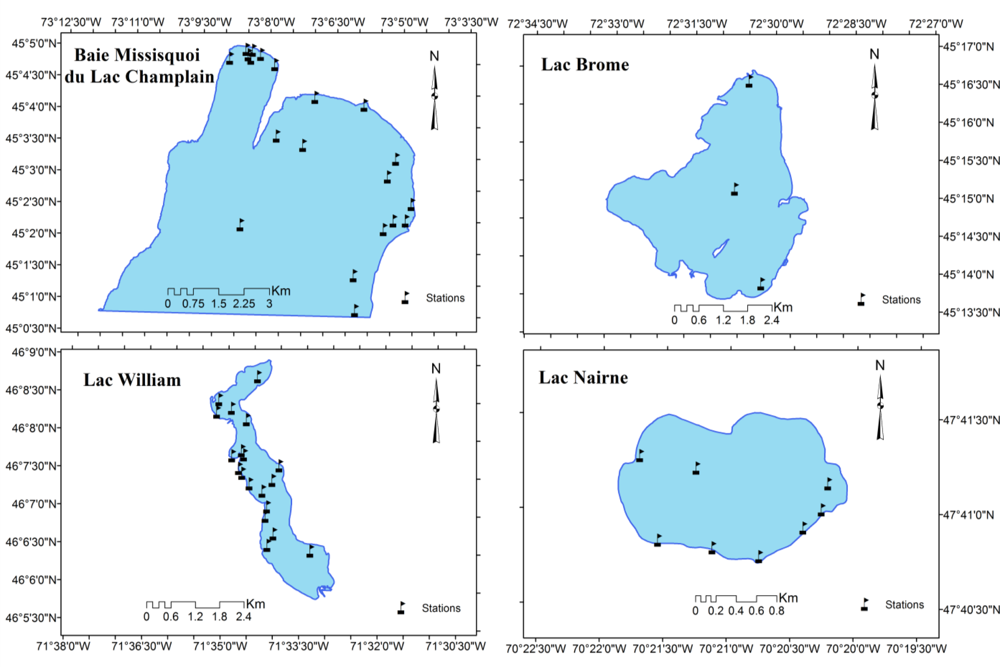
2.1. In situ Data

Four lakes were considered in this study: Missisquoi Bay of Lake Champlain, Lake Brome, Lake William, and Lake Nairne, with surfaces of 45, 41, 4, and 2 km2, respectively (Figure 1). These lakes are part of a program to monitor water bodies with recurrent cyanobacterial blooms carried out by the Ministère du Développement Durable de l’Environnement et des Parcs (MDDEP). The data were collected over a period of 9 years (2000 to 2008) at several sites on the four lakes (Figure 2) and included cyanotoxins (equivalent total microcystin-LR and anatoxin-a), algal pigments (Chl-a, pheophytine-a), phytoplankton abundance, and physicochemical characteristics of lake water (total phosphorous, total nitrogen, pH, turbidity, Secchi depth, surface temperature).
Chl-a was used as a proxy of the total algal biomass and potential indicator of HABs. A total of 168 Chl-a in situ measurements and a corresponding 62 MODIS images were obtained. Of these, 51 values were used for the model calibration/validation, corresponding to a sub-group of 22 images. The rest of the data set was unexploited due to the presence of clouds and/or cloud shadows on the measurement sites or to the bad quality of the images. The largest sample size was in Missisquoi Bay (N = 37) and the smallest was in Lake Brome (N = 6). The concentration of Chl-a varied between 2.5 mg·m−3 (Lake Nairne, 2007) and 91,000 mg·m−3 (Missisquoi Bay of Champlain Lake, 2003).
A second data set collected by the MDDEP over 5 years (2004 to 2008) was used for field truth validation. These data contained two kinds of observations: (1) field maps where the spatial distribution of algal blooms is delimited, and (2) records of observations made by technicians from regional directorates of the MDDEP as to whether blooms were present on a lake or not. It is important to note that no laboratory analysis was made for this data set. We used this latter to evaluate the ability of the models to detect the presence of algal blooms by comparing in situ observations to the corresponding dates of MODIS images.

2.2. MODIS Data

The remote sensing data used were acquired by the MODIS sensor aboard the TERRA platform of NASA’s Earth Observation System (EOS). The MODIS Level 1B product is a set of geo-located and calibrated data. The MODIS sensor operates across a very wide spectrum, with 36 bands that cover the region from 0.4 to 14.4 μm, observing with a spatial resolution varying from 250 m to 1 km. Sensor data are available from the website ( http://ladsweb.nascom.nasa.gov/data/search.html) in HDF format. The satellite passes over the study site between 2:00 and 4:30 pm GMT on an ascending orbit. For this study, images from 2000 to 2008 were downloaded and pre-processed. Only the first seven MODIS bands were utilized, the first two being available at 250 m spatial resolution, and bands 3 to 7 available at 500 m but downscaled to 250 m. Table 1 summarizes the characteristics of the bands used in this study.
Two pre-processing steps were performed: spatial resolution downscaling and atmospheric correction. Downscaling entails three phases. Phase 1: Downscaling of the MODIS/Terra bands 3–7 at 250 m spatial resolution using adaptive regression and radiometric normalization, as described in Trishchenko et al. [27]. Phase 2: Improvement of the spatial resolution by re-projecting the images from the Sinusoidal to the Lambert conformal conic (LCC) projection. Originally, the L1B products of MODIS data are projected on a sinusoidal system, introducing a substantial distortion of areas distant from the central meridian. However, the LCC superimposes a cone over the Earth sphere with two reference parallels secant to the globe and intersecting it, which minimizes distortion when projecting a three-dimensional surface to a two-dimensional surface, and enhances the quality of the spatial resolution especially in North-American and polar zones. Phase 3: Production of clear sky, cloud, and cloud shadow masks by applying a scene identification algorithm. The algorithm uses an exclusive criteria sequence. Bare grounds are identified and excluded, based on a high contrast of reflectance between the band-1 and band-6. Thereafter, snow and ice pixels are excluded, followed by water pixels and cloud pixels. After excluding all classes above, the remaining pixels likely belong to cloud free land class.
Recent works clearly show that atmospheric correction found to be significant in water applications, especially in NIR part of the spectrum [2830]. Several atmospheric correction models are available and can be divided into two categories: deterministic such as MODTRAN [31], EXACT [32], 6S [33] or SMAC [34], and empirical like empirical line method [35] and the dark pixel or histogram method [36]. However, it has been shown that the most effective atmospheric correction algorithms are the simplest [30]. Thereby in our work, the MODIS data were corrected using the SMAC model (Simplified Method for Atmospheric Correction), a simplified and operational version of the 5S codes (Simulation of the Satellite Signal in the Solar Spectrum), because it can perform an atmospheric correction within a short time [34]. All pre-processing steps (downscaling, re-projection, production of a clear-sky mask and atmospheric correction) were performed using an automatic tool developed by the Canadian Centre for Remote Sensing [37].

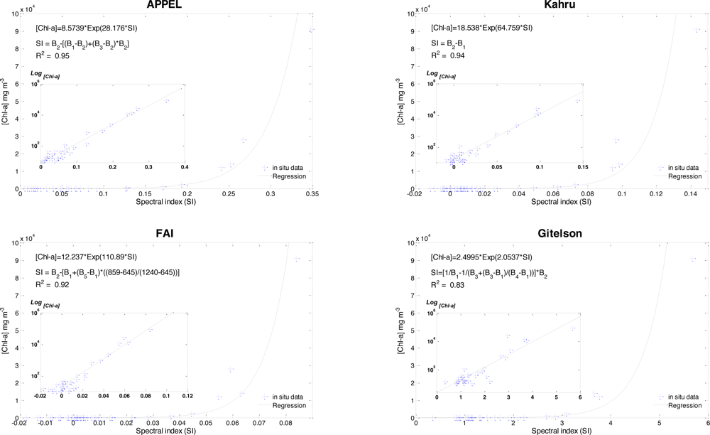
3. Algorithms Used to Estimated Chl-a Concentration
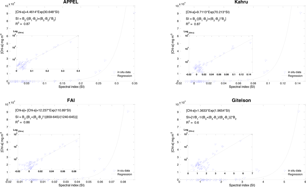
Three semi-empirical algorithms (Kahru, Gitelson, and FAI (Floating Algae Index)) and a novel approach named APPEL (APProach by ELimination) developed at the remote sensing laboratory of the Institut National de la Recherche Scientifique (INRS), Quebec, were selected for this study. Many Case-2 water models designed to estimate Chl-a using remote sensing data are already in use [11,38,39], but most rely on the typical signal of Chl-a near 700 nm, which is not covered by the first seven bands of the MODIS sensor (Table 1). The MODIS bands originally designed for ocean color studies, which do cover 700 nm, are at 1-km spatial resolution, which is not suitable for small and medium-sized water bodies. The purpose of the present study is to assess the potential of the first seven MODIS bands to estimate Chl-a at 250-m spatial resolution. These bands do not cover the frequency of maximal Chl-a absorption, but their better spatial resolution might compensate for their lack of spectral resolution. This assumption is supported by several studies [4042]. Although originally designed for land studies and cloud detection, by comparison to sensors such as Landsat-7 ETM+, CZCS (Coastal Zone Color Scanner) and SeaWiFS, the MODIS 250 m and 500 m bands have potential for water applications as they are 4–5 times more sensitive than L7/ETM+ bands, nearly twice as sensitive as the corresponding CZCS blue-green bands, and 3–4 times more sensitive than the red and NIR ones, while they are only 1–2 times (500 m, blue-green) less sensitive than the corresponding SeaWiFS bands [19].

3.1. Kahru’s Model

Most Chl-a estimation models have been based on the ultraviolet (UV) and the visible part of the spectrum [10,4345]. This is not problematic for Case-1 waters, but there are many problems associated with the use of algorithms based on this part of the spectrum for Case-2 waters, especially in the UV portion, where several complications arise in relation to atmospheric correction [46] and the overestimation of Chl-a due to the presence of CDOM and TSS [47].
The semi-analytical approach of Kahru uses the red/NIR part of the spectrum [13]. MODIS band-1 has been shown to be sensitive to changes in concentrations of cyanobacteria grown in cultures and has therefore been suggested for the qualitative mapping of cyanobacterial blooms [48], while MODIS band-2 has been successfully used to quantify algal blooms in the Baltic Sea [49]. Kahru et al. [26] suggested using MODIS band 1, 3, and 4 as true-color images to detect the presence of blooms, and as a quantitative quantification, they proposed using the difference between band-2 and band-1 as a water surface turbidity index. Turbidity is not specific to algal blooms (e.g., suspended solids can result from erosion within the drainage basin), but when mainly caused by phytoplankton biomass, turbid features appear in blue-green in the true-color image. Thus, in this case the turbidity index can be used as an estimator of Chl-a. This approach has been successfully used to detect an algal bloom in Paracas Bay in Peru [26] and to monitor water quality in the southwestern US reservoir system [14].

3.2. Floating Algae Index (FAI)

Chuanmin and Ming-Xia developed an ocean color index to detect floating algae based on red, NIR, and shortwave infrared (SWIR) [50]. This part of the spectrum was used because water strongly absorbs these wavelengths. Thus, water appears opaque (black) even in the most turbid environments. Floating algae on the water surface, on the other hand, have higher reflectance in the NIR than other wavelengths and thus can be easily distinguished from the surrounding clear waters [13].
The FAI avoids the problems related to ocean indexes such as NDVI (normalized difference vegetation index) and EVI (enhanced vegetation index) when applied to the detection of floating algal blooms. The latter two indexes have been useful for delineating floating algae from adjacent water, but the pixel values of floating algae and adjacent waters are sensitive to variable environmental and observing conditions such as aerosols and solar/viewing geometry. These variable conditions create difficulties in visualization and quantification since they affect the visual contrast between floating algae and adjacent waters in addition to change their absolute values [13]. Thus, the FAI is defined as the difference between reflectance in the NIR (RNIR) and a corrected reflectance of this band by the red and the SWIR bands (R′NIR):
FAI = R NIR R NIR '
where
R NIR ' = R R + ( R SWIR R R ) * ( λ NIR λ R ) / ( λ SWIR λ R )
R′NIR is the baseline reflectance in the NIR band derived from linear interpolation between the red and SWIR bands. For MODIS, λR = 645 nm, λNIR = 859 nm, and λSWIR = 1,240 nm [13]. The FAI is then calculated as follows:
FAI = R ( λ b 2 ) [ R ( λ b 1 ) + ( R ( λ b 5 ) R ( λ b 1 ) ) * ( λ b 2 λ b 1 ) / ( λ b 5 λ b 1 ) ]
The FAI has been successfully used to detect an extensive bloom of a floating green macroalgae, Enteromorpha prolifera, in open ocean near Qingdao in China under a range of atmospheric environments (clear, hazy, and sunlight conditions) [50] and to reconstruct the temporal frequency and spatial distribution of cyanobacterial blooms over 9 years (2000–2008) in Taihu Lake in China [51] using MODIS data.

3.3. Gitelson Model

The principle of the Gitelson model is based on the relation between the detected reflectance and the total absorption and backscattering coefficients [52].
R rs ( λ ) γ b b ( λ ) ( a tot ( λ ) ) + b b ( λ )
where γ depends of the radiation emerging from water, bb is the backscattering coefficient, and atot (λ) is the sum of the absorption coefficients of phytoplankton cells (apigm), CDOM (aCDOM), non-algal particles or TSS (atripton), and pure water (aw) as shown in the following equation:
a tot ( λ ) = a pigm ( λ ) + a CDOM ( λ ) + a tripton ( λ ) + a w ( λ )
This semi-analytical model uses three bands to estimate Chl-a that relates pigment concentration to reflectance, R(λi) [53], defined as:
[ Chl a ] [ R 1 ( λ 1 ) R 1 ( λ 2 ) ] * R ( λ 3 )
The reflectance reciprocal of the first band, R 1 ( λ 1 ) a tot ( λ 1 ) + b b b b, must be strongly sensitive to Chl-a absorption (λ1 falls within the 660–690 nm range) [54]. However, R−1(λ1) is also affected by TSS, CDOM and pure water absorption, and backscatter from particulate matter. This effect (denominator of Equation (6)) can be minimized using a second spectral band, where R−1(λ2) is the least sensitive to Chl-a absorption and the nearest to λ1. It has been demonstrated that λ2 must belong to the 710–730 nm range [12,54]. The difference between R−1(λ1) and R−1(λ2) thus eliminates the effects of TSS and CDOM, but Equation (6) is still affected by backscattering. A third band, λ3 is therefore used to reduce the influence of bb. This band must be the least affected by pigments, TSS and CDOM, and the total absorption is a measure of pure water. The NIR range corresponds to this condition (a(λ3)∼aw) [55,56]. The output of these bands combination is mostly dependent on Chl-a. Thus, the model takes the following form:
[ R 1 ( λ 1 ) R 1 ( λ 2 ) ] * R ( λ 3 ) a chla ( λ 1 )
The two-band combination R−1(λ1) * R−1(λ3) ∝ achla(λ1) is a special case of this conceptual model, where apigm(λ1) ≫ bb and apigm(λ1) ≫ atripton(λ1) + aCDOM(λ1) [22]. To test the performance of this approach, the Gitelson model was used to estimate Chl-a of Chesapeake estuary [12].
However, the λ1 and λ2 wavelengths used in this approach do not fall within the coverage of the first seven MODIS bands. Since λ1 must strongly respond to Chl-a, it should belong to the blue or red parts of the spectrum. Due to the aforementioned problems when using the blue region of the spectrum, we chose MODIS band-1 as the band of maximum Chl-a absorption. Regarding λ2, used to minimize the effect of TSS and CDOM, Wei et al. [57] demonstrated that MODIS band-3 could explain up to 88% of the variance in turbidity of Poyang Lake in China [57] (turbidity being an index of TSS). In addition, Hu et al. [19] found that bands 1, 3, and 4 have the potential to detect CDOM in turbid water, as they were able to explain between 59 and 80% of the variance of CDOM concentration. In the present study we use a combination of MODIS bands 1, 3, and 4 as a substitute for the wavelength of λ2 used in Gitelson’s model:
λ 2 ( substuted ) ( R b 3 + Δ R b 3 Δ R b 4 )
where
Δ R b 3 = R b 3 R b 1
Δ R b 4 = R b 4 R b 1
In this equation, Rb3 is used to minimize the effect of TSS, and the ratio ( Δ R b 3 Δ R b 4 ) is used to minimize the effect of CDOM. The third band, λ3 should fall in the NIR according to Gitelson. MODIS band-2 was chosen for this purpose. Therefore, the final new formulation of the model inspired from the Gitelson approach was as follows:
[ Chl a ] [ R 1 ( λ b 1 ) R 1 ( λ b 3 + λ Δ b 3 λ Δ b 4 ) ] * R ( λ b 2 )

3.4. Novel Approach APPEL (APProach by ELimination)

The principle of APPEL is similar to that of the Gitelson approach. All of the MODIS bands capture signals responding to Chl-a, CDOM, TSS, and particle backscattering (bb) from water bodies, but they do so in varying proportions according to the wavelength range of each band. The maximum reflectance of phytoplankton cells is in the NIR, where water has its minimum reflectance (Figure 3). Therefore, the maximum information regarding Chl-a can be derived from MODIS band-2. However, this band is affected by CDOM, TSS, and particle backscattering, as expressed by the following relation:
R ( λ b 2 ) α [ Chl a ] + [ CDOM ] + [ TSS ] + b b
To minimize the effect of CDOM, we have to use a band that is highly sensitive to the presence of organic matter and captures a maximum of reflection. Luciani et al. [58] have shown that organic matter has maximal reflection in the region of 400–470 nm [58]. This range corresponds to MODIS band-3. However, since band-3 is also affected by Chl-a and bb, a second band that is highly sensitive to the presence of Chl-a is also required. MODIS band-2 achieves this purpose, as the maximum reflectance of Chl-a is in the NIR. The same band is also used to reduce the effect of bb from the water, since water strongly absorbs in the NIR; Gitelson et al. [54] also used this region to minimize the effect of bb [55,56].
To minimize the effect of TSS, we proceed the same way as above. For this purpose, a third band is used, where the maximum of reflectance captured by the band is due to the presence of TSS. Hu et al. [19] have demonstrated that MODIS band-1 is highly correlated to the presence of TSS [19]. As above, we use MODIS band-2 to minimize the effect of Chl-a on MODIS band-1; no minimization of particle backscattering is needed because MODIS band-1 is in the red part of the spectrum, where water absorbs strongly. Thereby, particle backscattering is already feeble.
Equation (12) is then a function of Chl-a only, and the APPEL Model can be written as follows:
APPEL = R ( λ b 2 ) [ ( R ( λ b 3 ) R ( λ b 2 ) ) * R ( λ b 2 ) + ( R ( λ b 1 ) R ( λ b 2 ) ) ]

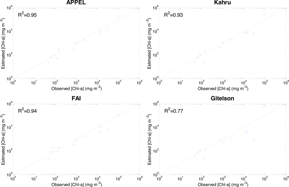
4. Accuracy Assessment

Four indexes are used to evaluate the performance of the models: coefficient of determination (R2), relative bias (BIASr), relative root mean square error (RMSEr), and relative Nash–Sutcliffe efficiency (Nr). The latter evaluates model performance by comparing the accuracy of estimated values to the observed mean value of the entire data set. If the result is negative, the estimate is worse than using the mean value; the criterion is equal to one for a perfect estimation. We chose to use the relative form of the indexes in order to reduce the contrast between the observed and estimated high values and the lower ones. Because the absolute forms of the indexes quantify absolute differences, over- or under-estimates of high values have, in general, greater influence than those of lower values. By using the relative forms of the indexes, we reduce, for example, the influence of the absolute differences recorded during periods of heavy blooms. Similarly, the influence of the absolute differences recorded during periods of no blooming are enhanced [59]. The equations of the indexes are as follows:
R 2 = [ i = 1 n ( O i O ¯ ) ( Es Es ¯ ) i = 1 n ( O i O ¯ ) 2 i = 1 n ( Es i Es ¯ ) 2 ] 2
BIASr = 1 n i = 1 n ( Es i O i Es i )
RMSEr = 1 n i = 1 n ( Es i O i ) Es i ) 2
Nr = 1 i = 1 n ( O i Es i O i ) 2 i = 1 n ( O i O ¯ O ¯ ) 2
where n is the sample size, O and Es are the observed and estimated values, and Ō and Es ¯ are the means of the observed and estimated values.

5. Results and Discussion

5.1. Evaluation of Downscaling the MODIS Band Signal

MODIS bands 3 to 7, originally at 500-m spatial resolution, were downscaled to 250-m. To ensure that the downscaling process did not affect the signal of the original bands, we compared the spectral index of the downscaled images to that of the originals.
Figure 4 shows the correlation between the MODIS signal sampled from areas on lakes captured on three images from three different years (2001–2003). The y-axis corresponds to the spectral index of the downscaled image, and the x-axis to the spectral index of the original image (500-m spatial resolution) re-sampled to 250 m using a method that does not enhance the resolution of the image but simply divides the surface of each pixel into four (from 500 × 500 m to 250 × 250 m).
The results show a significant correlation between the original and downscaled signals (R2 varies from 0.94 to 0.98). However, for a proper model assessment, the gradient “a” (the slope of the regression equation Y=a*X+b) should be used as a weighting index:
wr 2 = { | a | * r 2 for a 1 , | a | 1 * r 2 for a > 1
In this manner, under- or overestimations are also taken into account [59]. According to Equation (18), the weighted correlation coefficients are respectively 0.88, 0.77, and 0.82 for bands 3, 4, and 5. This means that the downscaled images lose from 12 to 23% of their original signal quality, which is acceptable since the MODIS band signal is 4 to 5 times higher than the corresponding bands of other sensors such as Land-Sat7/ETM or CZCS [19].

5.2. Model Calibration

As depicted in Figure 5, all models show a good correlation between Chl-a and the spectral index derived from MODIS data by each model, except for the Gitelson-inspired model, which does not perform as well. However, the models produce only a small error at high Chl-a values, with most of the error coming from low concentrations.
The World Health Organization (WHO) has established an alert threshold for water utilization of 10 mg·Chl-a·m−3 [60]. Water bodies with Chl-a lower than this threshold are not considered dangerous for recreational activities. Thus, to minimize a potential error related to high in situ data dispersion at low Chl-a, samples with in situ concentrations below 10 mg·m−3 were removed from the data set to test the accuracy of each model. As anticipated, the accuracy of the recalibrated models was improved (Figure 6). Therefore, most of the error was produced from low Chl-a values. This is not surprising, since most of the studied models (APPEL, Kahru, and FAI) are based on the red/NIR part of the spectrum where water has very low reflection. This means that water appears transparent when biomass is low, and the reflected signal is very weak (Figure 4), which increases the noise/signal ratio of the bands precluding a good correlation between Chl-a and the spectral index. Also, at low Chl-a the algal community is more likely to be composed of a larger diversity of species [61], generating a larger diversity of optical signatures obtained by the satellite. Other considerations may also help to explain the high dispersion observed at low Chl-a. (1) The MODIS sensor bands cover a relatively broad range of the electromagnetic spectrum, possibly lowering their sensitivity at low Chl-a. (2) The atmospheric correction (SMAC) can produce additional noise; this would be especially apparent at low Chl-a. (3) The downscaling procedure may have caused a loss of signal quality. An additional source of noise can also be associated to in situ sampling of Chl-a, as positioning the sampling sites on the satellite images was difficult. The MDDEP technicians did not have GPS to locate their positions, and thus the sampling locations recorded were approximate. To overcome this problem, we averaged the satellite spectral index from four pixels around each in situ sampling site during the calibration step.

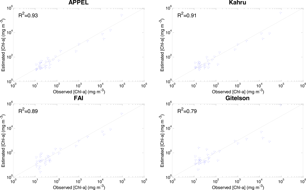
5.3. Model Validation

To evaluate the accuracy of the four models studied, a cross-validation technique was applied. This technique involves temporarily removing a given value of Chl-a from the sampling data set and using the remaining observations as a calibration group to estimate the withdrawn value. This operation is repeated for the whole data set. The performance of each model was assessed using the performance indexes presented above.
All models except Gitelson-inspired model produced satisfactory results (Table 2). The Nash criterion values of the APPEL, Kahru, and FAI models were quite similar and indicated very good correspondence between observed and estimated Chl-a (i.e., close to 1), with the APPEL and Kahru models performing slightly better than the FAI. The Nash criterion value of the Gitelson-inspired model was much lower (Nr = 0.34). RMSEr results showed that the Chl-a estimates calculated with the APPEL model were more precise than those of the other models (RMSEr of APPEL < Kahru < FAI < Gitelson). However, the error in Chl-a estimates was relatively high for all models, since the best performance produced a RMSEr of 69%. Moreover, relative BIAS results were negative for all of the models, indicating that all tended to underestimate Chl-a. Again, the APPEL model showed the best performance (–17%), while the other models ranged from −23% to −87%.
The poor performance of the Gitelson-inspired model can be explained by the inability of the available MODIS bands to optimally respond to Chl-a absorption. The Chl-a pigment has two large absorption peaks (absorption maxima around 430 and 680 nm), with an optimized range of absorption between 660 and 690 nm. The MODIS band-1 used in the Gitelson-inspired model is indeed sensitive to a region where this pigment absorbs, but it is not centered on its maximal absorption. In addition, λ2, used to minimize the effect of TSS and CDOM, utilizes bands 1, 3, and 4 in this model, which are also sensitive to the presence of Chl-a. Consequently, the λ1 wavelength shift and the λ2 band substitution may be the cause of the lower performance of this model. APPEL, Kahru, and FAI, on the other hand, are based on the contrast between the water and Chl-a reflectance in the red/NIR part of the spectrum. In this spectral region, pixels of Chl-a are easily distinguished from water pixels. Thus, for this study, the models based on reflectance (APPEL, Kahru, and FAI) to estimate Chl-a were more accurate than the Gitelson-inspired model based on absorption. Figure 7 shows the Chl-a estimated by the four models as a function of the observed Chl-a. This figure shows the decrease in the dispersion of estimated values as Chl-a increases, except for the Gitelson-inspired model, where the dispersion is large for most estimated concentrations.
WHO has fixed a second threshold (Chl-a > 50 mg·m−3), with stricter recommendations than the earlier-mentioned threshold for recreational water use (10 mg·m−3), at which water utilization should be avoided (Figure 8). The performance of the models was specifically assessed for values at or above these concentrations. Thereby, the cross-validation results were divided into two groups: the first contains Chl-a between 10 and 50 mg·m−3 (N = 24), and the second contains the remaining values (above 50 mg·m−3; N = 12). The resulting evaluation indexes can be used to determine the behavior of the models in both heavy and low–moderate blooming conditions.
Tables 3 and 4 summarize the performance of the models at Chl-a values above 50 mg·m−3 and between 10 and 50 mg·m−3, respectively. In general, the performance indexes calculated for the high concentrations (Chl-a > 50 mg·m−3) show better results than those calculated for the models calibrated with all Chl-a > 10 mg·m−3, except for the Nash criterion, which shows a slight decrease in the precision of models at the high concentrations. This may be due the smaller size of sample used in this step (N = 12). Figure 9 and 10 show the scatter plots of the observed and estimated (cross-validation) Chl-a values greater than 50 mg·m−3 and between 10 and 50 mg·m−3, respectively. It is clear that the correlation is much more significant in heavy bloom conditions (Figure 9). The improvement in performance is not large for APPEL, Kahru, and the Gitelson-inspired model (Table 3), but for the FAI model, performance improves a lot when using only high Chl-a. The RMSEr changes from 119% to 58%, the BIASr from −32% to 4%, the R2 from 0.89 to 0.94, and the Nr from 0.91 to 0.93. This is not surprising since the accumulated cells form scums at the surface of the water, which will improve the accuracy of this model originally developed to monitor floating algae. At these concentrations, FAI performs as well as APPEL, slightly overestimating Chl-a by 1% and 4%, respectively, while the Kahru model underestimates Chl-a by 2%. In contrast, the BIASr of the Gitelson-inspired model remains high and does not reach the performance of the other models even for heavy algal blooms.
Model performance is much poorer at intermediate concentrations of Chl-a. Table 4 and Figure 10 clearly show the absence of significant correlation between estimated and measured Chl-a for all models except APPEL (R2 = 0.30; Nr = 0.62), with a Nash criterion value close to 0.8, which can be considered to perform acceptably. These results confirm that the error of estimates is mainly caused by low Chl-a values. Water reflectance does not exceed 20% even in heavy bloom conditions. For moderate to low bloom conditions, it is even lower (less than 8%). Consequently, the signal detected in such conditions is more affected by noise. Even under these conditions however, APPEL still has the best performance and the Gitelson-inspired model the worst, while FAI loses much more of its accuracy (Nr decreases from 0.93 to 0.34) than APPEL or Kahru.

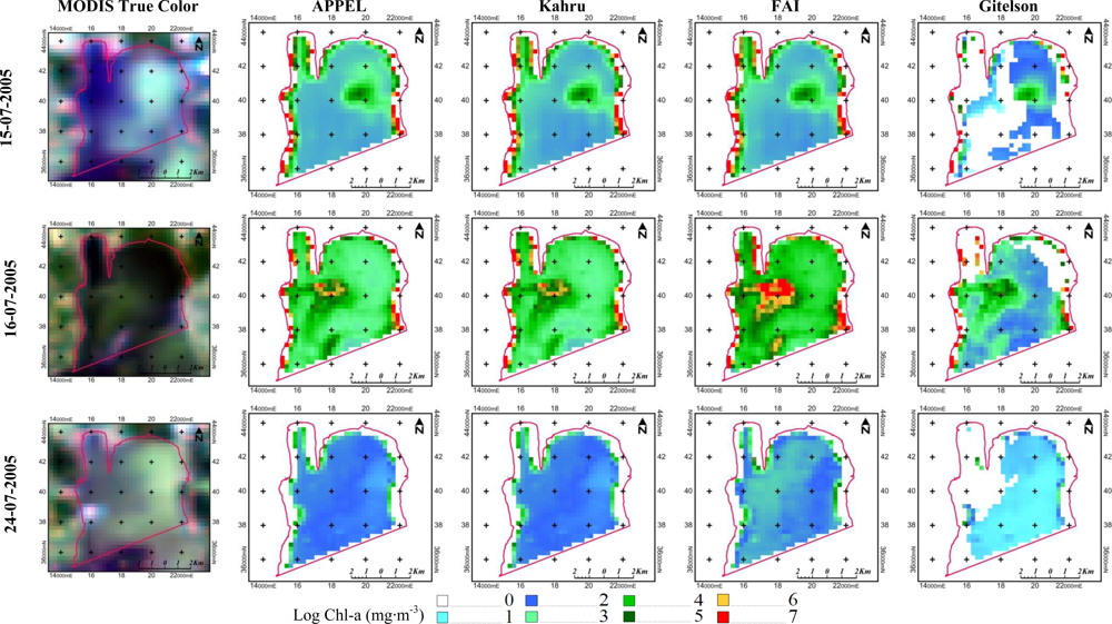
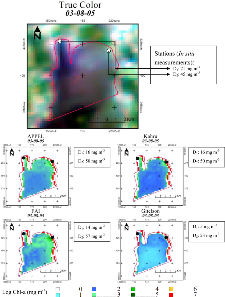
5.5. Qualitative Evaluation

Hu et al. [51] emphasized the difficulty of determining the distribution of blooms and identified three methods to evaluate its accuracy: (1) comparison of field data with concurrent high-resolution sensor observations, (2) examination of the reflectance spectra of the identified bloom, and (3) evaluation of the observed patterns against existing knowledge from historical field surveys [51]. In order to evaluate the accuracy of the four models used in the present study, we opted for the third method proposed above. The MDDEP provided historical in situ field surveys on the presence/absence of cyanobacterial blooms and a set of sketch maps showing the extent of the blooms (as described in Section 2.1). Thus, it is possible to compare the sketches drawn on field maps to the true-color images of the corresponding dates obtained from the MODIS sensor. After validating that the MODIS images revealed a bloom when the MDDEP had observed one, we applied each of the four models to the images in order to visually evaluate their ability to monitor the spatial distribution of blooms.
Figure 11 shows an example of the field map made by MDDEP technicians and the corresponding true-color image from the MODIS sensor for a bloom that took place on 19 September 2001. A clear correspondence between the sketch and the bloom extension visible on the image (green hue) can be seen both for heavy bloom conditions (the northeast to east part of the lake) and for low–moderate blooming conditions (central part of the lake). The same exercise was done for a series of bloom cases documented by the MDDEP (three dates are shown in Figure 12). In this figure, the three left-hand panels show the MODIS true-color images, and the remaining blocks of three panels show the results when the APPEL, Kahru, FAI, and Gitelson models were applied, respectively. The three consecutive dates show the progress of the algal bloom on Missisquoi Bay. The first image corresponds to the beginning of the bloom, the second depicts its expansion on the bay, and the last shows the relative extinction of the bloom episode. From Figure 11, it can be seen that all of the models detected a westward movement of the phytoplankton biomass. Since currents and swells are known to be low in bays, we conclude that the movement of this algal biomass was mainly caused by wind. In order to verify this fact, the mean wind direction of this day (15-07-2005 to 16-07-2005) was extracted from the two nearest meteorological stations (within a radius of 10 km of the bay). The average wind direction at “Sainte-Sabine” station (45°13′24.000″N; 73°01′24.000″W) was 90° (i.e., wind blowing from the east) and the average wind direction at “Frelighsburg” station (45°03′01.000″N; 72°51′42.000″W) was 140° (i.e., wind blowing from east-south-east). Therefore, the direction of the displacement of the algal bloom on the MODIS images coincides with the average wind direction at the two stations on that day. This demonstrates the capacity of remote sensing data to monitor algal blooms in inland water bodies on a daily basis.
Comparison of the bloom extension obtained from the model outputs and the true-color images (Figure 12) shows that the FAI model tends to amplify the bloom expansion, while the Gitelson-inspired model tends to reduce it compared to the results of APPEL and Kahru. The latter two models seem to better follow the spatial distribution, and this is true for all blooming conditions (low, moderate, and high). Also, in terms of bloom quantification, the APPEL and Kahru models seem to yield the same range of Chl-a, while FAI tends to give higher and Gitelson lower values compared to APPEL and Kahru. In order to spatially compare the model results to in situ measured Chl-a, Figure 13 shows two stations on Missisquoi Bay (D1 and D2) sampled by the MDDEP (data from these stations were part of the calibration data set). In this example, APPEL and Kahru are the best estimators of Chl-a, while FAI tends to overestimate the concentration in moderate bloom conditions and underestimate it under low bloom conditions, and while the Gitelson-inspired model underestimates the concentrations in all blooming conditions.
It is important to note that the largest limitation with the use of satellite-based models for operational monitoring of algal blooms is the presence of clouds that prevent the detection of the blooms and consequently their quantification. In Quebec, cloud cover (overcast) is present more than 50% of the year. However, solar radiation is known to be among the conditions that favour the development of algal blooms. Thus, blooms are more likely to occur under cloud-free conditions, a fact favoring the use of satellite data as an operational tool to monitor algal blooms and estimate their intensity. Another problem is that pixels along the edge of water bodies tend to overestimate Chl-a (see the red pixels on the shore of Champlain Lake in Figures 12 and 13). Generally, these pixels depict the combined signal from water and riparian vegetation surrounding the lakes. As most the models use the red/NIR wavelengths, most of the information detected by the sensor comes from Chl-a reflectance. Thus, the models confuse these pixels with heavy bloom conditions. In order to better distinguish water pixels from mixed (land–water) pixels, a land mask is being developed using a data set of more than 1600 MODIS images covering a period of 11 years (2000–2010).

6. Conclusions

Our aim in this study was to assess the performance of three existing models: Kahru, FAI and a model inspired from Gitelson, as well as a novel approach named APPEL for the estimation of Chl-a in southern Quebec inland waters as an indicator of water quality. One innovative element of this project is its use of the highest resolution of the first seven MODIS bands, enabling the exploitation of a wider spectral range at 250 m spatial resolution. Our results clearly demonstrate that this method can be efficiently used to monitor lake water quality as models can explain up to 95% of the variance. The analysis suggests that APPEL model yields the best overall estimates of Chl-a concentrations. However, Kahru remains a good alternative for ease of use since the model requires only the first two MODIS bands that are already at 250-m spatial resolution (no downscaling procedure needed), and it achieves performances comparable to APPEL, particularly for moderate to high Chl-a concentrations. In heavy blooming conditions, the FAI model can be considered, since it produces the lowest error under these conditions. On the other hand, all models showed poor accuracy to estimate Chl-a at low concentrations, with a slight advantage for APPEL.
The objective of this work was not to replace standard sampling methods but to provide a tool to help reducing the efforts and costs associated with in situ sampling. Firstly, the use of remotely sensed data has limitations related to the presence of clouds, and to border effects where Chl-a values can be highly overestimated. Secondly, the lower performance of all models under low Chl-a concentrations is largely explained by the low signal received from water in the NIR part of the spectrum, making the signal/noise ratio much smaller. It may also be related to the atmospheric correction process, and to the reduction in signal quality caused by the downscaling process in which up to 23% of the original signal can be lost. These factors limit the application of developed algorithms during the initiation phase of blooms corresponding to low Chl-a concentrations.
In short, the model analysis has demonstrated that (1) the first seven bands of MODIS sensor can be used to estimate Chl-a in small lakes with high accuracy during heavy bloom, and consequently this can be used as an affordable and accessible tool to manage water quality; (2) better spatial resolution can compensate for the lack of spectral resolution, since the wavebands used to estimate Chl-a yielded satisfactory results in the majority of cases albeit they are not optimal for the detection of this pigment; (3) estimating low Chl-a concentration was an issue. Since the errors related to downscaling process could not be further improved, focus should be on improvement of the atmospheric correction by testing others approaches. Dark pixel has been shown to be a promising approach and should be considered in such applications [30]; (4) none of the models was perfect, and each had its strengths and weaknesses. Development of an ‘ensemble system’ thus seems to be a favorable approach for more accurate estimates.

Acknowledgments

We thank S. Blais from the Ministère du Développement Durable, de l’Environnement et des Parcs for providing in situ data, the NASA/GSFC for making the MODIS data available, and R. Latifovic and A.P. Trishchenko from the Canadian Centre of Remote Sensing for providing the tool to downscale the resolution of MODIS bands.

References and Notes

  1. Gleick, P.H. The World’s Water; Island Press: Chicago, IL, USA, 2000; Volume 7, p. 315. [Google Scholar]
  2. Bouchard, V.M. Floraisons de Cyanobactéries au lac Saint-Augustin: Dynamique à Court Terme et Stratification; Université Laval: Québec, QC, Canada, 2004. [Google Scholar]
  3. Laurion, I.; Rousseau, A.; Chokmani, K.; Drogui, P.; Bourget, S.; Warren, A.; Drevnick, P. Mémoire sur la Situation des lacs au Québec en regard des Cyanobactéries; INRS-Centre Eau Terre Environnement: Québec, QC, Canada, 2009; p. 25. [Google Scholar]
  4. Eija, R.; Rvi, R.O.; Seija, H.L.; Juha-Markku, L.N.; Mika, R. Effect of sampling frequency on detection of natural variability in phytoplankton: Unattended high-frequency measurements on board ferries in the baltic sea. J. Marine Sci 1998, 55, 8. [Google Scholar]
  5. Agence Française de Sécurité Sanitaire des Aliments, A. Rapport sur l’Évaluation des Risques liés à la Présence de Cyanobactéries et de leurs Toxines dans les eaux Destinées à l’Alimentation, à la Baignade et autres Activités Récréatives; AFSSET: Maisons-Alfort, France, 2006; p. 231. [Google Scholar]
  6. MDDEP. Les Lacs et Cours d’Eau Touchés par une Fleur d’Eau d’Algues Bleu-Vert; MDDEP: Québec, QC, Canada, 2009; Available online: http://www.mddep.gouv.qc.ca/eau/algues-bv/bilan/saison2009/bilan2009.pdf (accessed on 12 June 2012).
  7. Carder, K.L.; Chen, F.R.; Lee, Z.P.; Hawes, S.K.; Kamykowski, D. Semianalytic moderate-resolution imaging spectrometer algorithms for chlorophyll a and absorption with bio-optical domains based on nitrate-depletion temperatures. J. Geophys. Res 1999, 104, 5403–5421. [Google Scholar]
  8. Morel, A.; Prieur, L. Analysis of variations in ocean color. Limnol. Oceanogr 1977, 22, 709–722. [Google Scholar]
  9. Baruah, P.J.; Tumura, M.; Oki, K.; Nishimura, H. Neural Network Modeling of Lake Surface Chlorophyll and Sediment Content from Landsat TM Imagery. Proceedings of 22nd Asian Conference on Remote Sensing, Singapore, 5–9 November 2001; p. 6.
  10. Ahn, Y.H.; Shanmugam, P. Detecting the red tide algal blooms from satellite ocean colour observations in optically complex Nourtheast-Asia coastal waters. Remote Sens. Environ 2006, 103, 419–437. [Google Scholar]
  11. Becker, R.H.; Sultan, M.I.; Boyer, G.L.; Twiss, M.R.; Konopko, E. Mapping cyanobacterial blooms in the great lakes using modis. J. Great Lakes Res 2009, 35, 447–453. [Google Scholar]
  12. Gitelson, A.A.; Schalles, J.F.; Hladik, C.M. Remote chlorophyll-a retrieval in turbid, productive estuaries: Chesapeake bay case study. Remote Sens. Environ 2007, 109, 464–472. [Google Scholar]
  13. Hu, C. A novel ocean color index to detect floating algae in the global oceans. Remote Sens. Environ 2009, 113, 2118–2129. [Google Scholar]
  14. Tarrant, P.; Neuer, S. Monitoring algal blooms in a southwestern U.S. Reservoir system. Eos Trans. AGU 2009, 90, 38. [Google Scholar]
  15. Darecki, M.; Stramski, D. An evaluation of modis and seawifs bio-optical algorithms in the baltic sea. Remote Sens. Environ 2004, 89, 326–350. [Google Scholar]
  16. Mishra, S.; Mishra, D.; Schluchter, W. A novel algorithm for predicting phycocyanin concentrations in cyanobacteria: A proximal hyperspectral remote sensing approach. Remote Sens 2009, 1, 758–775. [Google Scholar]
  17. Heim, B.; Oberhaensli, H.; Fietz, S.; Kaufmann, H. Variation in Lake Baikal’s phytoplankton distribution and fluvial input assessed by seawifs satellite data. Glob. Planet. Change 2005, 46, 9–27. [Google Scholar]
  18. Semovski, S.V.; Mogilev, N.Y.; Sherstyankin, P.P. Lake Baikal ice: Analysis of AVHRR imagery and simulation of under-ice phytoplankton bloom. J. Marine Syst 2000, 27, 117–130. [Google Scholar]
  19. Hu, C.; Chen, Z.; Clayton, T.D.; Swarzenski, P.; Brock, J.C.; Muller-Karger, F.E. Assessment of estuarine water-quality indicators using MODIS medium-resolution bands: Initial results from tampa bay. Remote Sens. Environ 2004, 93, 423–441. [Google Scholar]
  20. Matthews, M.W.; Bernard, S.; Winter, K. Remote sensing of cyanobacteria-dominant algal blooms and water quality parameters in Zeekoevlei, A small hypertrophic lake, using MERIS. Remote Sens. Environ 2010, 114, 2070–2087. [Google Scholar]
  21. Wheeler, S.M.; Morrissey, L.A.; Levine, S.N.; Livingston, G.P.; Vincent, W.F. Mapping cyanobacterial blooms in Lake Champlain’s missisquoi bay using Quickbird and MERIS satellite data. J. Great Lakes Res 2012, 38(Supplement 1), 68–75. [Google Scholar]
  22. Dall'Olmo, G.; Gitelson, A.A.; Rundquist, D.C.; Leavitt, B.; Barrow, T.; Holz, J.C. Assessing the potential of seawifs and modis for estimating chlorophyll concentration in turbid productive waters using red and near-infrared bands. Remote Sens. Environ 2005, 96, 176–187. [Google Scholar]
  23. Gitelson, A.A.; Dall'Olmo, G.; Moses, W.; Rundquist, D.C.; Barrow, T.; Fisher, T.R.; Gurlin, D.; Holz, J. A simple semi-analytical model for remote estimation of chlorophyll-a in turbid waters: Validation. Remote Sens. Environ 2008, 112, 3582–3593. [Google Scholar]
  24. Gitelson, A.A.; Kondratyev, K.Y. Optical models of mesotrophic and eutrophic water bodies. Int. J. Remote Sens 1991, 12, 373–385. [Google Scholar]
  25. Gons, H.J.; Rijkeboer, M.; Ruddick, K.G. A chlorophyll-retrieval algorithm for satellite imagery (medium resolution imaging spectrometer) of inland and coastal waters. J. Plankton Res 2002, 24, 947–951. [Google Scholar]
  26. Kahru, M.; Mitchell, B.G.; Diaz, A.; Miura, M. Modis detects a devastating algal bloom in Paracas Bay, Peru. EOS 2004, 85, 465–472. [Google Scholar]
  27. Trishchenko, A.P.; Luo, Y.; Khlopenkov, K.V. A method for downscaling MODIS land channels to 250 m spatial resolution using adaptive regression and normalization. Proc. SPIE 2006, 6366, 36607–36607. [Google Scholar]
  28. Kallio, K.; Attila, J.; Härmä, P.; Koponen, S.; Pulliainen, J.; Hyytiäinen, U.-M.; Pyhälahti, T. Landsat ETM+ images in the estimation of seasonal lake water quality in boreal river basins. Environ. Manag 2008, 42, 511–522. [Google Scholar]
  29. Moses, W.J.; Gitelson, A.A.; Berdnikov, S.; Povazhnyy, V. Estimation of chlorophyll-a concentration in Case II waters using modis and meris data—Successes and challenges. Environ. Res. Lett 2009, 4, 045005. [Google Scholar]
  30. Siegel, D.A.; Wang, M.; Maritorena, S.; Robinson, W. Atmospheric correction of satellite ocean color imagery: The black pixel assumption. Appl. Opt 2000, 39, 3582–3591. [Google Scholar]
  31. Ferrier, G. Evaluation of Apparent Surface Reflectance Estimation Methodologies; Taylor & Francis: Abingdon, UK, 1995; Volume 16. [Google Scholar]
  32. Popp, T. Correcting atmospheric masking to retrieve the spectral albedo of land surfaces from satellite measurements. Int. J. Remote Sens 1995, 16, 3483–3508. [Google Scholar]
  33. Vermote, E.F.; Tanre, D.; Deuze, J.L.; Herman, M.; Morcette, J.J. Second simulation of the satellite signal in the solar spectrum, 6s: An overview. IEEE Trans. Geosci. Remote Sens 1997, 35, 675–686. [Google Scholar]
  34. Proud, S.R.; Rasmussen, M.O.; Fensholt, R.; Sandholt, I.; Shisanya, C.; Mutero, W.; Mbow, C.; Anyamba, A. Improving the smac atmospheric correction code by analysis of meteosat second generation ndvi and surface reflectance data. Remote Sens. Environ 2010, 114, 1687–1698. [Google Scholar]
  35. Smith, G.M.; Milton, E.J. The use of the empirical line method to calibrate remotely sensed data to reflectance. Int. J. Remote Sens 1999, 20, 2653–2662. [Google Scholar]
  36. Chavez, P.S. Image-Based Atmospheric Corrections: Revisited and Improved; American Society for Photogrammetry and Remote Sensing: Bethesda, MD, USA, 1996; Volume 62. [Google Scholar]
  37. Trishchenko, A.P.; Luo, Y.; Khlopenkov, K.V.; Park, W.M. Multi-Spectral Clear-Sky Composites of MODIS/Terra Land Channels (B1–B7) over Canada at 250 m Spatial Resolution and 10-Day Intervals since March, 2000: Top of the Atmosphere (TOA) Data; GeoGratis Client Services: Sherbrooke, QC, Canada, 2010. [Google Scholar]
  38. Giardino, C.; Bresciani, M.; Pilkaityte, R.; Bartoli, M.; Razinkovas, A. In situ measurements and satellite remote sensing of Case 2 waters: First results from the curonian lagoon. Oceanologia 2010, 52, 197–210. [Google Scholar]
  39. González Vilas, L.; Spyrakos, E.; Torres Palenzuela, J.M. Neural network estimation of chlorophyll a from meris full resolution data for the coastal waters of galician rias (NW Spain). Remote Sens. Environ 2011, 115, 524–535. [Google Scholar]
  40. Gordon, H.R.; Wang, M. Retrieval of water-leaving radiance and aerosol optical thickness over the oceans with seawifs: A preliminary algorithm. Appl. Opt 1994, 33, 443–452. [Google Scholar]
  41. Hu, C.; Muller-Karger, F.E.; Andrefouet, S.; Carder, K.L. Atmospheric correction and cross-calibration of Landsat-7/ETM+ imagery over aquatic environments: A multiplatform approach using SeaWifs/MODIS. Remote Sens. Environ 2001, 78, 99–107. [Google Scholar]
  42. Markham, B.L.; Barker, J.L.; Kaita, E.; Seiferth, J.; Morfitt, R. On-orbit performance of the Landsat-7 ETM+ radiometric calibrators. Int. J. Remote Sens 2003, 24, 265–285. [Google Scholar]
  43. Kahru, M.; Mitchell, B.G. Spectral reflectance and absorption of massive red tide off southern California. J. Geophys. Res 1998, 103, 21601–21609. [Google Scholar]
  44. Miller, P.I.; Shutler, J.D.; Moore, G.F.; Groom, S.B. SeaWifs discrimination of harmful algal bloom evolution. Int. J. Remote Sens 2006, 27, 2287–2301. [Google Scholar]
  45. Aiken, J.; Fishwick, J.R.; Lavender, S.J.; Barlow, R.; Moore, G.F.; Sessions, H.; Bernard, S.; Ras, J.; Hardman-Mountford, N.J. Validation of MERIS reflectance and chlorophyll during the bencal cruise october 2002: Preliminary validation of new demonstration products for phytoplankton functional types and photosynthetic parameters. Int. J. Remote Sens 2007, 30, 497–516. [Google Scholar]
  46. Kuster, T. Passive optical remote sensing of cyanobacteria and other intense phytoplancton blooms in coastal and inland waters. Int. J. Remote Sens 2009, 30, 4401–4425. [Google Scholar]
  47. Stumpf, R.P.; Arnone, R.A.; Gould, R.W.; Martinolich, V.; Tester, P.A.; Steward, R.G.; Subramaniam, A.; Culver, M.E.; Pennock, J.R. Seawifs Ocean Colour Data for US Southeast Coastal Waters. Proceeding of 6th Internaional Conference on Remote Sensing for Marine and Coastal Environment, Charleston, SC, USA, 1–3 May 2000; pp. 25–27.
  48. Kuster, T.; Metsamaa, L.; Vahtmae, E.; Strombeck, N. On suitablility of MODIS 250-m resolution band data for quntitative mapping cyanobacterial blooms. Proc. Estonian Acad. Sci. Biol. Ecol 2006, 55, 318–529. [Google Scholar]
  49. Reinart, A.; Kuster, T. Comparison of different satellite sensors in detecting cyanobacterial bloom events in the Baltic Sea. Remote Sens. Environ 2006, 102, 74–85. [Google Scholar]
  50. Hu, C.; He, M. Origin and offshore extent of floating algae in olympic sailing area. Eos Trans. AGU 2008, 89, 302. [Google Scholar]
  51. Hu, C.; Lee, Z.; Ma, R.; Yu, K.; Li, D.; Shang, S. Moderate resolution imaging spectroradiometer (MODIS) observations of cyanobacteria blooms in Taihu Lake, China. J. Geophys. Res 2010, 115, 20. [Google Scholar]
  52. Gordon, H.R.; Brown, O.B.; Evans, R.H.; Brown, J.W.; Smith, R.C.; Baker, K.S.; Clark, D.K. A semianalytic radiance model of ocean color. J. Geophys. Res 1988, 93, 10909. [Google Scholar]
  53. Gitelson, A.A.; Gritz, Y.; Merzlyak, M.N. Relationships between leaf chlorophyll content and spectral reflectance and algorithms for non-destructive chlorophyll assessment in higher plant leaves. J. Plant Physiol 2003, 160, 271–282. [Google Scholar]
  54. Gitelson, A.A.; Dall’Olmo, G. Effect of bio-optical parameter variability on the remote estimation of chlorophyll-a concentration in turbid productive waters: Experimental results. Appl. Opt 2005, 44, 412–422. [Google Scholar]
  55. Babin, M.; Stramski, D. Light absorption by aquatic particles in the near-infrared spectral region. Limnol. Oceanogr 2002, 47, 911–915. [Google Scholar]
  56. Gons, H.J. Optical teledetection of chlorophyll a in turbid inland waters. Environ. Sci. Technol 1999, 33, 1127–1132. [Google Scholar]
  57. Liu, W.; Liu, Y.L.; Chris, M.; Wu, G. Monitoring variation of water turbidity and related environmental factors in Poyang Lake National Nature Reserve, China. Proc. SPIE 2007, 6754, 67541H. [Google Scholar]
  58. Luciani, X.; Pierre, C.; Frédéric, T.; David, B.; André, B.; Stéphane, M.; Claude, J. Analyse numérique des spectres de 3d issus de mélanges non linéaires. Sud Toulon Var. 2007. [Google Scholar]
  59. Krause, P.; Boyle, D.P.; Bäse, F. Comparison of different efficiency criteria for hydrological model assessment. Adv. Geosci 2005, 5, 89–97. [Google Scholar]
  60. Chorus, I.; Bartram, J. Toxic Cyanobacteria in Water. A Guide to Their Public Health Consequences, Monitoring and Management; WHO. E & FN Spon: London, UK, 1999; p. 416. [Google Scholar]
  61. Watson, S.B.; Mc-Cauley, E.; Downing, J.A. Patterns in Phytoplankton Taxonomic Composition across Temperate Lakes of Differing Nutrient Status; American Society of Limnology and Oceanography: Waco, TX, USA, 1997; p. 42. [Google Scholar]
Figure 1. Geographic disposition of the studied lakes.
Remotesensing 04 02373f1
Figure 2. Water sampling stations on the four studied lakes.
Remotesensing 04 02373f2
Figure 3. Simplified reflectance spectra of water and phytoplankton (obtained from http://www.a-a-r-s.org/acrs/proceeding/ACRS1994/Papers/AGS94-5.htm).
Remotesensing 04 02373f3
Figure 4. Correlation between the original and the downscaled reflectance used in the estimation models of chlorophyll-a concentration. (A) Band 3, (B) Band 4, and (C) Band 5.
Remotesensing 04 02373f4
Figure 5. Exponential regression obtained between chlorophyll-a concentration (whole data set) and the outputs of the MODIS reflectance bands for the four models (y-axis of inserts is on a logarithmic scale).
Remotesensing 04 02373f5
Figure 6. Exponential regression obtained between chlorophyll-a concentration (>10 mg·m−3) and the outputs of the MODIS reflectance bands for the four models (y-axis of inserts is on a logarithmic scale).
Remotesensing 04 02373f6
Figure 7. Chlorophyll-a concentration estimated from the four models compared to in situ measurements (data set Chl-a > 10 mg·m−3).
Remotesensing 04 02373f7
Figure 8. Chlorophyll-a concentration and cyanobacterial density used in decision tree published by the World Health Organization.
Remotesensing 04 02373f8
Figure 9. Chlorophyll-a concentration estimated from the four models compared to in situ measurements under heavy bloom conditions (Chl-a > 50 mg·m−3).
Remotesensing 04 02373f9
Figure 10. Chlorophyll-a concentration estimated from the four models compared to in situ measurements under moderate concentrations (between 10 and 50 mg·m−3).
Remotesensing 04 02373f10
Figure 11. Comparison between true-color image from MODIS sensor and the corresponding field map prepared by the Ministère du Développement Durable de l’Environnement et des Parcs (MDDEP) technicians at Missisquoi Bay on Lake Champlain.
Remotesensing 04 02373f11
Figure 12. MODIS images of Missisquoi Bay on Lake Champlain on three dates and corresponding estimates of chlorophyll-a concentration by the four models.
Remotesensing 04 02373f12
Figure 13. Comparison between estimated chlorophyll-a concentration calculated by the four models and in situ concentration obtained by the MDDEP at two stations on Missisquoi Bay on Lake Champlain.
Remotesensing 04 02373f13
Table 1. Characteristics of the MODerate Resolution Imaging Spectroradiometer (MODIS) bands used in the present study.
Primary UseBandBandwidth (nm)Spatial Resolution (m)
Land/Cloud/Aerosols Boundaries1620–670250
2841–876250

Land/Cloud/Aerosols properties3459–479500
4545–565500
51230–1250500
61628–1652500
72105–2155500
Table 2. Model performance using cross-validation results from the whole data series.
Indexes for Model EvaluationAPPELKahruFAIGitelson
R20.930.910.890.79
Nr0.970.950.910.34
RMESr (%)6983116307
BIASr (%)−17−23−32−87
Table 3. Model performance using cross-validation results for the data subset Chl-a >50 mg·m−3.
Indexes for Model EvaluationAPPELKahruFAIGitelson
R20.950.930.940.77
Nr0.9270.880.9340.30
RMESr (%)618058189
BIASr (%)1−24−28
Table 4. Model performance using cross-validation results for the data subset when Chl-a is between 10 and 50 mg·m−3.
Indexes for Model EvaluationAPPELKahruFAIGitelson
R20.300.180.150.11
Nr0.620.490.34−7.87
RMSEr (%)7182132341
BIASr (%)23−30−47−110

