Improved Forest Biomass and Carbon Estimations Using Texture Measures from WorldView-2 Satellite Data


Centre for Development and Environment, University of Bern, Hallerstrasse 10, CH-3012 Bern, Switzerland
Remote Sens. 2012, 4(4), 810-829; https://doi.org/10.3390/rs4040810
Submission received: 1 February 2012
/
Revised: 15 March 2012
/
Accepted: 15 March 2012
/
Published: 26 March 2012
Abstract
:Accurate estimation of aboveground biomass and carbon stock has gained importance in the context of the United Nations Framework Convention on Climate Change (UNFCCC) and the Kyoto Protocol. In order to develop improved forest stratum–specific aboveground biomass and carbon estimation models for humid rainforest in northeast Madagascar, this study analyzed texture measures derived from WorldView-2 satellite data. A forest inventory was conducted to develop stratum-specific allometric equations for dry biomass. On this basis, carbon was calculated by applying a conversion factor.
After satellite data preprocessing, vegetation indices, principal components, and texture measures were calculated. The strength of their relationships with the stratum-specific plot data was analyzed using Pearson’s correlation. Biomass and carbon estimation models were developed by performing stepwise multiple linear regression.
Pearson’s correlation coefficients revealed that (a) texture measures correlated more with biomass and carbon than spectral parameters, and (b) correlations were stronger for degraded forest than for non-degraded forest. For degraded forest, the texture measures of Correlation, Angular Second Moment, and Contrast, derived from the red band, contributed to the best estimation model, which explained 84% of the variability in the field data (relative RMSE = 6.8%). For non-degraded forest, the vegetation index EVI and the texture measures of Variance, Mean, and Correlation, derived from the newly introduced coastal blue band, both NIR bands, and the red band, contributed to the best model, which explained 81% of the variability in the field data (relative RMSE = 11.8%).
These results indicate that estimation of tropical rainforest biomass/carbon, based on very high resolution satellite data, can be improved by (a) developing and applying forest stratum–specific models, and (b) including textural information in addition to spectral information.
1. Introduction
The Bali Action Plan, adopted by UNFCCC at the 13th session of its Conference of the Parties (COP-13), held in Bali in December 2007, mandates Parties to negotiate a post-2012 instrument, including possible financial incentives for forest-based climate change mitigation actions in developing countries [1]. COP-13 also adopted a decision on “Reducing emissions from deforestation in developing countries (also known as REDD): approaches to stimulate action”. In 2010, the policy and mechanisms for implementing REDD were further specified and agreed in a process of long-term collaborative action [2]. UNFCCC [3] stated that REDD should be implemented by establishing monitoring systems that use an appropriate combination of remote sensing and ground-based forest carbon inventory approaches, with a focus on estimating anthropogenic forest-related greenhouse gas (GHG) emissions by sources and removals by sinks, forest carbon stocks, and forest area changes. All estimates should be transparent, consistent, as accurate as possible, and should reduce uncertainties, as far as national capabilities and capacities permit.
Forests, particularly humid tropical forests, provide a number of benefits to society. They are extremely rich in biodiversity and provide important ecosystem services, such as food, fiber, and water regulation. In addition to its role in reducing greenhouse gas emissions, REDD provides an opportunity to value and safeguard these services [4].
Satellite data make it possible to monitor and map tropical forest deforestation and degradation and thus also allow tracing changes in forest biomass and carbon stock. With multispectral medium resolution and very high resolution (VHR) sensors so far in orbit, the achieved results were biased by limited spectral resolutions or limited geometric resolutions of the sensors. This limited the automatic distinction between different forest succession stages; consequently, the established relationships between non-stratified ground measurements and remotely sensed data were weak. Since the launch of WorldView-2 in October 2009, a satellite sensor has been in orbit that acquires data of a high spatial as well as a higher spectral resolution, compared to previously launched VHR sensors, hopefully offering the opportunity to overcome these limitations.
There are numerous approaches to estimating aboveground dry biomass (hereafter referred to as biomass) from satellite data [5]. Regression analysis is the most common modeling approach [6–8], with most studies relating vegetation indices based on red and near-infrared (NIR) wavelengths with their field measurements. However, apart from the enhanced vegetation index (EVI), which proved to be sensitive to canopy variations in the tropics, vegetation indices have achieved moderate success in tropical and subtropical regions, where biomass levels are high and forest canopy is closed, with multiple layers, and where there is a great diversity of species [7,9]. Recent promising results have been achieved using texture measurement for biomass estimation, for example by Sarker et al. [8], Fuchs et al. [10], and Lu [7]. It is expected that texture measures derived from higher resolution satellite data will correlate even better with field data, since they allow for a finer distinction of structural detail [11,12].
The objective of this study, therefore, was to link biomass and carbon inventory data to WorldView-2 data and to analyze their relationships and the potential of WorldView-2 data for biomass and carbon estimation for two important strata of tropical rainforest that differ substantially in stored biomass and carbon. The goal is to develop improved biomass and carbon estimation models, evaluating both spectral and textural information.
2. Study Area
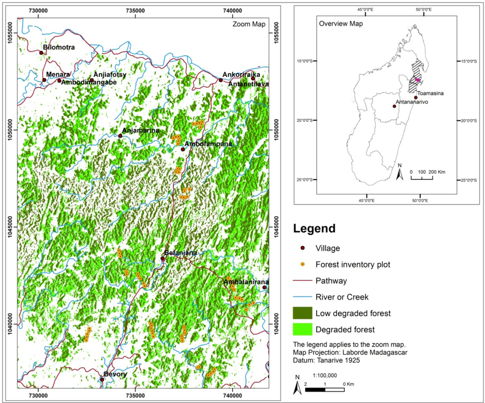
The study area is situated in the northeast of Madagascar, 200 km northwest of Toamasina, in the Soanierana Ivongo District of Analanjirofo Region (16°39′59″S/49°35′00″E). Topographically the area is characterized by a hilly landscape. Rainfall is very abundant, occurring on average on 224 days a year, and totaling up to 3,677 mm annually. Humidity generally reaches 75%, and the average temperature in the area is 23.7 °C. The location of the study area is illustrated in Figure 1, with a forest type classification and the location of the forest inventory plots shown in the close-up.
This forest area is part of an important ecological corridor situated between three protected forest areas: (a) Mananara Nord in the northeast, (b) Ambatovaky in the southwest, and (c) Pointe Larrée in the southeast.
The primary vegetation of this region is included in the “lowland rainforest” categories [14] in the Anthostema and MYRISTICACEAE class [15]. It is characterized in particular by dense evergreen trees with a canopy exceeding 30 m in height. The main threat to the lowland rainforest is from subsistence agriculture—through slash-and-burn activities, locally called “tavy”—and from illegal logging, which are the main causes of deforestation and degradation of the primary vegetation [16–20]. Consequently, the forests can be categorized into three forest degradation and disturbance classes as well as a fourth class consisting of other formations and non-forest as described in Table 1.
3. Materials and Methods
2.1. Field Data
Field data were collected in early 2009. All plots were selected randomly for the two forest strata. Their location was measured by a handheld GPS device. GPS data were post-processed, resulting in a horizontal accuracy of 10–15 m. In order to minimize erroneous effects on the results due to positioning errors, the 10 m × 50 m plots were selected based on the criterion that the surrounding forest vegetation within at least 10 m distance from the plot was the same as within the plot.
Aboveground biomass data were collected and obtained by applying stratified random sampling, followed by the calculation of allometric equations based on sample extraction calculation from the field. In this way, wood density was derived from branch density extrapolation using randomized branch sampling [21,22]. Wood density and the weight of the leaves were measured after drying at 70 °C until the weight no longer changed. Biomass was calculated using the forest type (model II) developed by Chave et al. [23]. In addition, the biomass values were validated using the international equations developed by Brown [24], adapted for humid areas (1,500 mm < P < 4,000 mm).
The biomass inventory was carried out for a total of 96 plots, including 48 plots of non-degraded forest and 48 plots of degraded forest. Each plot (10 m × 50 m) consisted of five subplots (10 m × 10 m). Each of these was subdivided into three compartments of different sizes, in which trees of different diameters were inventoried [25]. In compartment A (10 m × 10 m) all trees with dA > 20 cm were inventoried, in compartment B (5 m × 5 m) all trees with 5 cm < dB < 20 cm, and in compartment C (2.5 m × 2.5 m) all trees with dC < 5 cm. The dendrometric characteristics of each tree were recorded as: total height ht, bole height hB, length of the crown lc, diameter at 1.30 m height d1.30, and basal diameter for small trees db.
In order to generate regressions for the allometric equations, biomass samples for the two strata were collected. For this purpose, two macroplots of 100 m × 100 m were randomly selected in the study area, and samples were measured within subplots of 10 m × 10 m situated in each corner of each macroplot.
To ensure representativeness, 128 trees were randomly chosen in each subplot for the biomass modeling: 64 trees each for the two stratification classes (degraded forest and low-degraded forest). These trees were measured and then subdivided into four diameter size classes as follows: (1) d1.30 ≤ 10 cm; (2) 10 cm < d1.30 ≤ 20 cm; (3) 20 cm < d1.30 ≤ 30 cm); and (4) d1.30 > 30 cm. Additionally, for every tree, three biomass subpools—branch, bole, and crown—were considered for the volume calculation:
where:
- VB: volume of bole
- d1.30 : diameter at 1.30 m height (diameter at breast height, DBH)
- hB : height of bole
- Vb : volume of branch
- db : diameter of branch
- Lb : length of branch
- Vc : volume of crown
- hc : height of crown
- Lc : length of crown
Total biomass for each tree was calculated by summarizing all subpool volumes multiplied with their specific subpool mean density (for the bole: 0.60 t/m3, for the branch: 0.58 t/m3, and for the crown: 0.000346 t/m3). The resulting biomass values for each tree were then correlated with its measured DBH and height values in order to develop regression models with strong relationships. The highest R2 (0.978) was obtained with the following allometric equation:
where:
- Y: biomass of a tree [kg]
- d1.30: diameter at 1.30 m height [cm]
This formula was used to calculate biomass. For the calculation of carbon, biomass was multiplied with a conversion factor of 0.5, which is the default factor recommended by the International Panel on Climate Change (IPCC) [28].
The statistics of both parameters are listed in Table 2. More details on the species composition in the sample plots, the determination of biomass and carbon, and the corresponding statistical analysis can be found in Rakotondrasoa [26].
Due to a partial cloud and thick haze cover in the WorldView-2 satellite data, only a reduced sample size of 42 plots was available for this study. Of these plots, 25 are situated on flat areas and gently inclined slopes up to 6°, 14 are on slopes between 6° and 10°, and three are on steep slopes of around 20°.
2.2. Satellite Data and Preprocessing
The optical satellite sensor WorldView-2 was launched in October 2009. The sensor provides panchromatic data at a geometric resolution of 0.5 m, as well as multispectral data divided into eight spectral bands at a geometric resolution of 0.2 m. The spectral ranges of the eight bands are 0.40–0.45 μm (band 1-coastal blue), 0.45–0.51 μm (band 2-blue), 0.51–0.58 μm (band 3-green), 0.585–0.625 μm (band 4-yellow), 0.63–0.69 μm (band 5-red), 0.705–0.745 μm (band 6-red edge), 0.77–0.895 μm (band 7-near-infrared1), and 0.86–1.04 μm (band 8-near-infrared2).
The satellite data were delivered in product level LV3D, meaning that the data had been sensor-corrected, radiometrically corrected, and orthorectified. It was acquired with a mean in-track and cross-track viewing angle of 7.3° and 17.1° respectively, and a sun azimuth and sun elevation angle of 111.1° and 66.8°.
According to DigitalGlobe [29], the geolocation accuracy of the delivered image data ranges from 4.6 m to 10.7 m (CE90). This was checked by comparing the data to a georeferenced SPOT 5 dataset with a geometric resolution and accuracy of 5 m. The two datasets are in good agreement. Consequently, the horizontal accuracy of the WorldView-2 dataset is about 5 m–10 m.
Digital numbers were converted to top-of-atmosphere reflectance using the absolute radiometric calibration factors and effective bandwidths for each band, according to the formulas and directions provided by the satellite data provider DigitalGlobe [30]. The WorldView-2 data were then atmospherically corrected in order to reduce haze as well as other atmospheric and solar illumination influences. This was done using ATCOR 2, a procedure developed by Richter [31], which is capable of handling horizontally varying optical depths and contains a statistical haze removal algorithm. A radiative transfer code is required to compute the atmospheric transmittance, direct and diffuse solar flux, and path radiance. These quantities are summarized as atmospheric correction functions and had been previously calculated using the MODTRAN 4 code for several sensors, including WorldView-2.
Topographic correction was tested with the only available digital surface model (DSM) for the area, the Shuttle Radar Topography Mission (SRTM) DSM. It has a horizontal resolution of 90 m, which is insufficient for correcting topography of a WorldView-2 dataset with a horizontal resolution of 2 m. Nevertheless, the SRTM DSM was re-sampled step by step from 90 m to 45 m, from 45 m to 30 m, from 30 m to 15 m, from 15 m to 5 m, and from 5 m to the required resolution of 2 m. Besides the coarse resolution, a slight positional shift between the SRTM DSM and the WorldView-2 dataset was observed. After topographic correction, the consequences of this shift, combined with the coarse resolution, led to a chessboard pattern as well as a slightly shifted correction near ridges and summits. Differences between topographically corrected and uncorrected single band and vegetation index values for each plot were analyzed but proved to be very small. For this reason, it was decided to neglect topographic correction in order not to introduce an additional error to the reflectance values.
2.3. Simple Reflectance, Vegetation Indices, and Grey-level Co-occurrence (GLCM) Texture Measures
Preprocessing of a set of band ratios was followed by the calculation of vegetation indices, texture measures, and principal components. They were selected, based on previous research dealing with biomass and carbon estimations from optical satellite data [8,10,32,33]. GLCM texture measures were calculated for five different window sizes ranging from 15 × 15 to 23 × 23 pixels. The window sizes were determined after initial correlation tests on a small subset area. Considering the pixel size of 2.0 m, average window sizes were selected. In this way, shadow structures caused by trees are retained; ideally, these shadow structures differ between the two forest strata due to their specific characteristics, as described in Table 1.
WorldView-2 provides two bands in the near-infrared range of the electromagnetic spectrum: bands 7 and 8. Vegetation indices and ratios were calculated using each of the two near-infrared bands. For example, NDVI1 refers to NDVI, calculated using band 7 (NIR1), and NDVI2 refers to NDVI, calculated using band 8 (NIR2).
The mean value of all calculated parameters based on WorldView-2 data was derived for each of the 42 plots sized 10 m × 50 m. All derived parameters that were related to the field plot data are listed in Table 3.
2.4. Statistical Analysis
The relationships between biomass, carbon, and the computed mean value of each parameter per plot were analyzed using Pearson’s correlation, as well as stepwise multiple linear regression. The analysis included the available 20 plots representing the non-degraded forest stratum and 22 plots representing the degraded forest stratum. Bootstrap sampling was performed in order to account for the rather small sample sizes (see Tables A1–A8 of supplementary). The statistical parameters: R2, adjusted R2, p-level for the model, and root mean square error (RMSE) were calculated to ensure that the analysis would yield the best-fitting models for the two forest strata. Multicollinearity and overfitting indicators, Tolerance and Variance Inflation Factor (VIF), were taken into account as well.
3. Results
Since carbon was derived from the biomass data by multiplying it by a conversion factor of 0.5, all subsequent correlation and R2 results apply to both biomass and carbon.
3.1. Relationships between Biomass/Carbon and Parameters Derived from WorldView-2 Data
For the non-degraded forest stratum, Pearson’s correlation between biomass/carbon and parameters derived from WorldView-2 data resulted in one parameter with a significant coefficient: EVI2, with R2 = 0.413 (p = 0.01). Moderate correlations (p = 0.05) resulted for EVI1, band 6 (red edge), band 7 (NIR1), and band 8 (NIR2), as well as PC1 and PC2, and the textural measure Correlation of band 2 (blue) with a window size of 23 × 23 pixels.
For the degraded forest stratum, several texture measures correlated significantly: Correlation of band 5 (red), Mean of band 3 (green), Mean of band 4 (yellow), and particularly Mean of band 6 (red edge), Mean of band 7 (NIR1), and Mean of band 8 (NIR2). The smallest selected window size of 15 × 15 pixels achieved highest correlation coefficients, and correlations weakened with increasing window sizes. Pearson’s correlation coefficients between biomass/carbon and the spectral and textural parameters are listed in Table 4.
3.2. Stepwise Multiple Linear Regression Modeling
Stepwise multiple linear regression models were calculated using biomass and carbon as the dependent variables and all other parameters as the independent variables. The models that fulfill the collinearity requirements with a Tolerance value of >0.1 and a VIF value for all variables <10 [8] are presented in Tables 5 and 6.
For the non-degraded forest stratum, five models fulfill the statistical collinearity requirements. Using the most strongly correlating parameter, the vegetation index EVI2, a model was developed that explains 38% of the variability of measured biomass and carbon. It achieves a relative RMSE of 21.7% for both biomass and carbon, which corresponds to an absolute RMSE of 128 t/ha for biomass and 64 t/ha of carbon. The inclusion of four additional textural parameters led to an increase in the adjusted R2 to 0.816. In particular, the texture measures Variance of band 7 (NIR1), Variance of band 1 (coastal blue), Mean of band 8 (NIR2), and Correlation of band 5 (red), all with large window sizes of 21 × 21 as well as 23 × 23 pixels, led to a continuous improvement of the models. The absolute RMSE was reduced to 70 t/ha for biomass and 35 t/ha for carbon. This corresponds to a relative RMSE of 11.8%.
Three models were developed for the degraded forest stratum. They are based on the three texture measures: Correlation, Angular Second Moment, and Contrast, all derived from band 5 (red). The model using only one parameter, Correlation, achieved a relative RMSE of 11.3% for both biomass and carbon, which corresponds to an absolute RMSE of 52 t/ha for biomass and 26 t/ha of carbon. Up to 84.3% of the field data variability can be explained with a model including two additional variables, Angular Second Moment and Contrast, resulting in a absolute RMSE of 32 t/ha for biomass and an absolute RMSE of 16 t/ha for carbon. This corresponds to a relative RMSE of 6.8%. Looking at the window sizes of the texture measures, the strongest correlation was found for the smallest window size of 15 × 15 pixels. Parameters with larger window sizes of 21 × 21 and 23 × 23 pixels were also selected for the best-fitting models.
The 1:1 relationships between observed and modeled biomass values for the two strata and all developed models fulfilling the statistical requirements are illustrated in Figures 2 and 3.
Figure 2 shows the relationships between the modeled and the observed biomass values for the non-degraded forest stratum. The simple linear model based on EVI modeling non-degraded forest biomass (Model 1) yielded moderate results, overestimating the two lowest biomass values (plots 14 and 23). The middle-range biomass values were well-modeled, with moderate errors. The highest two biomass values were both underestimated (plots 2 and 38). With Model 2, adding the GLCM texture measure Variance of band 7 (NIR1), most plots tended to be overestimated, but with less outliers. Model 3, which included the additional GLCM texture measure Variance of band 1 (coastal blue), tended to underestimate biomass, but with a decreasing error. With Model 4 and Model 5, over- and under-estimations were balanced for plots with low and high biomass values.
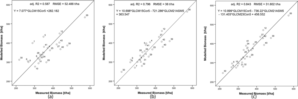
Figure 3 shows the relationship between the modeled and the measured biomass values for degraded forest. Model 1 based on the GLCM texture measure Correlation of band 5 (red) led to a well-balanced model with only few plots for which biomass was overestimated (plots 30, 7, 5) or underestimated (plots 40, 39 and 29). The GLCM texture measures Angular Second Moment and Contrast—both, again, derived from band 5 (red)—led to further improvements in Model 2 and Model 3, respectively.
4. Discussion
The objective of this study was to link biomass and carbon inventory data to WorldView-2 data and to analyze their relationships and the potential of WorldView-2 data for improved biomass and carbon estimation for two important strata of tropical rainforest. Models based on spectral and textural information were developed to estimate dry biomass and carbon. Pearson’s correlation revealed that (a) texture measures correlate more with biomass and carbon than spectral parameters, and (b) correlations are stronger for degraded forest than for non-degraded forest. The relative RMSE of the best models developed for each forest stratum are low, compared to results of other studies, and are thus promising.
Nevertheless, some critical points need to be addressed. The sample size of this study was limited, which is critical, but occurs frequently in the development of remote sensing-based biomass estimation models [5], particularly for areas that are difficult to access. The humid lowland rainforest with its dense vegetation is difficult to cross, which makes data collection extremely costly in terms of labor, time, and financial means. Unfortunately, the cloud cover in the satellite data further reduced the amount of usable samples in this study. Nevertheless, 42 sample plots were successfully linked to the satellite data, and the established relationships can serve as valuable information for future research on relating forest inventory data for humid rainforest to satellite data.
Linking field data to satellite data requires accurate preprocessing of all datasets. The positional error of the forest inventory plots and the satellite data must be minimal to ensure correspondence. During field work, the horizontal positioning error caused by the GPS when delineating field plots was kept within 10–15 m. The horizontal accuracy of the WorldView-2 data is within 5–10 m, according to DigitalGlobe [29]. In order to prevent errors caused by added positional errors of both datasets, only homogeneous forest areas of about 20 m × 60 m were considered for the establishment of the 10 m × 50 m plots.
Another critical point is the topographic and atmospheric correction of the dataset. An atmospheric correction was applied to reduce the influences of haze and illumination. However, the influence of slope and aspect due to changing topography might additionally affect vegetation reflectance. Almost two-thirds of the plots in the study area are on flat or slightly inclined slopes, whereas one third of the plots are on inclined or steep slopes, facing all directions. In a preliminary test, the WorldView-2 dataset was topographically corrected with the only available DSM, despite its coarse resolution of 90 m. The correlation of pre- and post-corrected data revealed only small differences for the spectral parameters. On this basis, it was decided to perform the analysis using the topographically uncorrected satellite data.
Sun and sensor position at time of acquisition also has an influence on cast shadow and thus on image texture, and it may be argued that the relation between textural parameters and biomass might decrease if cast shadows are minimal due to specific viewing and illumination geometries. This should be considered before ordering satellite data. Further research is needed to understand the impact of changing viewing and illumination geometry on the analyzed relationships and forest types.
Overall, a stronger relationship was observed for the degraded forest stratum. The two forest strata vary in their complexity in terms of vertical distribution of live and dead biomass, leading to different amounts and distributions of cast shadow. This affects the texture and reflectance response of the satellite data [32]. Texture measures seem to capture the varying forest canopy structures of the two observed forest strata much better than spectral reflectance or band ratios, due to their sensitivity to the spatial aspects of canopy shadow. The more heterogeneous the forest canopy structure, the stronger the correlation with textural parameters. This is not only confirmed by the results of this study dealing with very high resolution satellite data, but was also observed by Sarker et al. [8] and Lu [7] when analyzing high resolution ALOS data and medium resolution Landsat TM data, respectively. Furthermore, vegetation indices often saturate in high-biomass areas [7,43] due to high reflectance, and they do not always correlate strongly with biomass and carbon.
It was also observed that if biomass of a specific forest stratum correlates with forest canopy structure, it also correlates strongly with spectral parameters. Conversely, if biomass does not correlate with forest canopy structure, its relationship with texture measures is stronger than with spectral parameters. This was also noted by Fuchs et al. [10] for Siberian tundra forest, by Leboeuf et al. [44] for boreal black spruce stands, and by Lu et al. [32] for mature moist forest and liana forest stands in the Brazilian Amazon basin. Consequently, in the case of Malagasy lowland rainforest, the relationship between biomass and forest canopy structure is stronger for degraded forest stands than for non-degraded forest stands.
The only vegetation index that had a strong relationship with biomass and carbon was EVI for non-degraded forest. This index was developed in particular to increase sensitivity to high-biomass regions [35]. The two first principal components, as well as band 6 (red edge), band 7 (NIR1), and band 8 (NIR2), correlated moderately with biomass and carbon for non-degraded forest stands. Although textural parameters did not correlate significantly with biomass and carbon, a variety of texture measures contributed to the estimation models developed in this study: Variance, Mean, and Correlation, derived from the newly-introduced coastal blue band 1, band 7 (NIR1), band 8 (NIR2), and band 5 (red).
For the degraded forest stratum, the texture measures Mean derived from band 3 (green), band 4 (yellow), band 6 (red edge), and bands 7 and 8 (both NIR bands), as well as Correlation derived from band 5 (red) indicate a strong relationship with biomass and carbon. Besides Correlation, Angular Second Moment and Contrast, both derived from band 5, also helped to improve the models.
Unfortunately, WorldView-2 does not acquire information in the middle-infrared (MIR) wavelength range of the electromagnetic spectrum as it is acquired by the Landsat satellite sensors TM, ETM+, ASTER, or SPOT5. Several studies concluded that the relationship between the MIR wavelength range and vegetation properties, including biomass, is even stronger than for the NIR region [32,33,45,46].
The relative RMSE of the models developed for both strata in this study are mostly smaller than the relative error results obtained in other studies on biomass estimation using optical satellite data under comparable conditions, in terms of forest types, biomass ranges, satellite data resolution, input parameters, validation data, and applied methodologies. Castillo-Santiago et al. [47] estimated biomass of tropical rainforest in Mexico using a combination of spectral and textural parameters derived from SPOT5 data with a spatial resolution of 10 m and multiple linear regression modeling, obtaining a relative RMSE of 21.2%. Sarker et al. [8] achieved an RMSE of 46.5 t/ha for tropical forest biomass in Hong Kong using only textural parameters derived from ALOS data, again with a spatial resolution of 10 m. Unfortunately, this study gives no information regarding the relative RMSE. Nonetheless, the RMSE obtained in Hong Kong is similar to that obtained in our study for the degraded forest stratum, which has comparable field plot biomass ranges.
For carbon, the absolute RMSE for the non-degraded forest stratum is similar to the absolute RMSE results obtained in a study by Foster et al. [48], with absolute RMSE of 59.1 t/ha and 74.4 t/ha for two test areas in Amazon rainforest in Bolivia, which were derived from hyperspectral Hyperion data with a spatial resolution of 30 m. Again, no relative RMSE values are given.
These first results on linking biomass and carbon inventory data for tropical humid rainforest with very high resolution WorldView-2 satellite data are promising. The inclusion of grey level co-occurrence texture measures, as well as the subdivision of the plots into successional strata, led to a reduction of relative RMSE and to an improvement in biomass and carbon estimation models for Malagasy lowland rainforest.
The results confirm that EVI is particularly suitable for applications designed for mapping and monitoring tropical rainforest. Furthermore, the red edge and the two near-infrared spectral bands proved to have the strongest direct relationships with the field data. Out of the generated texture measures, Angular Second Moment, Contrast, Correlation, Mean, and Variance performed well.
5. Conclusions
This study explored the potential of WorldView-2 data for biomass and carbon estimation of tropical humid rainforest. Pearson’s correlation and stepwise multiple linear regression were performed, and models based on spectral and textural information derived from the WorldView-2 dataset were developed. The following conclusions can be drawn:
- Texture measures seem to capture the varying forest canopy structures of the two observed forest strata much better than spectral reflectance or band ratios, except for the vegetation index EVI, which had a strong relationship with the biomass and carbon field data for non-degraded forest.
- A strong relationship was observed between the degraded forest stratum field data and the satellite data. The developed models consist of the texture measures: Correlation, Angular Second Moment, and Contrast, all derived from band 5. The best model for degraded forest achieves an adjusted R2 of 0.843 and a relative RMSE of 6.8% for biomass and carbon. Furthermore, the texture measures Mean derived from band 3 (green), band 4 (yellow), band 6 (red edge), and bands 7 and 8 (both NIR bands) indicate a strong relationship with biomass and carbon. The best model developed for degraded forest Ydeg can be written as follows:
- A slightly weaker relationship was observed between non-degraded forest stratum field data and the satellite data. EVI, using the second NIR band of the sensor, as well as Variance, Mean, and Correlation, derived from the newly-introduced coastal blue band, both NIR bands, and the red band, contributed to the best model (adjusted R2 = 0.816, relative RMSE = 11.8%). The best model developed for non-degraded forest Ylow can be written as follows:
- Estimation of tropical rainforest biomass/carbon based on very high resolution satellite data can be improved by (a) developing and applying forest stratum–specific models, and (b) including textural information in addition to spectral information.
- WorldView-2 data are a valuable data source for biomass estimation. In this study, the main asset of WorldView-2 proved to be the sensor’s additional spectral bands and the spatial resolution of 2.0 m. The main drawback of the sensor is the lack of a middle-infrared band. The panchromatic band with its very high spatial resolution of 0.5 m might provide important information regarding other forest parameters such as crown area, crown diameter, and DBH; however, this question was beyond the scope of this study and will have to be examined in the future.
The next research steps will include analyzing the linkages between larger samples of tropical forest biomass data and satellite data with the same or similar spectral and spatial characteristics to confirm the present results and test the robustness of the developed models. Influences of varying acquisition and illumination geometries of other satellite scenes on the RMSE will have to be analyzed as well. Finally, future research will also focus on the assessment of carbon stock stored in secondary formations.
Acknowledgments
The author would like to thank DigitalGlobe for providing the WorldView-2 data at no charge. The author would also like to thank the team around Gabrielle Lalanirina Rajoelison: Harifidy Rakoto Ratsimba and Lovanirina Olivia Rakotondrasoa of École Supérieure des Sciences Agronomiques, Département des Eaux et Forêts, Université d’Antananarivo, who performed field work and laboratory analysis. Without their untiring efforts and hard work to establish the biomass and carbon forest inventory, this study would not have been possible.
References
- UNEP-WCMC. The Linkages between Biodiversity and Climate Change Mitigation; UNEP-WCMC: London, UK, 2008. Available online: http://www.cbd.int/doc/meetings/cc/ahteg-bdcc-02-02/official/ahteg-bdcc-02-02-05-en.pdf (accessed on 25 March 2012).
- UNFCCC. Outcome of the Work of the Ad Hoc Working Group on Long-Term Cooperative Action under the Convention—Policy Approaches and Positive Incentives on Issues Relating to Reducing Emissions from Deforestation and Forest Degradation in Developing Countries; and the Role of Conservation, Sustainable Management of Forests and Enhancement of Forest Carbon Stocks in Developing Countries. Proceedings of UNFCCC COP 16, Cancun, Mexico, 29 November–10 December 2010.
- UNFCCC. Methodological Guidance for Activities Relating to Reducing Emissions from Deforestation and Forest Degradation and The role of Conservation, Sustainable Management of Forests and Enhancement of Forest Carbon Stocks in Developing Countries, Draft Decision/CP.15; Advanced unedited version,; UNFCCC: Bonn, Germany, 2009; Available online: http://unfccc.int/files/na/application/pdf/cop15_ddc_auv.pdf (accessed on 25 July 2011).
- Ecoreserve. What is the UN-REDD Programme; Ecoreserve: San Francisco, CA, USA, 2010. Available online: http://www.ecoreserve.org/2010/06/02/what-is-the-un-redd-programme-reducing-emissions-from-deforestation-and-forest-degradation-in-developing-countries/ (accessed on 20 February 2011).
- Lu, D. The potential and challenge of remote sensing-based biomass estimation. Int. J. Remote Sens 2006, 27, 1297–1328. [Google Scholar]
- Dong, J.; Kaufmann, R.K.; Myneni, R.B.; Tucker, C.J.; Kauppi, P.E.; Liski, J.; Buermann, W.; Alexeyev, V.; Hughes, M.K. Remote sensing estimates of boreal and temperate forest carbon pools, sources, and sinks. Remote Sens. Environ 2003, 84, 393–410. [Google Scholar]
- Lu, D. Aboveground biomass estimation using Landsat TM data in the Brazilian Amazon. Int. J. Remote Sens 2005, 26, 2509–2525. [Google Scholar]
- Sarker, L.R.; Nichol, J.E. Improved forest biomass estimates using ALOS AVNIR-2 texture indices. Remote Sens. Environ 2011, 115, 968–977. [Google Scholar]
- Nelson, R.F.; Kimes, D.S.; Salas, W.A.; Routhier, M. Secondary forest age and tropical forest biomass estimation using Thematic Mapper imagery. Bioscience 2000, 50, 419–431. [Google Scholar]
- Fuchs, H.; Magdon, P.; Kleinn, C.; Flessa, H. Estimating aboveground carbon in a catchment of the Siberian forest tundra: Combining satellite imagery and field inventory. Remote Sens. Environ 2009, 113, 518–531. [Google Scholar]
- Boyd, D.S.; Danson, F.M. Satellite remote sensing of forest resources: Three decades of research development. Progr. Phys. Geogr 2005, 29, 1–26. [Google Scholar]
- Tuominen, S.; Pekkarinen, A. Performance of different spectral and textural aerial photograph features in multi-source forest inventory. Remote Sens. Environ 2005, 94, 256–268. [Google Scholar]
- Eckert, S.; Rakoto Ratsomba, H.; Rakotondrasoa, L.O.; Rajoelison, L.G.; Ehrensperger, A. Deforestation and forest degradation monitoring and assessment of biomass and carbon stock of lowland rainforest in the Analjirofo region, Madagascar. For. Ecol. Manage 2010, 262, 1996–2007. [Google Scholar]
- White, F. The Vegetation of Africa, a Descriptive Memoire to Accompany UNESCO/AETFAT Vegetation Map of Africa; UNESCO: Paris, France, 1983. [Google Scholar]
- Humbert, H.; Cours-Darne, G. Carte Internationale du Tapis Végétal et des Conditions Écologiques; Travaux de la Section Scientifique et Technique, Institut Français: Pondichery, France, 1965; Volume 6, p. 162. [Google Scholar]
- Humbert, H. La Destruction d’une Flore Insulaire par le Feu. Principaux Aspects de la végétation à Madagascar. In Mémoires de L'Académie Malgache, Fascicule V; Pitot, G., Ed.; Tananarive, Madagascar, 1927. [Google Scholar]
- Rauh, W. Problems of Biological Conservation in Madagascar. In Plants and Islands; Bramweil, D., Ed.; Academic Press: London, UK, 1979; pp. 405–421. [Google Scholar]
- Jolly, A.; Jolly, R. Malagasy Economics and Conservation: A Tragedy without Villains. In Key Environments: Madagascar; Jolly, A., Oberlé, P., Roland, R., Eds.; Pergamon Press: Oxford, UK, 1984; pp. 211–217. [Google Scholar]
- Sussman, R.W.; Richard, A.F.; Ravelojaona, G. Madagascar: Current projects and problems in conservation. Primate Conserv 1985, 5, 53–59. [Google Scholar]
- Jenkins, M.D. Madagascar: An Environmental Profile; IUCN: Gland, Switzerland, 1987. [Google Scholar]
- Valentine, H.T.; Tritton, L.M.; Furnival, G.M. Subsampling trees for biomass, volume, or mineral content. For. Sci 1984, 30, 673–681. [Google Scholar]
- Gregoire, T.G.; Valentine, H.T.; Furnival, G.M. Sampling methods to estimate foliage and other characteristics of individual trees. Ecology 1995, 56, 1181–1194. [Google Scholar]
- Chave, J.; Andalo, C.; Brown, S.; Cairns, M.A.; Chambers, J.Q.; Eamus, D.; Fölster, H.; Fromard, F.; Higuchi, N.; Kira, T.; et al. Tree allometry and improved estimation of carbon stocks and balance in tropical forests. Oecologia 2005, 145, 87–99. [Google Scholar]
- Brown, S. Estimating Biomass and Biomass Change of Tropical Forests: A Primer; FAO Forestry Paper 134; FAO: Rome, Italy, 1997. [Google Scholar]
- Rajoelison, L.G. Méthodologie d’Analyse Sylvicole dans une Forêt Naturelle; Akon’ny Ala No. 8 ; Bulletin du Département des Eaux & Forêts de l’Ecole Supérieure des Sciences Agronomiques; Université d’Antananarivo: Antananarivo, Madagascar, 1992; pp. 9–19. [Google Scholar]
- Rakotondrasoa, L.O. Etude du Stock de Carbone de la Forêt de Manompana: Nord Est de Madagascar; Mémoire de Diplômes d’Etudes Approfondies; Ecole Supérieure des Sciences Agronomiques, Département des Eaux et Forêts, Université d’Antananarivo: Antananarivo, Madagascar, 2009. [Google Scholar]
- Rakoto Ratsimba, H.; Rajoelison, L.G.; Rakotondrasoa, L.O.; Eckert, S.; Hergarten, C.; Ehrensperger, A. Dégradation des Forêts et Stock de Carbone dans la Biomasse Epigée de la Forêt dens Humide de Manompana: Nord Est de Madagascar. Presented at the International Scientific Conference on Technologies for Development, Lausanne, Switzerland, 8–10 February 2010.
- Houghton, J.T.; Meira Filho, L.G.; Lim, B.; Treanton, K.; Mamaty, I.; Bonduki, Y.; Griggs, D.J.; Callender, B.A. (Eds.) IPCC Guidelines for National Greenhouse Gas Inventories Volume 3; Greenhouse Gas Inventory Reference Manual (Revised ed.); IPCC/UK Meteorological Office: Bracknell, UK, 1996.
- DigitalGlobe. WorldView-2 Datasheet; DigitalGlobe: Longmont, CO, USA, 2010. Available online: http://dgl.us.neolane.net/res/dgl/survey/_8bandchallenge_resources.jsp?deliveryId=&id= (accessed on 28 July 2011).
- DigitalGlobe. Radiometric Use of WorldView-2 Imagery; Technical Note;. DigitalGlobe: Longmont, CO, USA, 2010. Available online: http://dgl.us.neolane.net/res/dgl/survey/_8bandchallenge.jsp. (accessed on 16 March 2011).
- Richter, R. Atmospheric/Topographic Correction for Satellite Imagery (ATCOR-2/3 User Guide 7.0); DLR-IB 565-01/09; DLR: Wessling, Germany, 2009. [Google Scholar]
- Lu, D.; Mausel, P.; Brondizio, E.; Moran, E. Relationships between forest stand parameters and Landsat TM spectral responses in the Brazilian Amazon Basin. For. Ecol. Manage 2004, 198, 149–167. [Google Scholar]
- Eckert, S. A Contribution to Sustainable Forest Management in Patagonia: Object-Oriented Classification and Forest Parameter Extraction based on ASTER and Landsat ETM+ Data. University of Zurich, Zurich, Switzerland, 2005. [Google Scholar]
- Kaufman, YJ.; Tanré, D. Atmospherically resistant vegetation index (ARVI) for EOS-MODIS. IEEE Trans. Geosci. Remote Sens 1992, 30, 261–270. [Google Scholar]
- Huete, A.; Didan, K.; Miura, T.; Rodriguez, E.P.; Gao, X.; Ferreira, L.G. Overview of the radiometric and biophysical performance of the MODIS vegetation indices. Remote Sens. Environ 2002, 83, 195–213. [Google Scholar]
- Crippen, R.E. Calculating the vegetation index faster. Remote Sens. Environ 1990, 34, 71–73. [Google Scholar]
- Rouse, J.W.; Haas, R.H.; Schell, J.A.; Deering, D.W. Monitoring Vegetation Systems in the Great Plains with ERTS. Third ERTS Symposium, NASA SP-351; NASA: Washington, DC, USA, 1973; 1, pp. 309–317. [Google Scholar]
- Rondeaux, G.; Steven, M.; Baret, F. Optimation of soil-adjusted vegetation indices. Remote Sens. Environ 1996, 55, 95–107. [Google Scholar]
- Richards, J.A. Remote Sensing Digital Image Analysis: An Introduction; Springer-Verlag: Berlin, Germany, 1999; p. 240. [Google Scholar]
- Jordan, C.F. Derivation of leaf area index from quality of light on the floor. Ecology 1969, 50, 663–666. [Google Scholar]
- Kanemasu, E.T. Seasonal canopy reflectance patterns of wheat, sorghum, and soybean. Remote Sens. Environ 1974, 3, 43–47. [Google Scholar]
- Haralick, R.M.; Shanmugan, K.; Dinstein, I. Textural features for image classification. IEEE Trans. Syst. Man Cybern 1973, 3, 610–621. [Google Scholar]
- Huete, A.R.; Liu, H.Q.; Van Leeuwen, W.J.D. The Use of Vegetation Indices in Forested Regions: Issues of Linearity and Saturation. Proceedings of 1997 IEEE International Geoscience and Remote Sensing Symposium, Noordwijk, The Nederlands, 3–8 August 1997; pp. 1966–1968.
- Leboeuf, A.; Beaudoin, A.; Forunier, R.A.; Guindon, L.; Luther, J.E.; Lambert, M.C. A shadow fraction method for mapping biomass of northern boreal black spruce forests using Quickbird imagery. Remote Sens. Environ 2007, 110, 488–500. [Google Scholar]
- Steininger, M.K. Satellite estimation of tropical secondary forest above-ground biomass: Data from Brazil and Bolivia. Int. J. Remote Sens 2000, 21, 1139–1157. [Google Scholar]
- Thenkabail, P.S.; Enclona, E.A.; Ashton, M.S.; Legg, C.; Jean De Dieu, M. Hyperion, IKONOS, ALI, and ETM+ sensors in the study of African rainforests. Remote Sens. Environ 2004, 90, 23–43. [Google Scholar]
- Castillo-Santiago, M.A.; Ricker, M.; De Jong, B.H.J. Estimation of tropical forest structure from SPOT-5 satellite images. Int. J. Remote Sens 2010, 31, 2767–2782. [Google Scholar]
- Foster, J.R.; Kingdon, C.C.; Townsend, P.A. Predicting Tropical Forest Carbon from EO-1 Hyperspectral Imagery in Noel Kempff Mercado National Park, Bolivia. Proceedings of 2002 IEEE International Geoscience and Remote Sensing Symposium, IGARSS ’02, Toronto, ON, Canada, 24–28 June 2002; 6, pp. 3108–3110.
Figure 1.
Overview and zoom map of the study area. The zoom map shows a forest classification, which was derived during an earlier study [13] from a SPOT 5 satellite image, acquired in 2009. The coverage of the WorldView-2 dataset coincides with the zoom map. The classification was not repeated based on the WorldView-2 satellite image. Additionally, as well as existing paths, the forest inventory also plots and indicates waterways and villages.

Figure 2.
Measured biomass vs. modeled biomass for non-degraded forest. Models 1–5 (a–e) were plotted indicating adjusted R2 and absolute RMSE. Each circle corresponds to a measurement plot. The diagonal represents the 1:1 relationship.
Figure 2.
Measured biomass vs. modeled biomass for non-degraded forest. Models 1–5 (a–e) were plotted indicating adjusted R2 and absolute RMSE. Each circle corresponds to a measurement plot. The diagonal represents the 1:1 relationship.

Figure 3.
Measured biomass vs. modeled biomass for degraded forest. Models 1–3 (a–c) were plotted indicating adjusted R2 and absolute RMSE. Each circle corresponds to a measurement plot. The diagonal represents the 1:1 relationship.
Figure 3.
Measured biomass vs. modeled biomass for degraded forest. Models 1–3 (a–c) were plotted indicating adjusted R2 and absolute RMSE. Each circle corresponds to a measurement plot. The diagonal represents the 1:1 relationship.


Table 1.
Characterization of forest degradation types present in the lowland rainforest in the study area.
| Class | Characterization | Photo |
|---|---|---|
| Non-degraded forest | Non-degraded forest with a very low level of disturbance. Contains a high carbon stock, close to a climax situation. Dense and closed canopy cover representing all types of typical plants (trees, palm trees, ferns). | 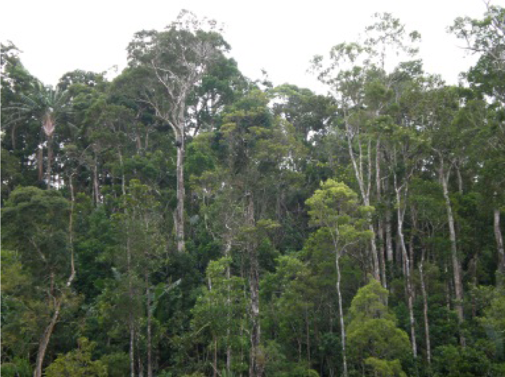 |
| Degraded forest | Degraded forest with a higher level of disturbance, but still with a high diversity and quantity of plants. Reduced carbon stock. Canopy cover is open. | 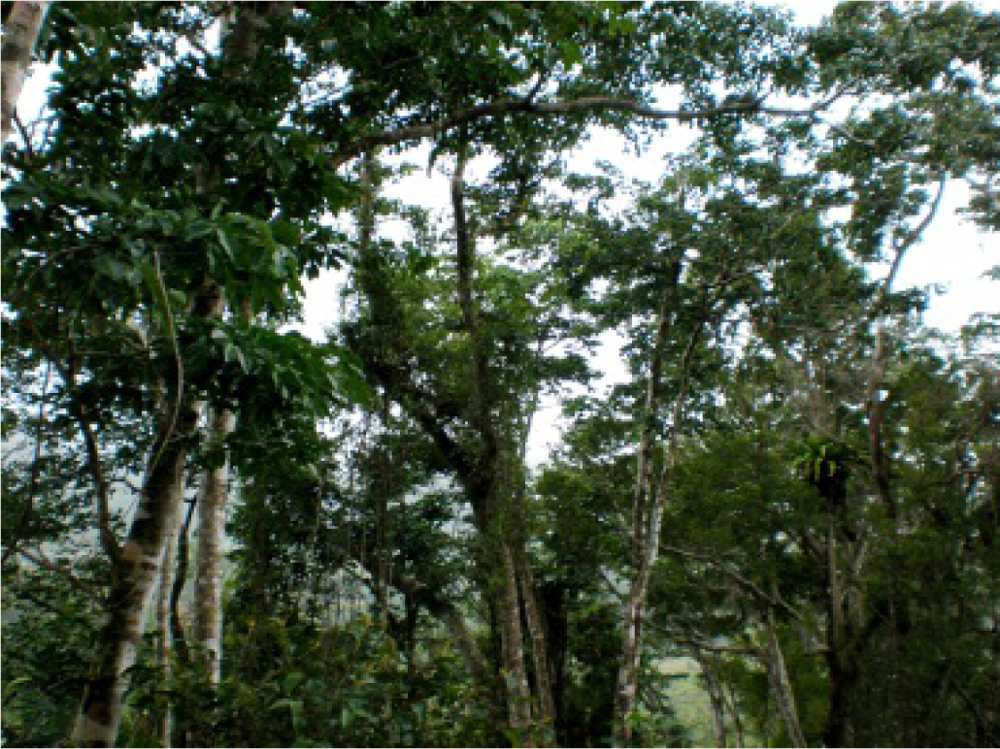 |
| Secondary formations | Vegetation regrowth after several disturbances of high intensity (generally regrowth after slash-and-burn activities) |  |
| Other formations and non-forest | Other formations, generally very highly degraded, with species such as Asplenium spp. indicating extreme degradation. A condition reached after frequent heavy disturbances of high intensity. |  |
| Parameter & Forest Stratum | No. | Min. | Max. | Mean | S.D. |
|---|---|---|---|---|---|
| Biomass, non-degraded | 20 | 323.304 | 1048.085 | 575.853 | 162.757 |
| Biomass, degraded | 22 | 217.165 | 572.223 | 359.572 | 79.727 |
| Carbon, non-degraded | 20 | 161.652 | 524.043 | 287.926 | 81.378 |
| Carbon, degraded | 22 | 108.583 | 286.112 | 179.786 | 39.863 |
| Parameter | Formula | References |
|---|---|---|
| Single bands | ||
| WorldView-2 bands 1–8 | ||
| Vegetation indices | ||
| ARVI | (NIR – 2 × RED + BLUE)/(NIR + 2 × RED – BLUE) | [34] |
| EVI | G × ((NIR – RED)/(NIR +C1 × RED – C2xBLUE + L)) | [35] |
| IPVI | NIR/(NIR + RED) | [36] |
| NDVI | (NIR – RED)/(NIR + RED) | [37] |
| OSAVI | (NIR – RED)/(NIR + RED + Y) | [38] |
| Image transform | ||
| Principal components 1–8 (PC1–PC8) | [39] | |
| Simple ratios | ||
| RVI | NIR/RED | [40] |
| NIR/GREEN | NIR/GREEN | |
| GRVI | GREEN/RED | [41] |
| GLCM texture measures (window sizes: 15 × 15 – 23 × 23 pixels) | ||
| [42] | ||
| Mean | ||
| Variance | ||
| Homogeneity | ||
| Contrast | ||
| Dissimilarity | ||
| Entropy | ||
| Angular Second Moment | ||
| Correlation | ||
ARVI: atmospherically resistant vegetation index; EVI: enhanced vegetation index, with G = 2.5, C1 = 6, C2 = 7.5, L = 1; IPVI: infrared percentage vegetation index; NDVI: normalized difference vegetation index; OSAVI: optimized soil-adjusted vegetation index, with Y = 0.16; RVI: ratio vegetation index; GRVI: green ratio vegetation index; NIR: near-infrared; NIR1: band 7; NIR2: band 8; BLUE: visible blue band; RED: visible red band; GREEN: visible green band.
Table 4.
Statistically significant Pearson’s correlation coefficients r and R2 for linear relationships between carbon/biomass and the derived spectral parameters from the WorldView-2 data as well as between carbon/biomass and the textural parameters. Spectral parameters are listed in the order of decreasing correlations; textural parameters are listed in the order of increasing window sizes.
| Stratum | Parameter | Pearson’s r | R2 |
|---|---|---|---|
| Non-degraded forest (n=20) | EVI 2 | 0.643** | 0.413 |
| EVI 1 | 0.531* | 0.282 | |
| PC 2 | 0.508* | 0.258 | |
| Band 8 | 0.499* | 0.249 | |
| Band 7 | 0.486* | 0.236 | |
| Band 6 | 0.480* | 0.230 | |
| PC 1 | 0.453* | 0.205 | |
| GLCM23 Correlation band 2 | 0.454* | 0.206 | |
| Degraded forest (n=22) | GLCM15 Correlation band 5 | 0.766** | 0.587 |
| GLCM15 Mean band 6 | 0.758** | 0.575 | |
| GLCM15 Mean band 8 | 0.723** | 0.523 | |
| GLCM15 Mean band 7 | 0.719** | 0.517 | |
| GLCM15 Mean band 4 | 0.614** | 0.377 | |
| GLCM15 Mean band 3 | 0.604** | 0.365 | |
| GLCM17 Correlation band 5 | 0.718** | 0.516 | |
| GLCM17 Mean band 6 | 0.754** | 0.569 | |
| GLCM17 Mean band 8 | 0.718** | 0.516 | |
| GLCM17 Mean band 7 | 0.714** | 0.510 | |
| GLCM17 Mean band 4 | 0.611** | 0.373 | |
| GLCM17 Mean band 3 | 0.601** | 0.361 | |
| GLCM19 Correlation band 5 | 0.637** | 0.406 | |
| GLCM19 Mean band 6 | 0.750** | 0.563 | |
| GLCM19 Mean band 8 | 0.713** | 0.508 | |
| GLCM19 Mean band 7 | 0.709** | 0.503 | |
| GLCM19 Mean band 4 | 0.608** | 0.370 | |
| GLCM19 Mean band 3 | 0.598** | 0.358 | |
| GLCM21 Correlation band 5 | 0.637** | 0.406 | |
| GLCM21 Mean band 6 | 0.750** | 0.563 | |
| GLCM21 Mean Band 8 | 0.713** | 0.508 | |
| GLCM21 Mean band 7 | 0.709** | 0.503 | |
| GLCM21 Mean band 4 | 0.608** | 0.370 | |
| GLCM21 Mean band 3 | 0.598** | 0.358 | |
| GLCM23 Correlation band 5 | 0.543** | 0.295 | |
| GLCM23 Mean band 6 | 0.746** | 0.557 | |
| GLCM23 Mean band 8 | 0.709** | 0.503 | |
| GLCM23 Mean band 7 | 0.705** | 0.497 | |
| GLCM23 Mean band 4 | 0.606** | 0.367 | |
| GLCM23 Mean band 3 | 0.596** | 0.355 |
**Correlation is significant at the 0.01 level.
*Correlation is significant at the 0.05 level.
| Model (non-degraded forest) (bootstrapping No. of samples) Variables | R2 | Adj. R2 | RMSE [t/ha] (Biomass) | RMSE [t/ha] (Carbon) | Relative RMSE [%] (Carbon/Biomass) | Tolerance (>0.1) | VIF (<10) |
|---|---|---|---|---|---|---|---|
| 1 (n = 30) | 0.413 | 0.381 | 128.08 | 64.04 | 21.74 | ||
| EVI2 | 1.000 | 1.000 | |||||
| 2 (n = 60) | 0.639 | 0.596 | 103.40 | 51.70 | 17.55 | ||
| EVI2 | 0.830 | 1.204 | |||||
| GLCM23 Variance band 7 | 0.830 | 1.204 | |||||
| 3 (n=100) | 0.746 | 0.699 | 89.30 | 44.65 | 15.16 | ||
| EVI2 | 0.826 | 1.210 | |||||
| GLCM23 Variance band 7 | 0.824 | 1.213 | |||||
| GLCM21 Variance band 1 | 0.980 | 1.021 | |||||
| 4 (n=150) | 0.812 | 0.762 | 79.41 | 39.71 | 13.48 | ||
| EVI2 | 0.826 | 1.211 | |||||
| GLCM23 Variance band 7 | 0.804 | 1.244 | |||||
| GLCM21 Variance band 1 | 0.971 | 1.030 | |||||
| GLCM23 Mean band 8 | 0.962 | 1.039 | |||||
| 5 (n=210) | 0.865 | 0.816 | 69.77 | 34.89 | 11.84 | ||
| EVI2 | 0.730 | 1.370 | |||||
| GLCM23 Variance band 7 | 0.742 | 1.349 | |||||
| GLCM21 Variance band 1 | 0.970 | 1.031 | |||||
| GLCM23 Mean band 8 | 0.782 | 1.279 | |||||
| GLCM23 Correlation band 5 | 0.597 | 1.675 | |||||
| Model (degraded forest) (bootstrapping no of samples) Variables | R2 | Adj. R2 | RMSE [t/ha] (Biomass) | RMSE [t/ha] (Carbon) | Relative RMSE [%] | Tolerance (>0.1) | VIF (<10) |
|---|---|---|---|---|---|---|---|
| 1 (n=30) | 0.587 | 0.567 | 52.49 | 26.24 | 11.33 | ||
| GLCM15 Correlation band 5 | 1.000 | 1.000 | |||||
| 2 (n=60) | |||||||
| GLCM15 Correlation band 5 | 0.816 | 0.796 | 36.00 | 18.00 | 7.77 | 0.598 | 1.673 |
| GLCM21 Angular Second Moment band 5 | 0.598 | 1.673 | |||||
| 3 (n=100) | 0.865 | 0.843 | 31.60 | 15.80 | 6.82 | ||
| GLCM15 Correlation band 5 | 0.594 | 1.683 | |||||
| GLCM21 Angular Second Moment band 5 | 0.596 | 1.676 | |||||
| GLCM23 Contrast band 5 | 0.994 | 1.006 | |||||
Share and Cite
MDPI and ACS Style
Eckert, S. Improved Forest Biomass and Carbon Estimations Using Texture Measures from WorldView-2 Satellite Data. Remote Sens. 2012, 4, 810-829. https://doi.org/10.3390/rs4040810
AMA Style
Eckert S. Improved Forest Biomass and Carbon Estimations Using Texture Measures from WorldView-2 Satellite Data. Remote Sensing. 2012; 4(4):810-829. https://doi.org/10.3390/rs4040810
Chicago/Turabian StyleEckert, Sandra. 2012. "Improved Forest Biomass and Carbon Estimations Using Texture Measures from WorldView-2 Satellite Data" Remote Sensing 4, no. 4: 810-829. https://doi.org/10.3390/rs4040810