Shoreline Change along Sheltered Coastlines: Insights from the Neuse River Estuary, NC, USA


Abstract
:1. Introduction

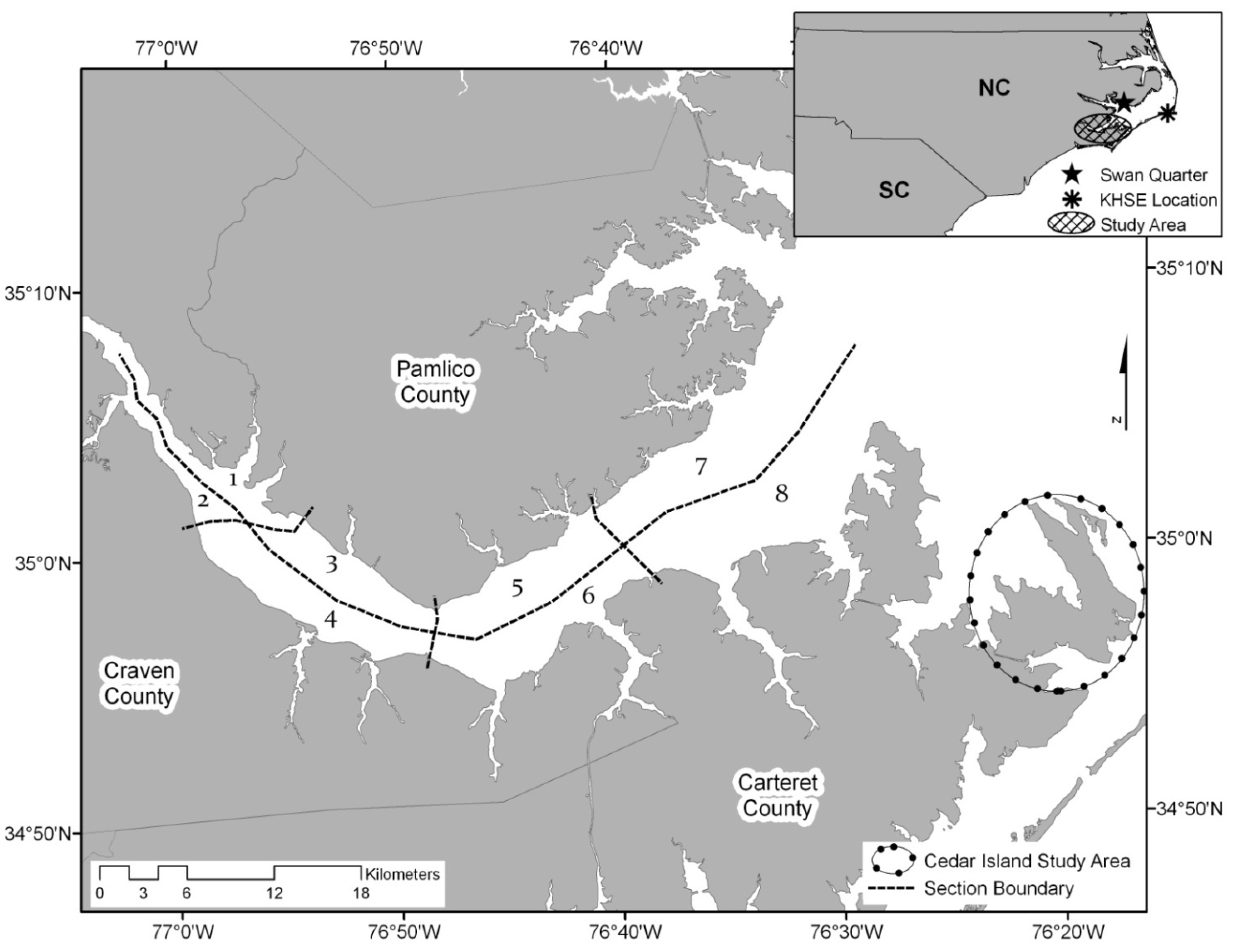
2. Study Area
3. Methods
3.1. Determining Shoreline Change Rates
3.2. Evaluating Parameters that Influence Shoreline-Change Rates
4. Results
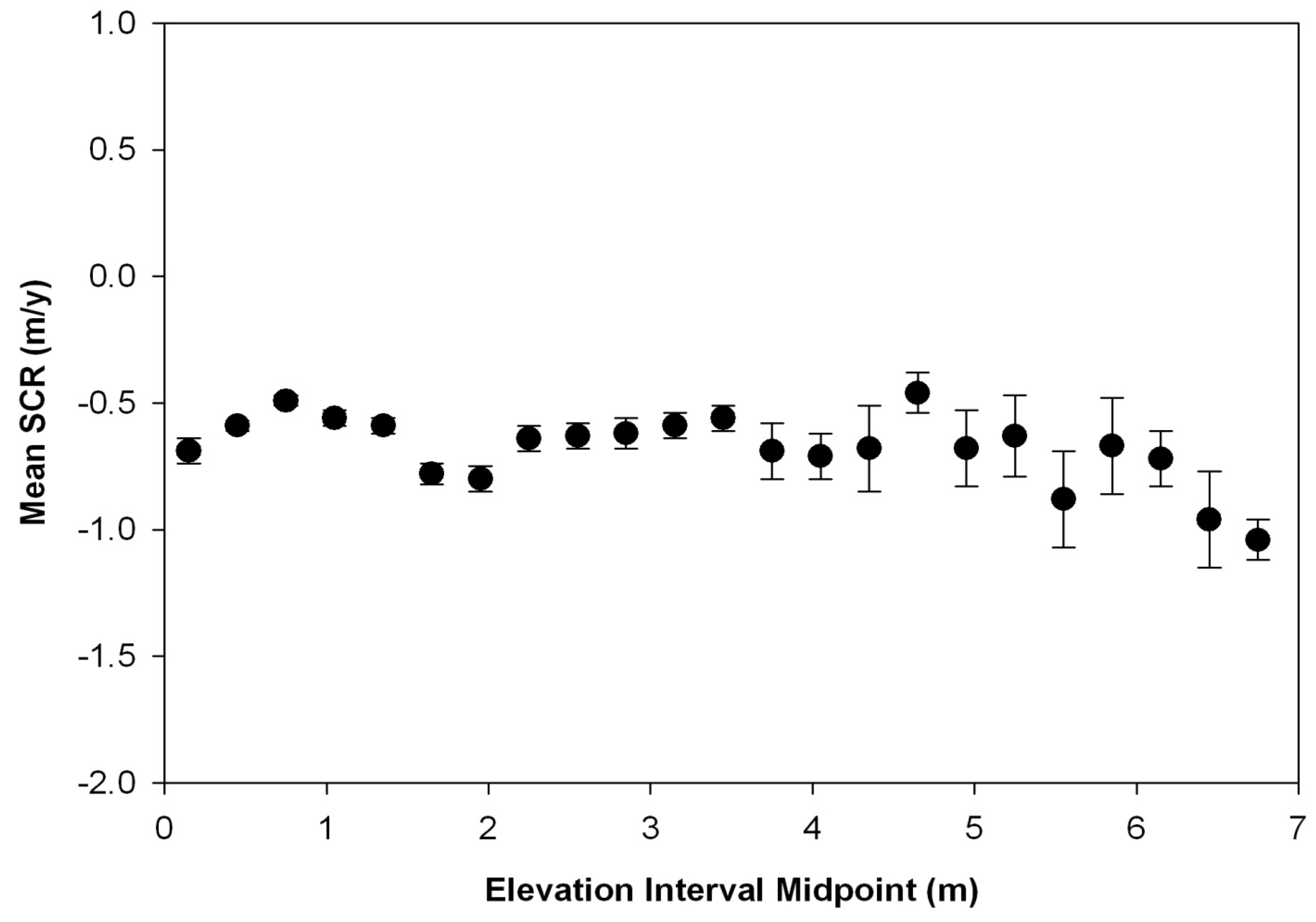
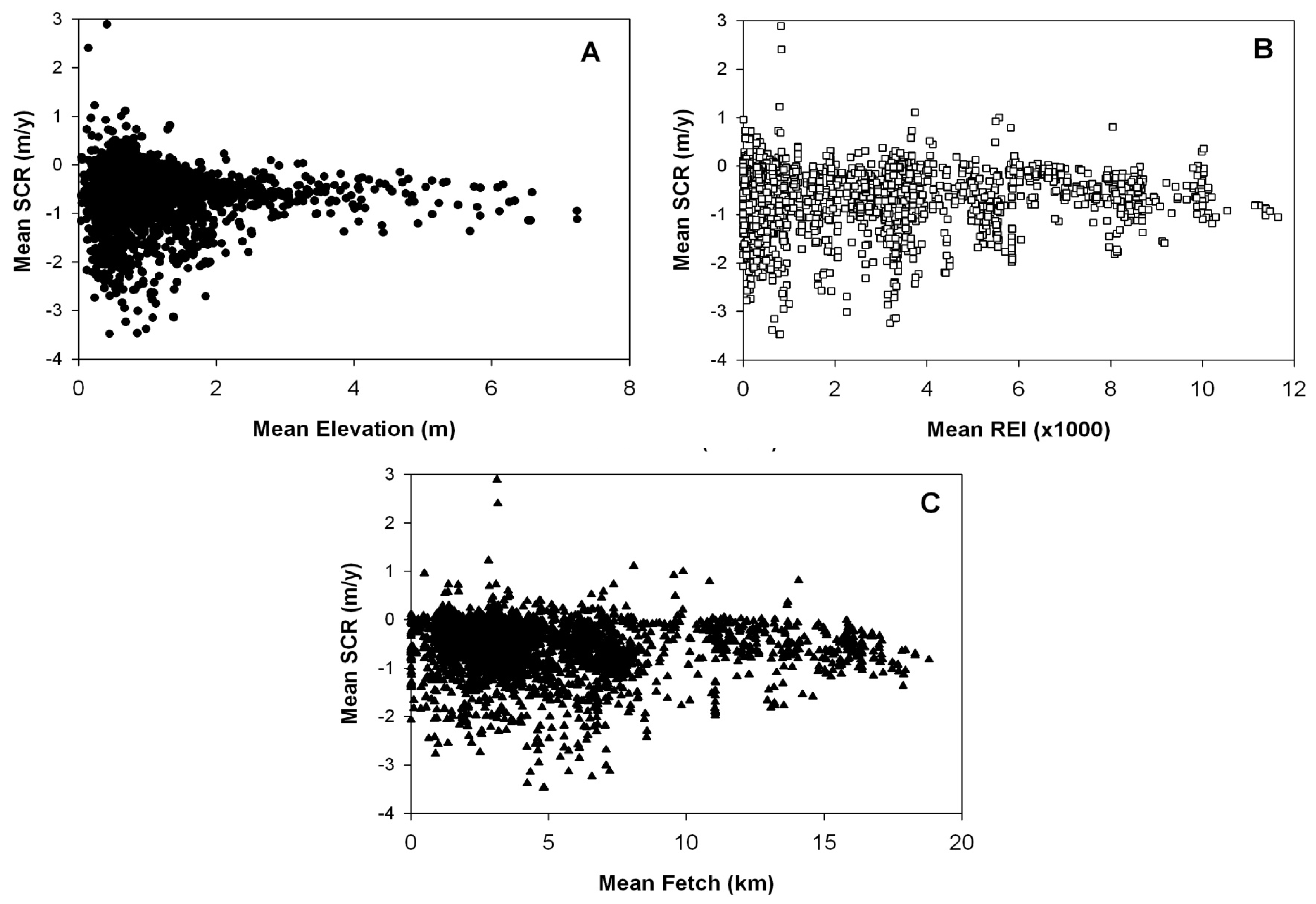
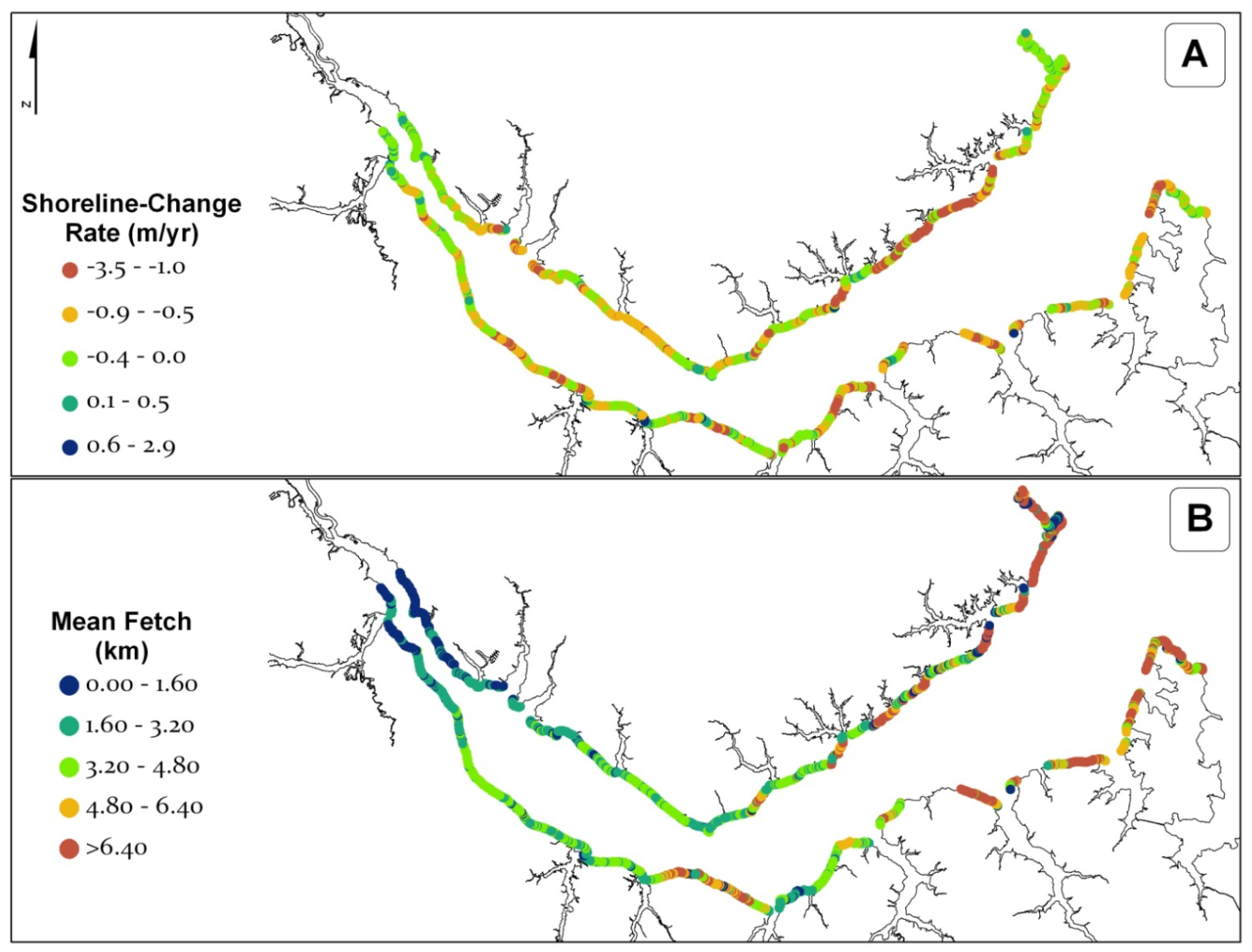
4.1. Regional Scale

| Parameter | Minimum | Maximum | Mean | Standard Deviation |
|---|---|---|---|---|
| Shoreline Change Rate (m yr−1) | −3.48 | 2.89 | −0.58 | 0.54 |
| Elevation (m) | 0.04 | 7.20 | 0.96 | 0.80 |
| Fetch(km) | East | 0 | 64.1 | 8.81 |
| Northeast | 0 | 100 | 7.51 | |
| North | 0 | 38.8 | 4.63 | |
| Northwest | 0 | 25.9 | 3.14 | |
| West | 0 | 19.0 | 2.47 | |
| Southwest | 0 | 22.6 | 1.82 | |
| South | 0 | 16.6 | 2.66 | |
| Mean Fetch (km) | 0 | 18.8 | 4.65 | 3.66 |
| Relative Exposure Index (103) | 0 | 11.6 | 1.82 | 2.51 |


| Parameter | LULC Category | ||||
|---|---|---|---|---|---|
| Wetland | Forest | Sediment Bank | Other | ||
| Mean | Shoreline Change Rate (m yr−1) | −0.53 † | −0.57 † | −0.70 ‡ | −0.56 † |
| Elevation (m) | 0.85 † | 1.40 ‡ | 1.09 # | 1.09 # | |
| Fetch (km) | 4.9 † | 3.5 ‡ | 4.6 † | 3.7 ‡ | |
| Relative Exposure Index (103) | 2.0 † | 1.0 ‡ | 1.7 †,# | 1.3 ‡,# | |
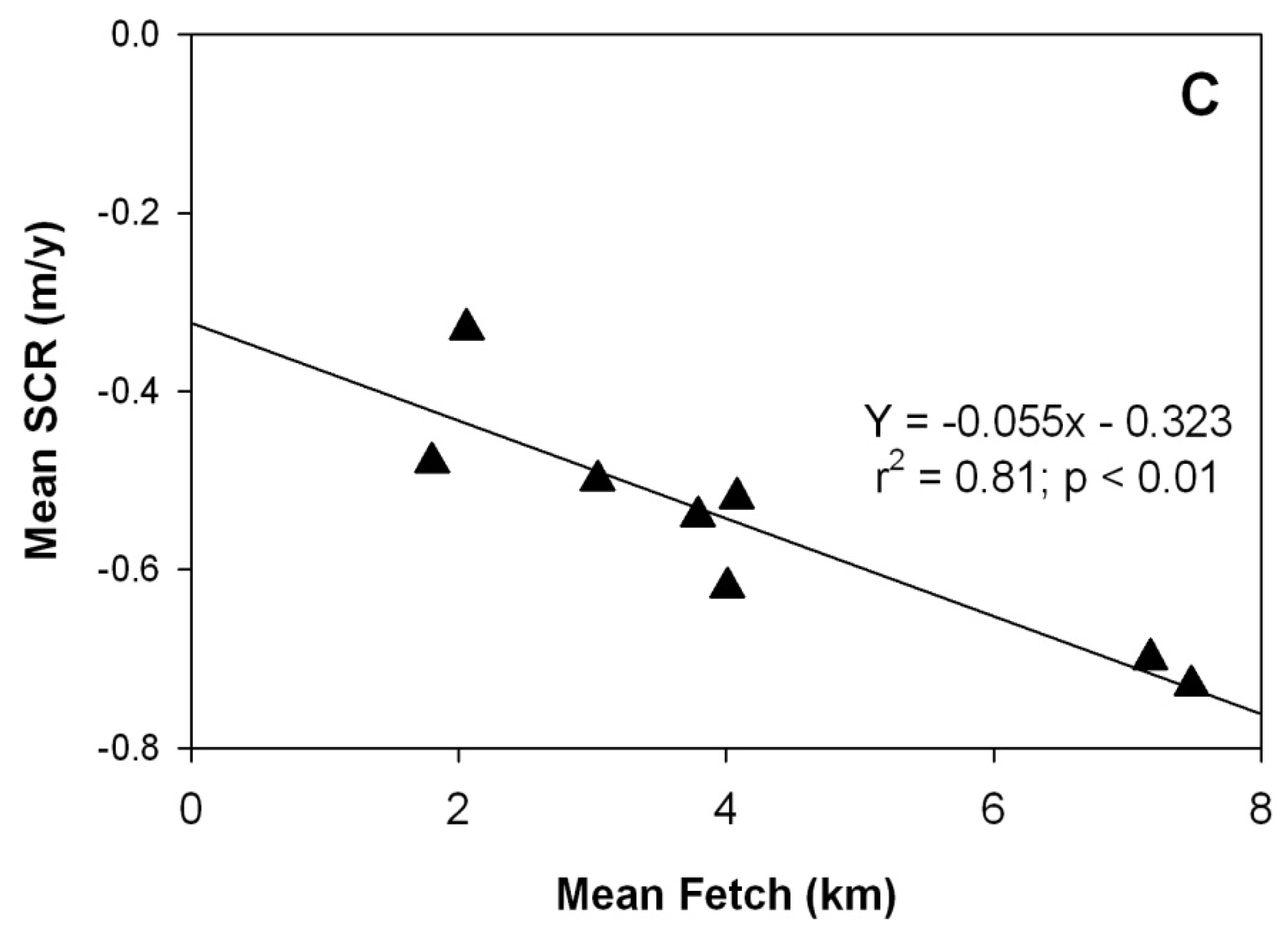
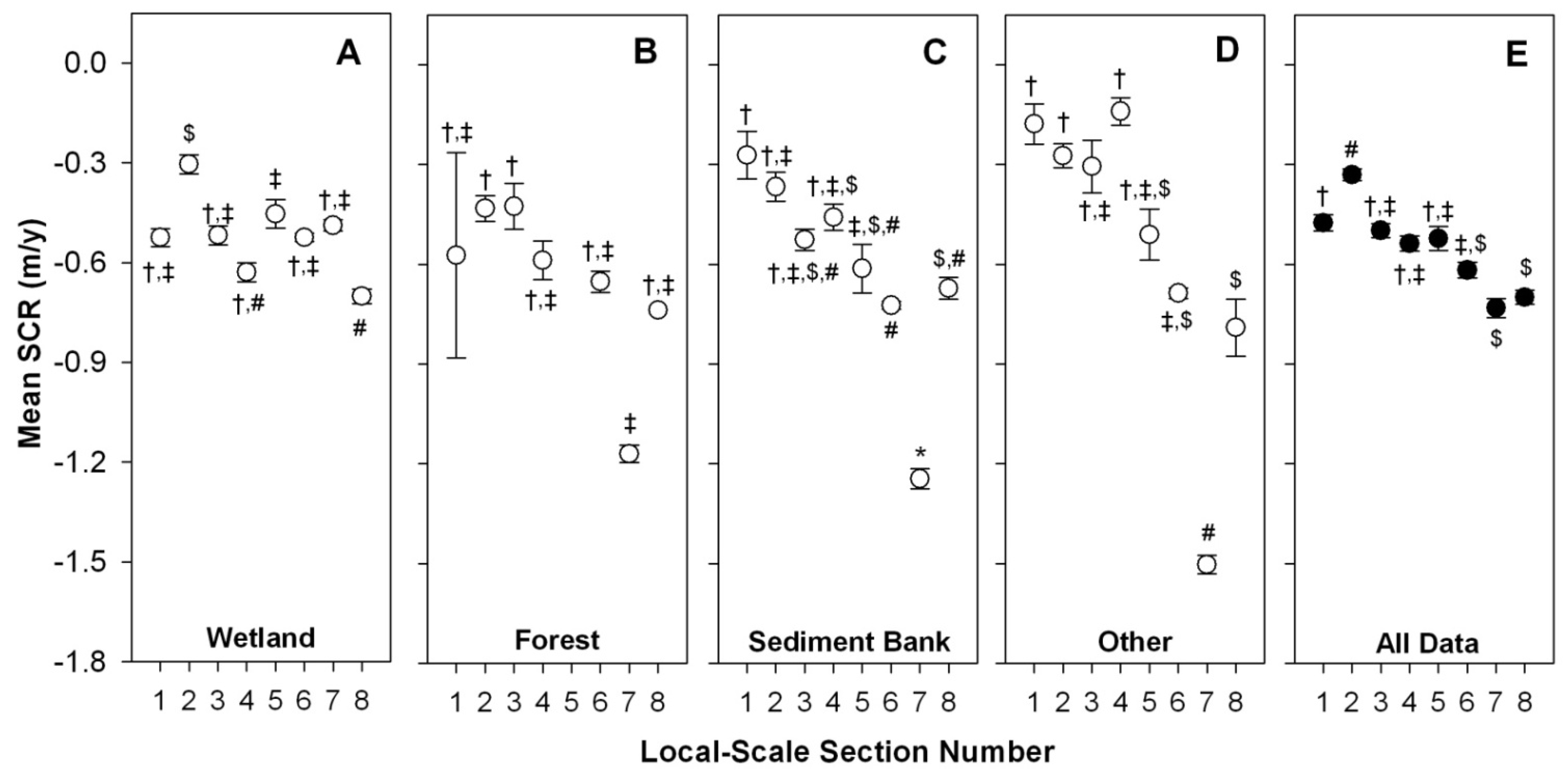
4.2. Local Scale
| Parameter | Local Section Number | ||||||||
|---|---|---|---|---|---|---|---|---|---|
| 1 | 2 | 3 | 4 | 5 | 6 | 7 | 8 | ||
| Mean | Shoreline Change Rate (m yr−1) | −0.48 † | −0.33 ‡ | −0.50 †,# | −0.54 †,# | −0.52 †,# | −0.62 #,$ | −0.73 $ | −0.70 $ |
| Elevation (m) | 0.62 † | 1.63 ‡ | 1.30 # | 1.51 ‡ | 1.00 $ | 0.90 $ | 0.64 † | 0.58 † | |
| Fetch (km) | 1.80 † | 2.06 † | 3.04 ‡ | 3.79 # | 4.08 # | 4.01# | 7.48 $ | 7.17 $ | |
| Relative Exposure Index (103) | 0.10 † | 0.13 † | 0.29 † | 0.78 ‡ | 1.11 ‡ | 1.65# | 3.71 $ | 4.03 $ | |
| Local Section | Land-Use Land-Cover Category | |||||||
| Wetland | Forest | Sediment Bank | Other | |||||
| SCR | (%) | SCR | (%) | SCR | (%) | SCR | (%) | |
| 1 | −0.52 | (82) | −0.57 | (1) | −0.27 | (11) | −0.18 | (6) |
| 2 | −0.30 †,‡ | (39) | −0.43 † | (16) | −0.37 †,‡ | (21) | −0.27 ‡ | (24) |
| 3 | −0.52 | (60) | −0.43 | (2) | −0.53 | (29) | −0.31 | (9) |
| 4 | −0.63 † | (44) | −0.59 † | (16) | −0.46 † | (35) | −0.14 ‡ | (5) |
| 5 | −0.45 | (44) | N/A | N/A | −0.61 | (36) | −0.51 | (20) |
| 6 | −0.52 | (47) | −0.65 | (10) | −0.72 | (31) | −0.69 | (11) |
| 7 | −0.49 † | (70) | −1.17 ‡ | (1) | −1.24 ‡ | (24) | −1.50 ‡ | (5) |
| 8 | −0.70 | (68) | −0.74 | (1) | −0.67 | (25) | −0.79 | (6) |

5. Discussion
5.1. Regional Scale Relationships
5.2. Local Scale Trends
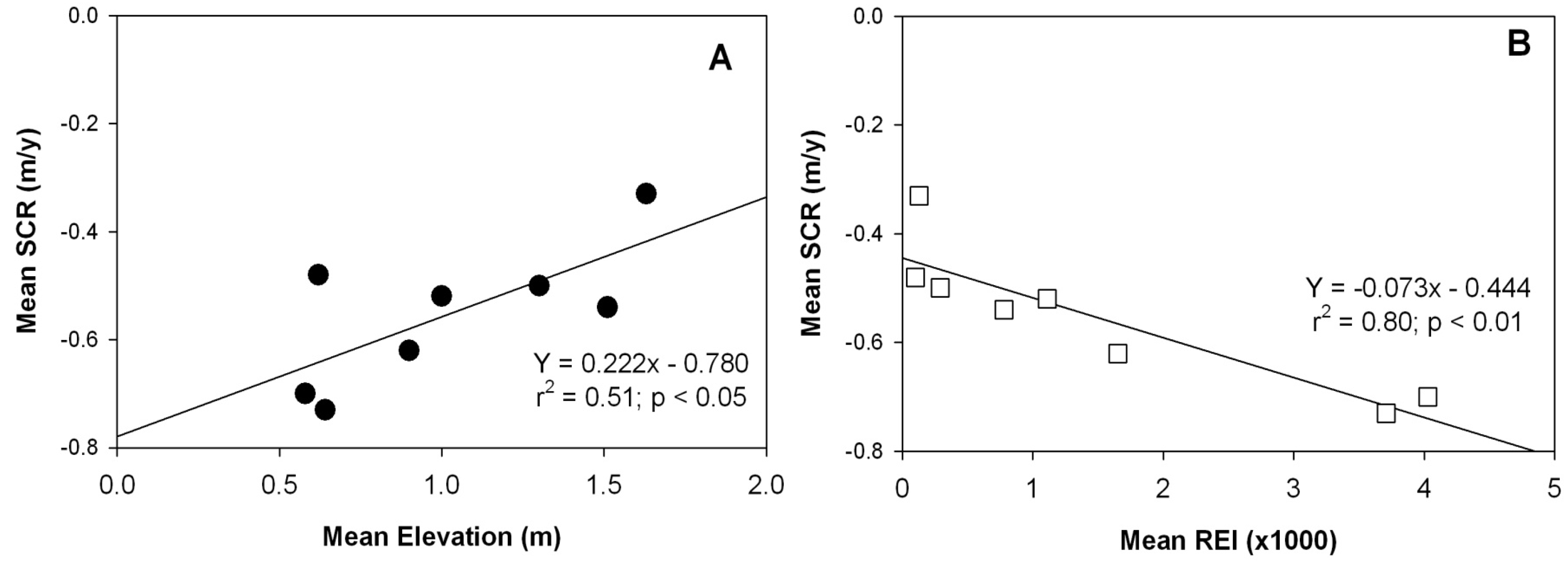
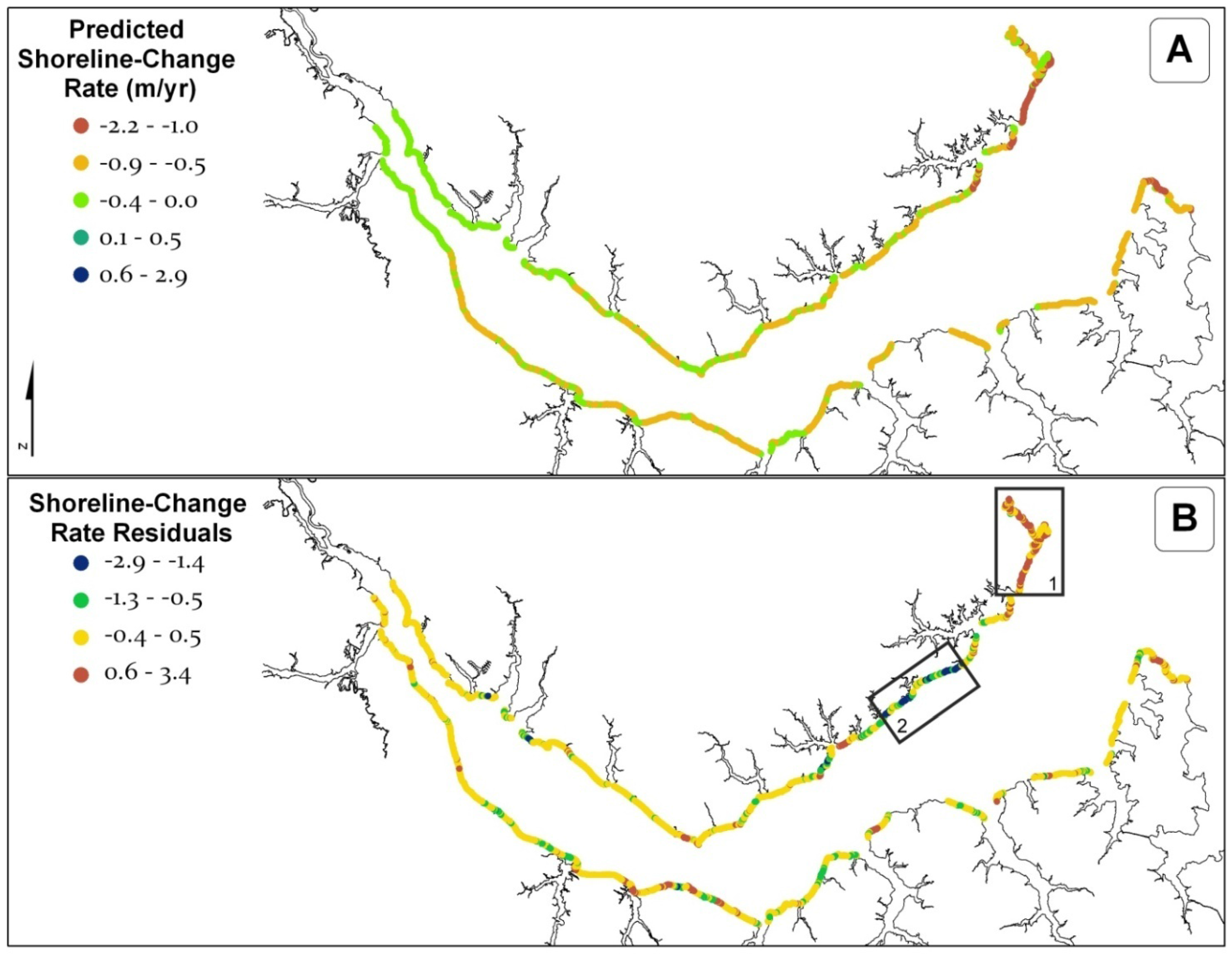
5.3. Predicting Erosion Rates
5.4. Additional Influences on Shoreline Change
6. Summary and Conclusions
Acknowledgments
References
- Martin, D.M.; Morton, T.; Dobrzynski, T.; Valentine, B. Estuaries on the Edge: The Vital Link Between Land and Sea; The American Oceans Campaign: Washington, DC, USA, 1996; p. 297. [Google Scholar]
- Crossett, K.M.; Culliton, T.J.; Wiley, P.C.; Goodspeed, T.R. Population Trends along the Coastal United States: 1980–2008; 2004. Available online: http://www.oceanservice.noaa.gov/programs/mb/pdfs/coastal_pop_trends_complete.pdf (accessed on 12 January 2011).
- Benoit, J.; Hardaway, C.S., Jr.; Hernansez, D.; Holman, R.; Koch, E.; McLellan, N.; Peterson, S.; Reed, D.; Suman, D. Mitigating Shore Erosion Along Sheltered Coasts; The National Academies Press: Washington, DC, USA, 2007. [Google Scholar]
- McNinch, J.E. Geologic control in the nearshore: Shore-oblique sandbars and shoreline erosional hotspots, Mid-Atlantic Bight, USA. Mar. Geol. 2004, 211, 121–141. [Google Scholar] [CrossRef]
- Miller, H.C. Field measurements of longshore sediment transport during storms. Coastal Eng. 1999, 36, 301–321. [Google Scholar] [CrossRef]
- Zhang, K.; Douglas, B.C.; Leatherman, S.P. Global warming and coastal erosion. Climate Change 2004, 64, 41–58. [Google Scholar] [CrossRef]
- Day, J.W.J.; Hall, C.A.S.; Kemp, W.M.; Yàñez-Arancibia, A. Estuarine Ecology; John Wiley & Sons, Inc.: New York, NY, USA, 1989; p. 258. [Google Scholar]
- Gibson, G. An Analysis of Shoreline Change at Little Lagoon, Alabama. M.Sc. Thesis, Department of Geography, Virginia Polytechnic Institute and State University, Blacksburg, VA, USA, 2006. [Google Scholar]
- Hennessee, E.L.; Halka, J.P. Hurricane Isabel and erosion of Chesapeake Bay shorelines, Maryland. In Hurricane Isabel in Perspective; Sellner, K.G., Ed.; Chesapeake Research Consortium: Edgwater, MD, USA, 2005; Volume 05-160, pp. 81–88. [Google Scholar]
- Phillips, J.D. Spatial Analysis of Shoreline Erosion, Delaware Bay, New Jersey. Ph.D. Dissertation, Department of Geography, Rutgers-The State University, New Brunswick, NJ, USA, 1985. [Google Scholar]
- Price, F.D. Quantification, Analysis, and Management of Intracoastal Waterway Channel Margin Erosion in the Guana Tolomato Matanzas National Estuarine Research Reserve, Florida; National Estuarine Research Reserve Technical Report Series 2006:1; National Estuarine Research Reserve: Apalachicola, FL, USA, 2006. [Google Scholar]
- Riggs, S.R. Shoreline Erosion in North Carolina Estuaries; Publication No. UNC-SG-01-11; North Carolina Sea Grant Raleigh: Raleigh, NC, USA, 2001. [Google Scholar]
- Riggs, S.R.; Ames, D.V. Drowning the North Carolina Coast: Sea Level Rise and Estuarine Dynamics; Publication No. UNC-SG-03-04; North Carolina Sea Grant Raleigh: Raleigh, NC, USA, 2003. [Google Scholar]
- Schwimmer, R.A. Rates and processes of marsh shoreline erosion in Rehoboth Bay, Delaware, USA. J. Coast. Res. 2001, 17, 672–683. [Google Scholar]
- Swisher, M.L. The Rates and Causes of Shore Erosion around a Transgressive Coastal Lagoon, Rehoboth Bay, Delaware. M.Sc. Thesis, College of Marine Studies, University of Delaware, Newark, DE, USA, 1982. [Google Scholar]
- Thieler, E.R.; O’Connell, J.F.; Schupp, C.A. The Massachusetts Shoreline Change Project: 1800s to 1994; US Geological Survey Administrative Report 2001; USGS: Woods Hole, MA, USA, 2001. [Google Scholar]
- Dolan, R.; Fenster, M.S.; Holme, S.J. Temporal analysis of shoreline recession and accretion. J. Coast. Res. 1991, 7, 723–744. [Google Scholar]
- Douglas, B.C.; Crowell, M.; Leatherman, S.P. Considerations for shoreline position prediction. J. Coast. Res. 1998, 14, 1025–1033. [Google Scholar]
- Fenster, M.S.; Dolan, R.; Morton, R.A. Coastal storms and shoreline change: Signal or noise? J. Coast. Res. 2001, 17, 714–720. [Google Scholar]
- Forbes, D.L.; Parkes, G.S.; Manson, G.K.; Ketch, L.A. Storms and shoreline retreat in the southern Gulf of St. Lawrence. Mar. Geol. 2004, 210, 169–204. [Google Scholar] [CrossRef]
- Morton, R.A.; Miller, T.; Moore, L. Historical shoreline changes along the US gulf of Mexico: A summary of recent shoreline comparisons and analyses. J. Coast. Res. 2005, 21, 704–709. [Google Scholar] [CrossRef]
- Rozynski, G. Long-term shoreline response of a nontidal, barred coast. Coastal Eng. 2005, 52, 79–91. [Google Scholar] [CrossRef]
- Thieler, E.R.; Danforth, W. Historical shoreline Mapping(II): Applications of the digital Shoreline mapping and analysis systems (DSMS/DSAS) to shoreline change mapping in Puerto Rico. J. Coast. Res. 1994, 10, 600–620. [Google Scholar]
- Dolan, R.; Hayden, B.; Heywood, J. A new photogrammetric method for determining shoreline erosion. Coastal Eng. 1978, 2, 21–39. [Google Scholar] [CrossRef]
- Thieler, E.R.; Danforth, W.W. Digital Shoreline Analysis System (DSAS) User’s Guide, Version 1.0; Open-File Report No. 92-355; United States Geological Survey Reston: Reston, VA, USA, 1992; p. 42. [Google Scholar]
- Cowart, L.C.; Walsh, J.P.; Corbett, D.R. Analyzing estuarine shoreline change: A case study of Cedar Island, NC. J. Coast. Res. 2010, 26, 817–830. [Google Scholar] [CrossRef]
- Benninger, L.K.; Wells, J.T. Sources of sediment to the Neuse River estuary, North Carolina. Mar. Chem. 1993, 3, 137–156. [Google Scholar] [CrossRef]
- Luettich, R.A.; Carr, S.D.; Reynolds-Fleming, J.V.; Fulcher, C.W. Semi-diurnal seiching in a shallow, micro-tidal lagoonal estuary. J. Cont. Res. 2002, 22, 1669–1681. [Google Scholar] [CrossRef]
- Wells, J.T.; Kim, S. Sedimentation in the Albemarle-Pamlico Lagoonal System: Synthesis and hypothesis. Mar. Geol. 1989, 88, 263–284. [Google Scholar] [CrossRef]
- Luettich, R.A.; McNinch, J.E.; Paerl, H.W.; Peterson, C.H.; Wells, J.T.; Alperin, M.; Martens, C.S.; Pinckney, J.L. Neuse River Estuary Modeling and Monitoring Project Stage 1: Hydrography and Circulation, Water Column Nutrients and Productivity, Sedimentary Processes and Benthic-Pelagic Coupling, Report UNC-WRRI-2000-325B; Water Resources Research Institute of the University of North Carolina: Raleigh, NC, USA, 2000; p. 172. [Google Scholar]
- Boak, E.H.; Turner, I.L. Shoreline definition and detection: A review. J. Coast. Res. 2005, 12, 688–703. [Google Scholar] [CrossRef]
- Ellis, M.Y. Coastal Mapping Handbook; Department of the Interior, US Geological Survey and U.S. Department of Commerce, National Ocean Service and Office of Coastal Zone Management: Washington, DC, USA, 1978. [Google Scholar]
- Poulter, B. Interactions between Landscape Disturbances and Gradual Environmental Change: Plant Community Migration and Response to Fire and Sea-Level Rise. Ph.D. Thesis, Duke University, Durham, NV, USA, 2005. [Google Scholar]
- Genz, A.S.; Fletcher, C.H.; Dunn, R.A.; Frazer, N.; Rooney, J.J. The predictive accuracy of shoreline change rate methods and alongshore beach variation on Maui, Hawaii. J. Coast. Res. 2007, 23, 87–105. [Google Scholar] [CrossRef]
- Flecher, C.; Rooney, J.; Barbee, M.; Lim, S.C.; Richmnond, B. Mapping shoreline change using digital orthophotogrammetry on Maui, Hawaii. J. Coast. Res. 2003, 38, 106–124. [Google Scholar]
- Fonseca, M.S.; Robbins, B.D.; Whitfield, P.E.; Wood, L.; Clinton, P. Evaluating the Effect of Offshore Sandbars on Seagrass Recovery and Restoration in Tampa Bay through Ecological Forecasting and Hindcasting of Exposure to Waves; Tampa Bay Estuary Program: St. Petersburg, FL, USA, 2002. [Google Scholar]
- Hess, K.W.; White, S.A.; Sellars, J.; Spargo, E.A.; Wong, A.; Gill, S.K.; Zervas, C. North Carolina Sea Level Rise Project: Interim Technical Report; NOAA Technical Memorandum NOS CS 5; NOAA: Silver Spring, MD, USA, 2004; p. 26. [Google Scholar]
- Beyer, H.L. Hawth’s Analysis Tools for ArcGIS; Version 3.26; 2007; Available online: http://www.spatialecology.com (accessed on 12 January 2011).
- Dobson, J.E.; Bright, E.A.; Ferguson, R.L.; Field, D.W.; Wood, L.L.; Haddad, K.D.; Iredale, H., III; Jensen, J.R.; Klemas, V.V.; Orth, R.J.; Thomas, J.P. NOAA Coastal Change Analysis Program (C-CAP): Guidance for Regional Implementation; NOAA Technical Report NMFS 123; NOAA NMFS: Seattle, WA, USA, 1995; p. 140. [Google Scholar]
- Dolan, R.; Fenster, M.S.; Holme, S.J. Spatial analysis of shoreline recession and accretion. J. Coast. Res. 1992, 8, 263–285. [Google Scholar]
- Phillips, J.D. Spatial analysis of shoreline erosion, Delaware Bay, New Jersey. Ann. Assoc. Am. Geogr. 1986, 76, 50–62. [Google Scholar] [CrossRef]
- Goodbred, S.L.; Hine, A.C. Coastal storm deposition: Salt-marsh response to a severe extratropical storm, March 1993, West-Central Florida. Geology 1995, 23, 679–682. [Google Scholar] [CrossRef]
- Kirwin, M.L.; Kirwin, J.L.; Copenheaver, C.A. Dynamics of an estuarine forest and its response to rising sea level. J. Coast. Res. 2007, 23, 457–463. [Google Scholar] [CrossRef]
- Phillips, J.D. Even timing and sequence on coastal shoreline erosion: Hurricanes Bertha and Fran and the Neuse Estuary. J. Coast. Res. 1999, 15, 616–623. [Google Scholar]
- Davis, R.E.; Dolan, R. Nor’ easters. Am. Sci. 1993, 81, 428–439. [Google Scholar]
- Nyman, J.A.; Delaune, R.D.; Patrick, W.H.J. Wetland soil formation in the rapidly subsiding Mississippi River deltaic plain: Mineral and organic matter relationships. Estuar. Coast. Shelf Sci. 1990, 31, 57–69. [Google Scholar] [CrossRef]
- Nyman, J.A.; Walters, R.J.; Deluane, R.D.; Patrick, W.H.J. Marsh vertical accretion via vegetative growth. Estuar. Coast. Shelf Sci. 2006, 69, 370–380. [Google Scholar] [CrossRef]
- Craft, C.B.; Seneca, E.D.; Broome, S.W. Vertical accretion in microtidal regularly and irregularly flooded estuarine marshes. Estuar. Coast. Shelf Sci. 1993, 37, 371–386. [Google Scholar] [CrossRef]
- Gibeaut, J.C.; White, W.A.; Hepner, T.; Gutiérrez, R.; Tremblay, T.A.; Smyth, R.C.; Andrews, J.R. Texas Shoreline Change Project: Gulf of Mexico Shoreline Change from the Brazos River to Pass Cavallo; Report prepared for the Texas Coastal Coordination Council pursuant to National Oceanic and Atmospheric Administration Award No. NA870Z0251; Bureau of Economic Geology, The University of Texas at Austin: Austin, TX, USA, 2000; p. 32. [Google Scholar]
© 2011 by the authors; licensee MDPI, Basel, Switzerland. This article is an open access article distributed under the terms and conditions of the Creative Commons Attribution license (http://creativecommons.org/licenses/by/3.0/).
Share and Cite
Cowart, L.; Corbett, D.R.; Walsh, J.P. Shoreline Change along Sheltered Coastlines: Insights from the Neuse River Estuary, NC, USA. Remote Sens. 2011, 3, 1516-1534. https://doi.org/10.3390/rs3071516
Cowart L, Corbett DR, Walsh JP. Shoreline Change along Sheltered Coastlines: Insights from the Neuse River Estuary, NC, USA. Remote Sensing. 2011; 3(7):1516-1534. https://doi.org/10.3390/rs3071516
Chicago/Turabian StyleCowart, Lisa, D. Reide Corbett, and J.P. Walsh. 2011. "Shoreline Change along Sheltered Coastlines: Insights from the Neuse River Estuary, NC, USA" Remote Sensing 3, no. 7: 1516-1534. https://doi.org/10.3390/rs3071516