Mapping Green Spaces in Bishkek—How Reliable can Spatial Analysis Be?


Abstract
:1. The Role of Green Spaces in Bishkek
2. Methods and Objectives
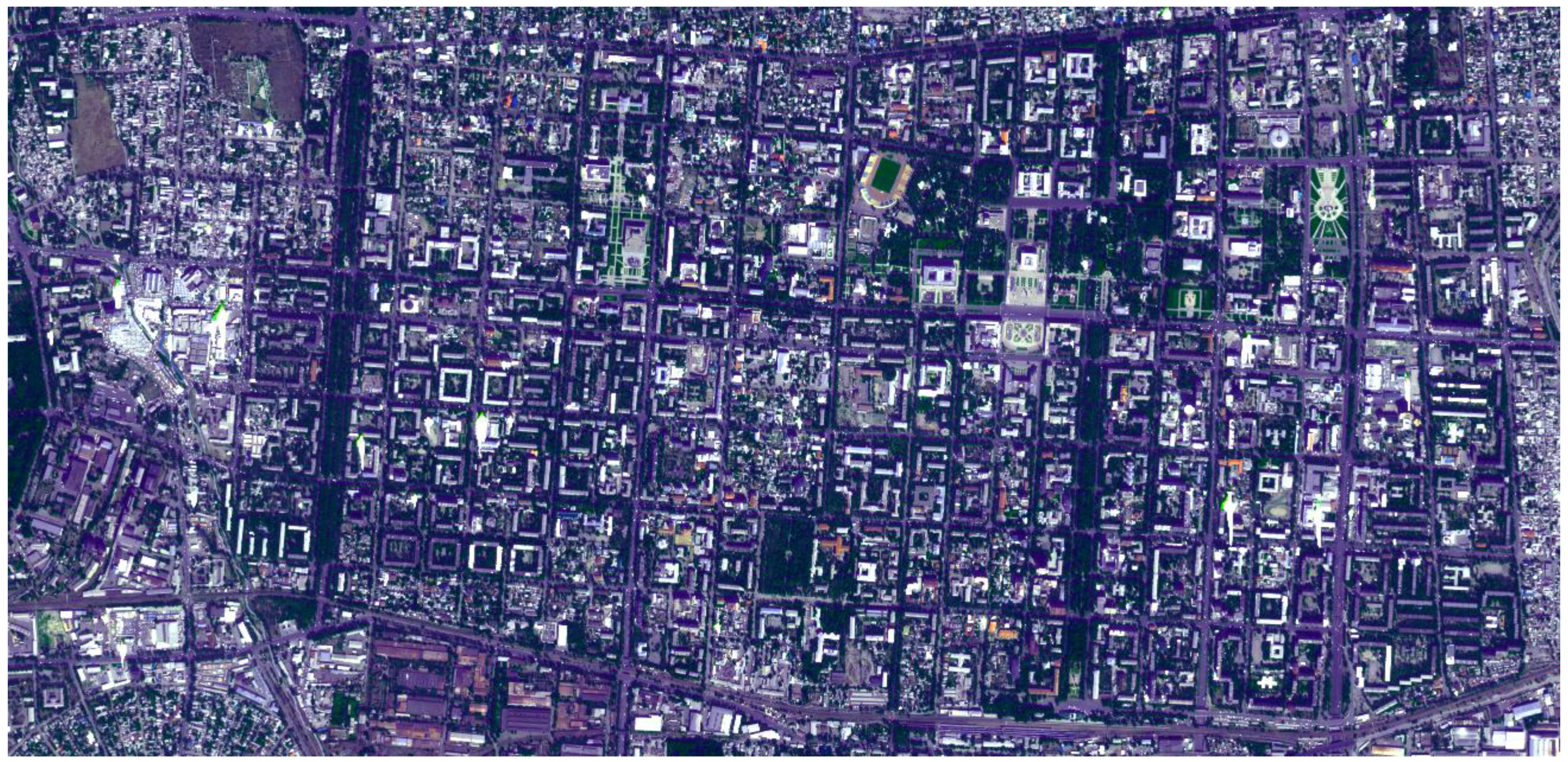
3. Detecting Urban Green Spaces from GeoEye-1 Data
3.1. Pre-Processing

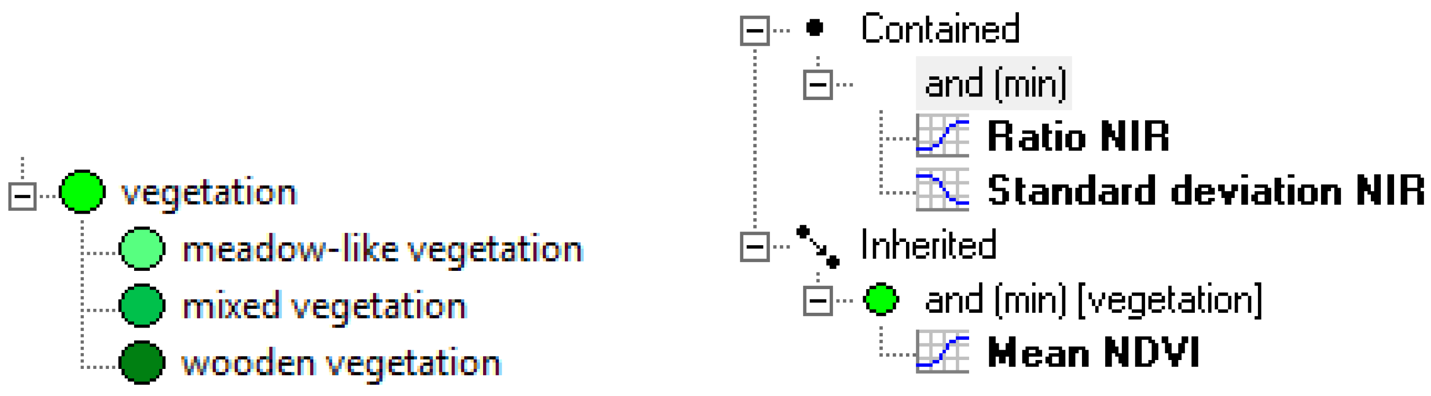
3.2. Object Based Image Analysis


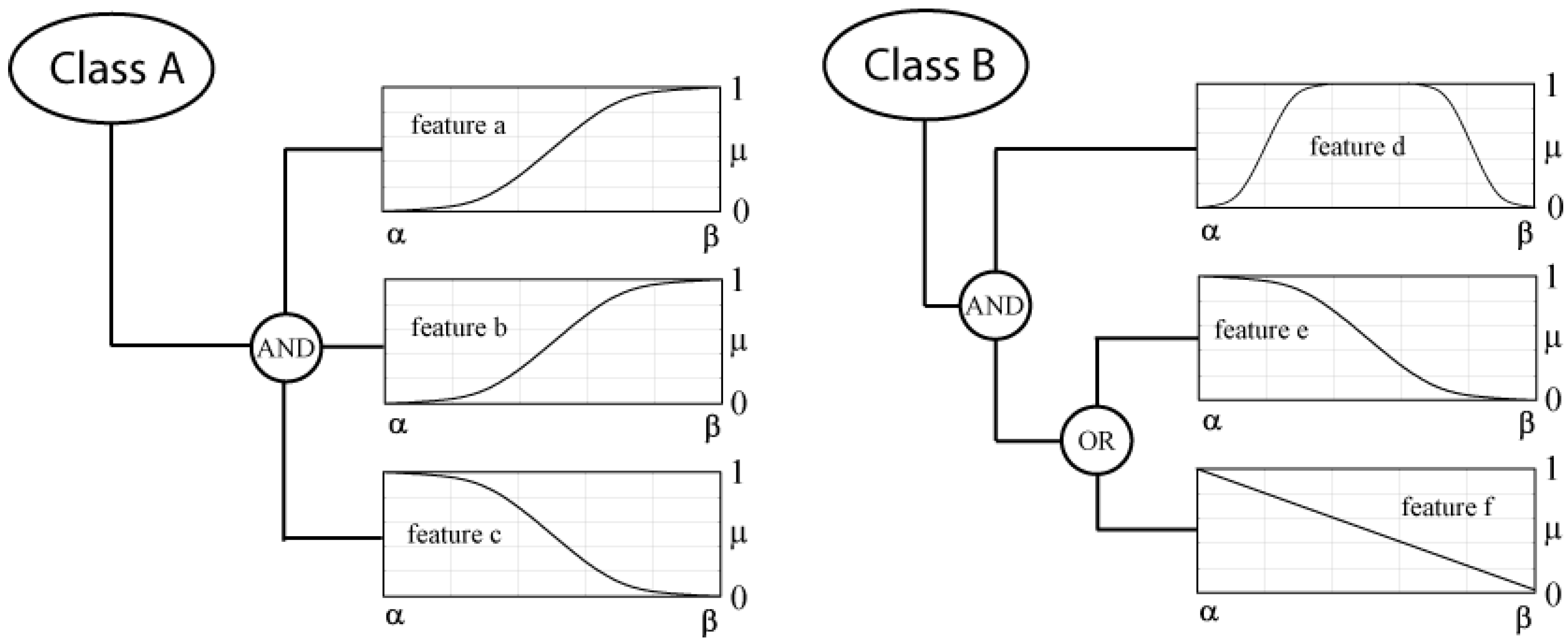
- object i is the more a member of class A, the closer its value of feature a and b is to β and the closer its value for feature c is to α.
- the final degree of membership to class A is the minimum membership value of the membership functions for feature a, b and c:
- the lower the value of feature f or e for object i is and the closer its value of feature d lies in the range between α and β, the more object i belongs to class B:

| Class | Property | Membership Function | Parameters of Membership Function | |
|---|---|---|---|---|
| α | β | |||
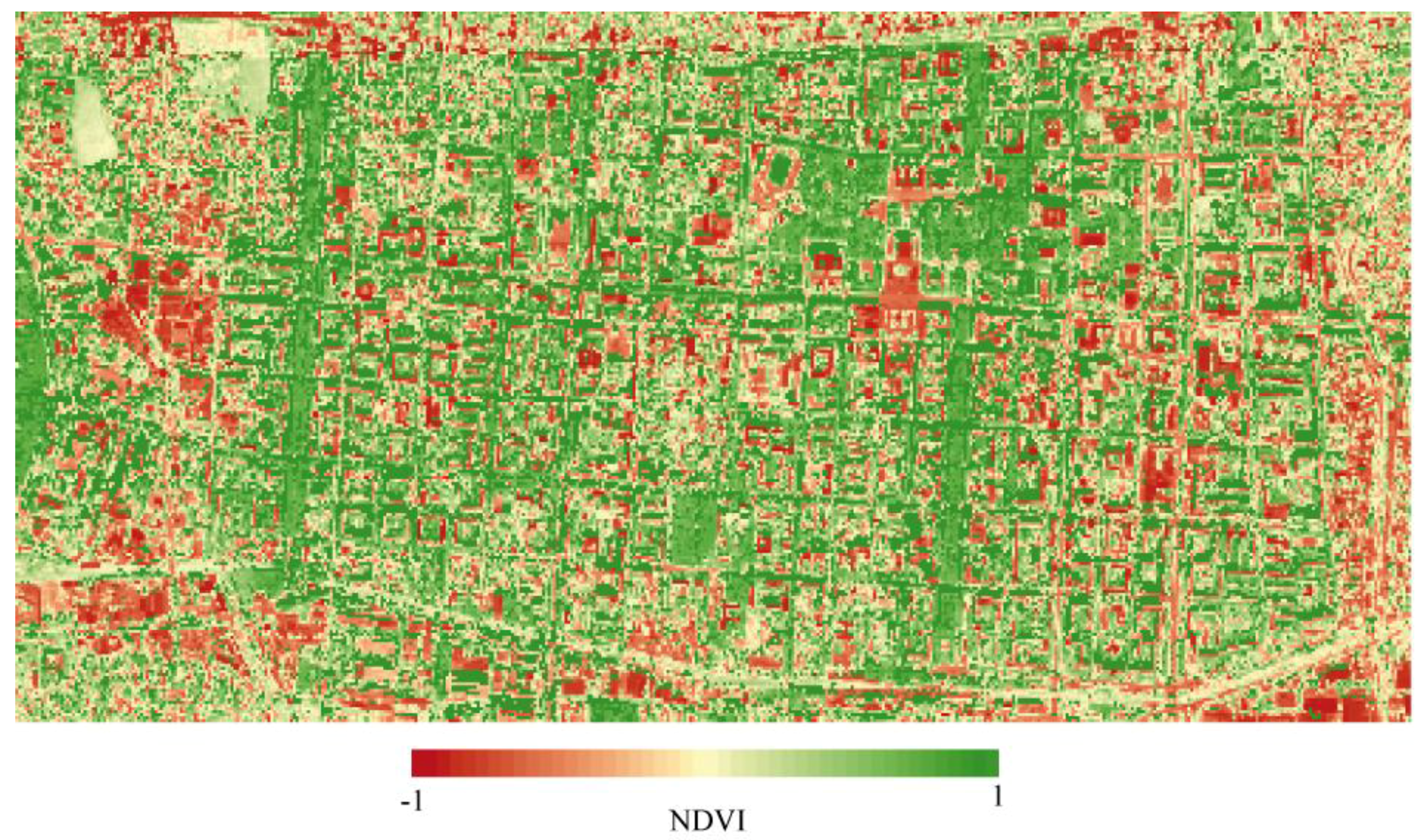
| vegetation | Mean NDVI |  | 0.45 | 0.60 |
| wooded vegetation | Ratio NIR |  | 0.40 | 0.50 |
| Standard Dev. NIR |  | 35.00 | 50.00 | |
| meadow-like vegetation | Ratio NIR |  | 0.40 | 0.70 |
| Standard Dev. NIR |  | 45.00 | 65.00 | |
| mixed vegetation | Ratio NIR |  | 0.45 | 0.75 |
| Standard Dev. NIR |  | 30.00 | 50.00 | |

| Class | No. of Objects | Mean | Standard Deviation | Min. | Max. |
| vegetation | 18,748 | 0.87 | 0.26 | 0.10 | 1.00 |
| After classifying vegetation child classes | |||||
| Class | No. of Objects | Mean | Standard Deviation | Min. | Max. |
| wooded vegetation | 9,232 | 0.65 | 0.30 | 0.10 | 1.00 |
| meadow-like vegetation | 644 | 0.84 | 0.22 | 0.10 | 1.00 |
| mixed vegetation | 8,003 | 0.86 | 0.21 | 0.11 | 0.99 |
| Class | No. of Objects | Mean | Standard Deviation | Min. | Max. |
| vegetation | 18,748 | 0.87 | 0.26 | 0.10 | 1.00 |
| After classifying vegetation child classes | |||||
| Class | No. of Objects | Mean | Standard Deviation | Min. | Max. |
| wooded vegetation | 9,232 | 0.64 | 0.32 | 0.00 | 1.00 |
| meadow-like vegetation | 644 | 0.47 | 0.35 | 0.00 | 1.00 |
| mixed vegetation | 8,003 | 0.72 | 0.30 | 0.00 | 1.00 |

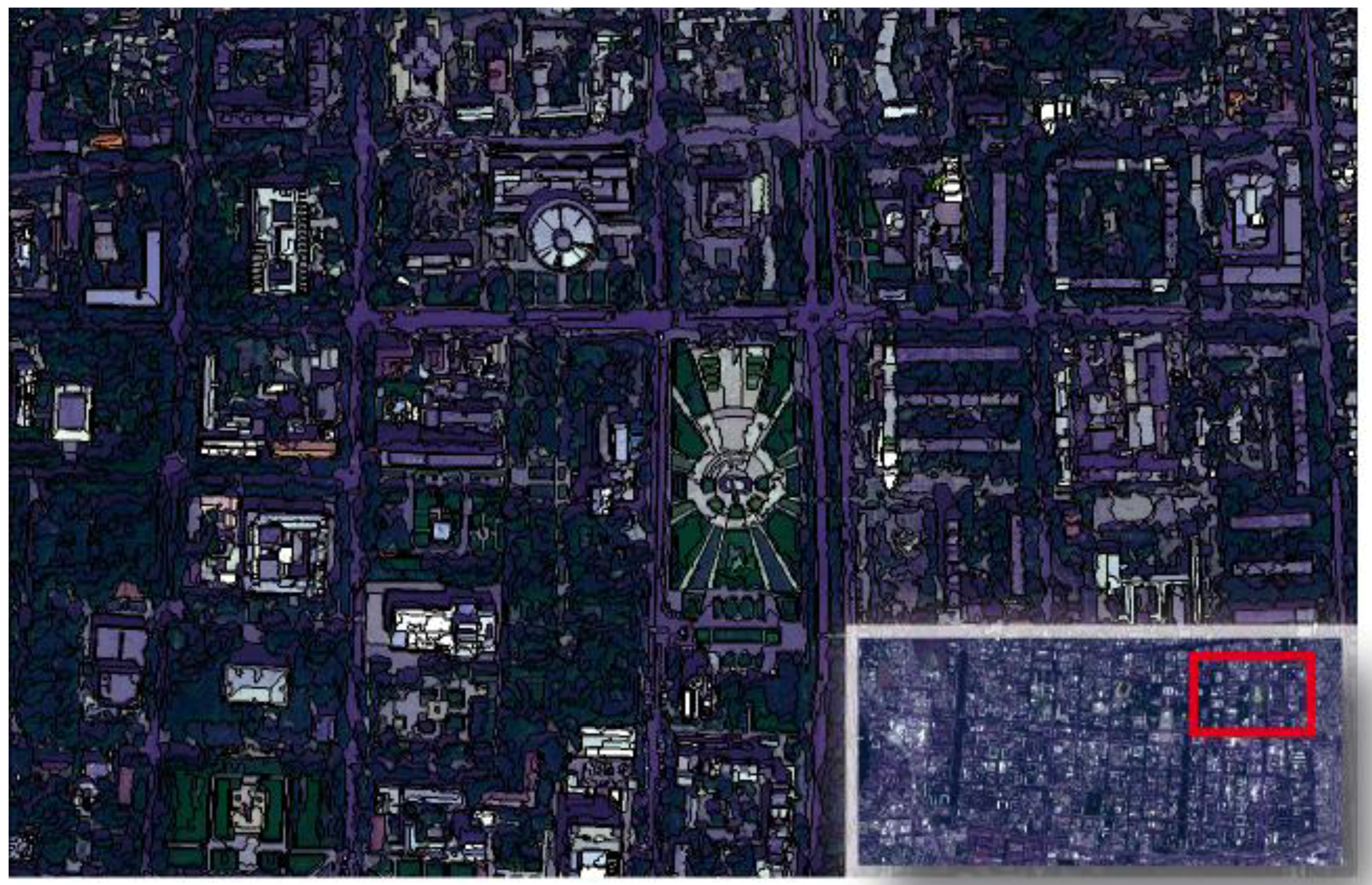
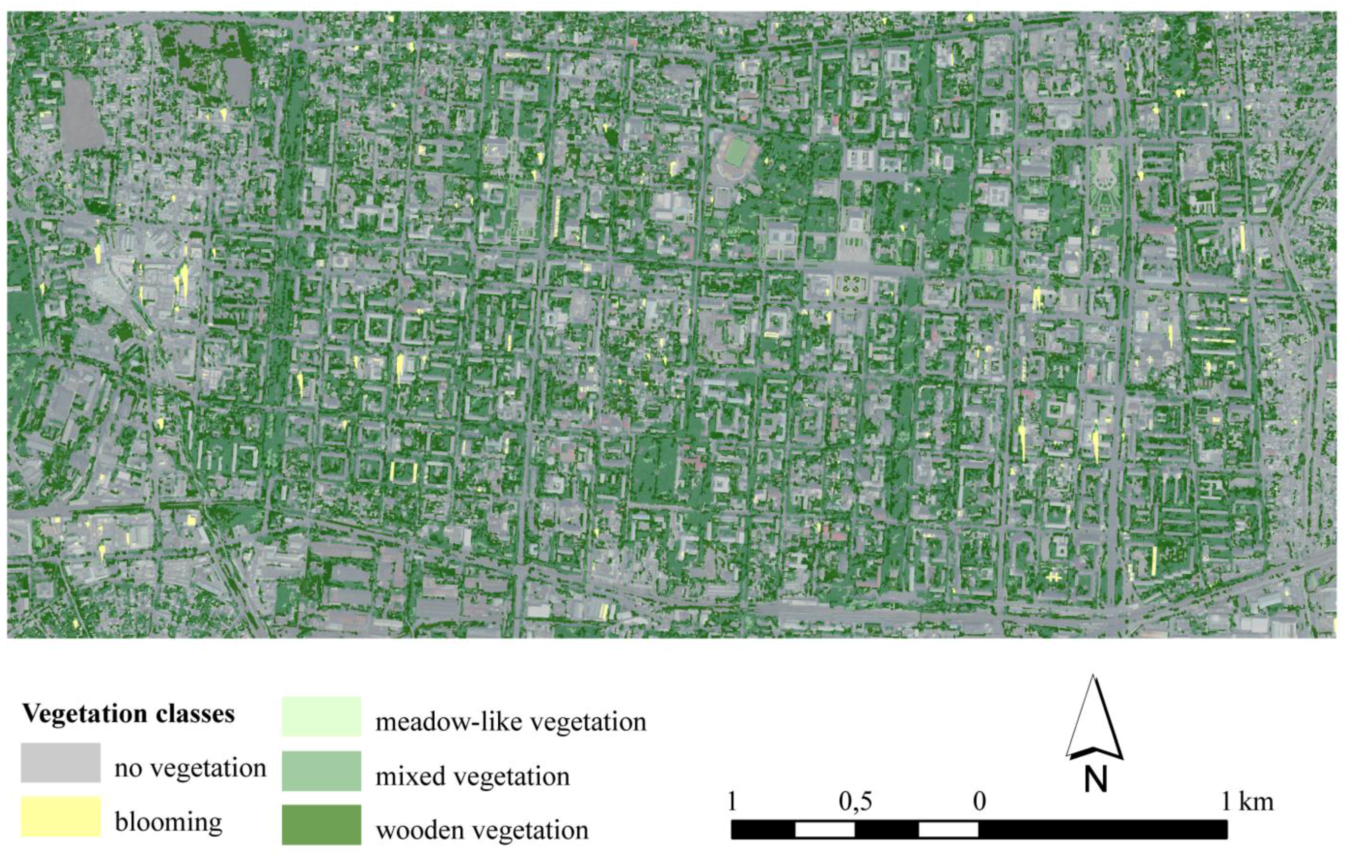
4. Spatial Analysis and Mapping
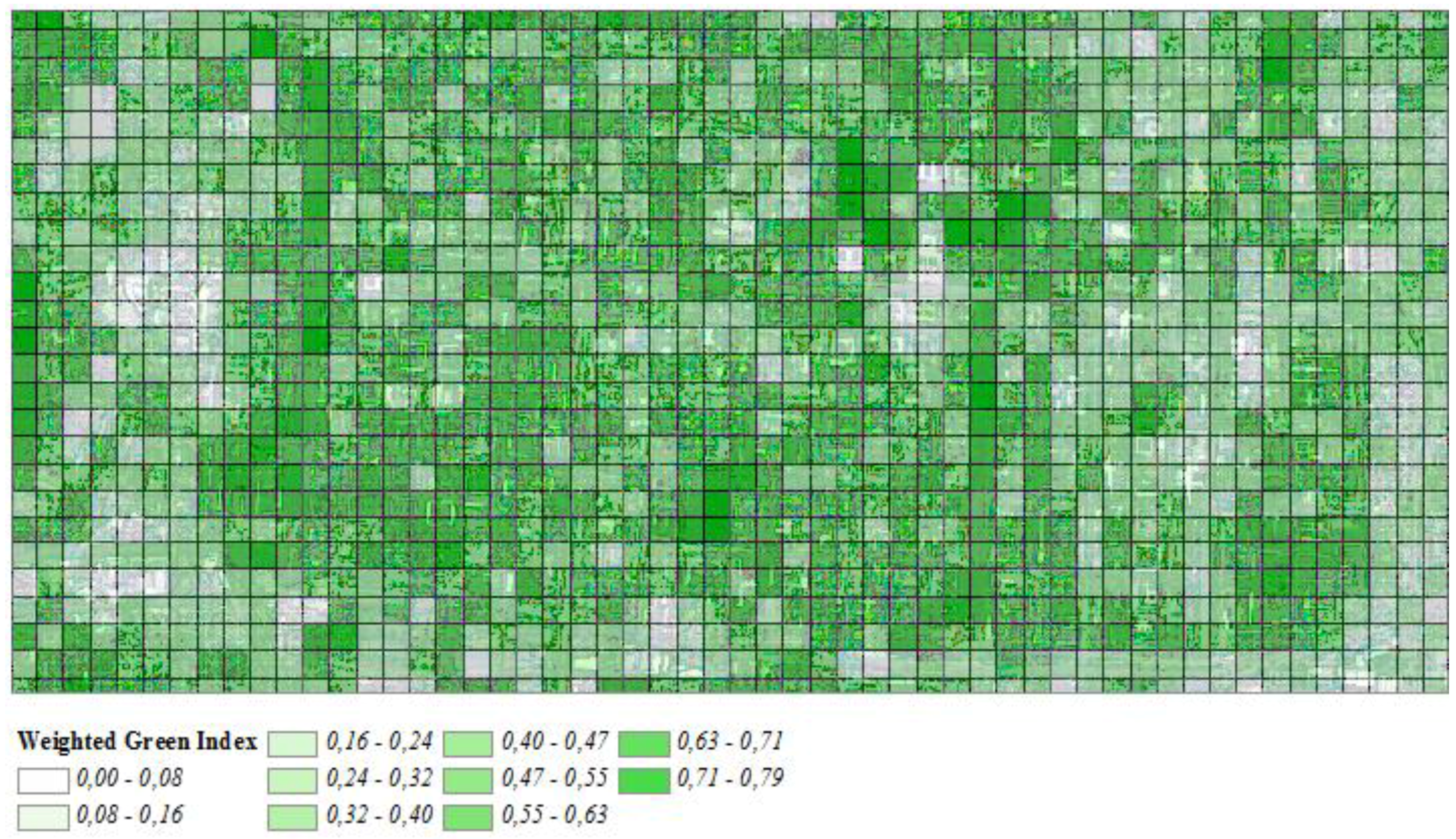
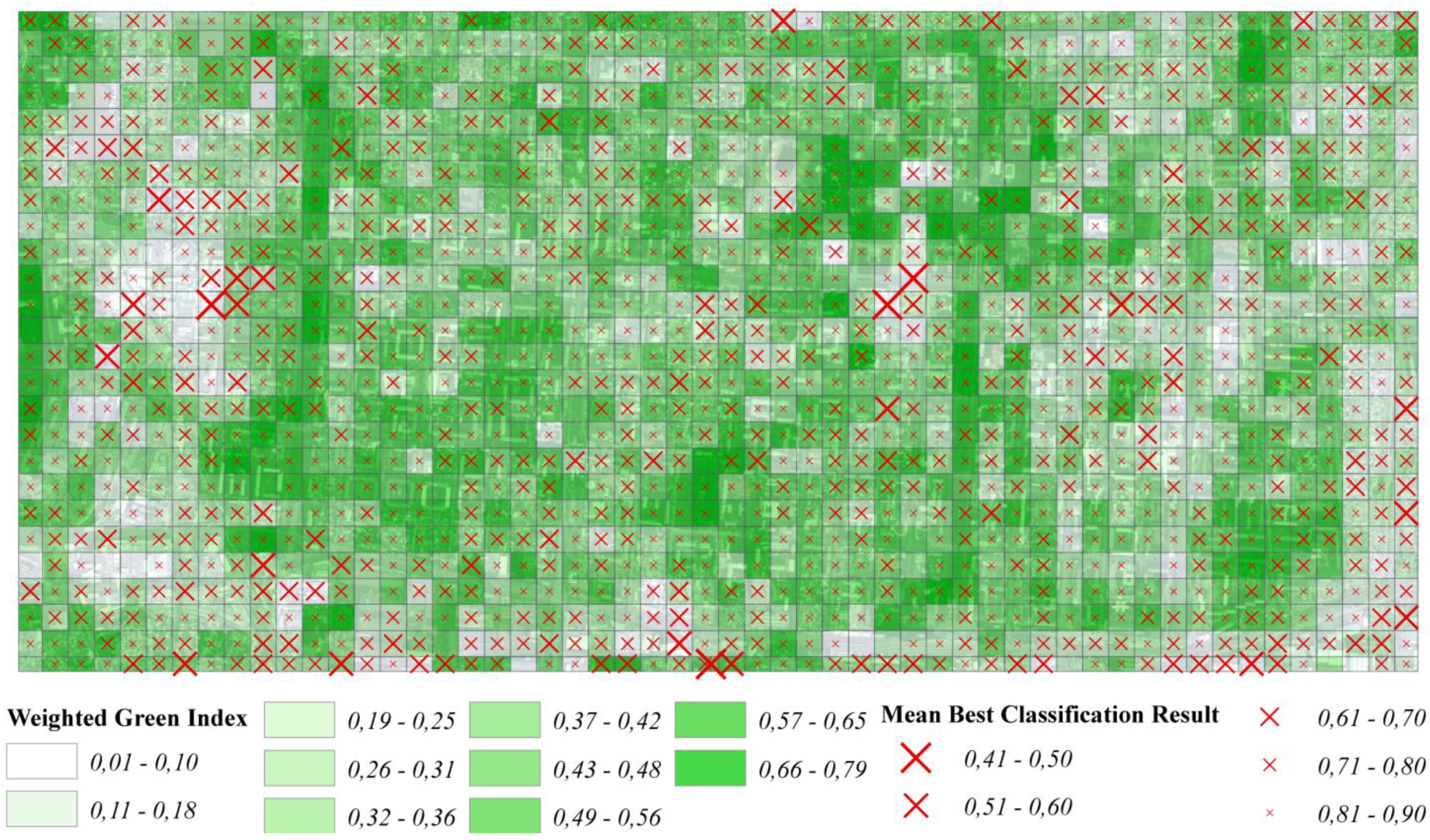
5. Developing an Urban Green Index
| Vegetation type | Weight |
|---|---|
| meadow-like vegetation | 0.3 |
| mixed vegetation | 0.8 |
| wooded vegetation | 1.0 |
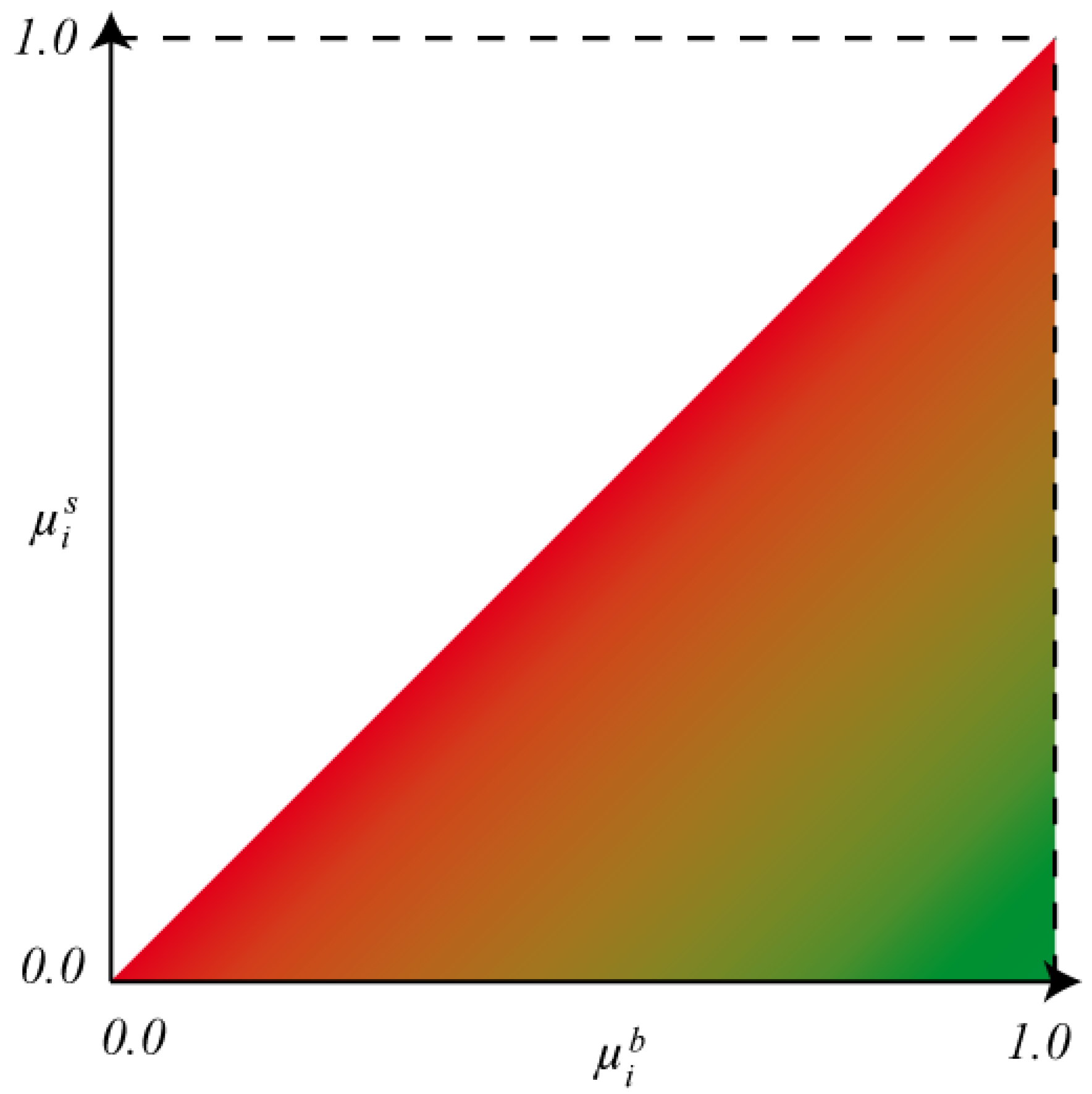
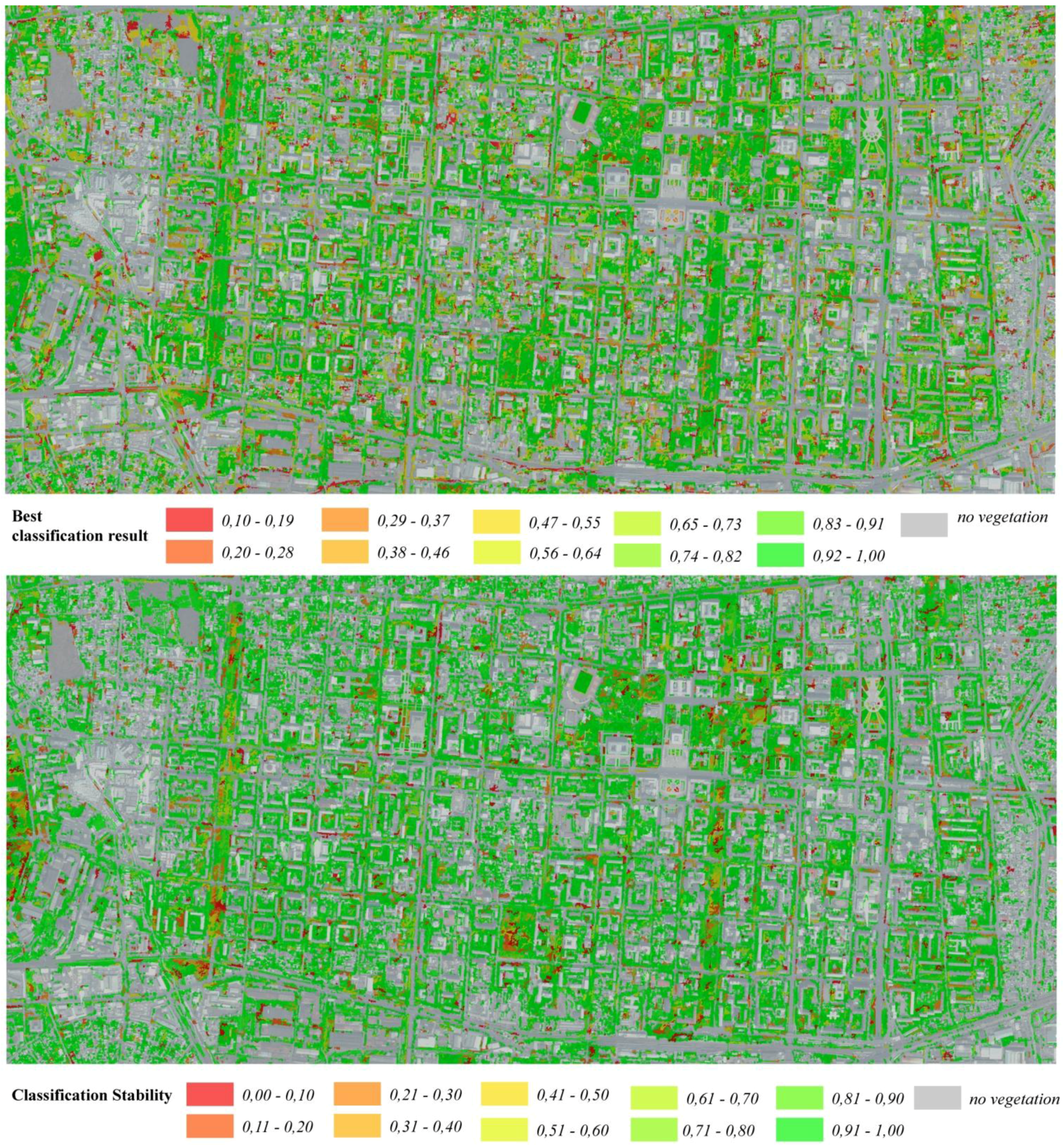
6. Impact of Classification Reliability on Analysis Results

7. Results and Discussion
Acknowledgments
References
- Zoulia, D.; Santamouris, M.; Dimoudi, A. Monitoring the effect of urban green areas on the heat island in Athens. Environ. Monit. Assess. 2009, 156, 275–292. [Google Scholar] [CrossRef] [PubMed]
- Alexandri, E.; Jones, P. Temperature decreases in an urban canyon due to green walls and green roofs in diverse climates. Build. Environ. 2008, 42, 480–493. [Google Scholar] [CrossRef]
- Robitu, M.; Musy, M.; Inard, C.; Groleau, D. Modeling the influence of vegetation and water pond on urban microclimate. Solar Energy 2006, 80, 435–447. [Google Scholar] [CrossRef]
- Schöpfer, E.; Lang, S.; Blaschke, T. A “Green Index” Incorporating Remote Sensing and Citizen’s Perception of Green Space. In Proceedings of the ISPRS Joint Conference on 3rd International Symposium Remote Sensing and Data Fusion Over Urban Areas (URBAN 2005) and 5th International Symposium Remote Sensing of Urban Areas (URS 2005), Tempe, AZ, USA, 14–16 March 2005; Volume 37, Part 5/W1. pp. 1–6.
- Welch, R.; Ehlers, M. Merging multiresolution SPOT HRV and Landsat TM Data. Photogramm. Eng. Remote Sensing 1987, 53, 301–303. [Google Scholar]
- Lillesand, T.M.; Kiefer, R.W.; Chipman, J.W. Remote Sensing and Image Interpretation, 6th ed.; John Wiley & Sons: Hoboken, NJ, USA, 2008. [Google Scholar]
- Lang, S. Object-based image analysis for remote sensing applications: modelling reality—Dealing with complexity. In Object Based Image Analysis; Blaschke, T., Lang, S., Hay, G.J., Eds.; Springer: Heidelberg/Berlin, New York, 2008; pp. 1–25. [Google Scholar]
- Haralick, R.M.; Shapiro, L. Survey: Image segmentation techniques. Comput. Vis. Graph. Image Process. 1985, 29, 100–132. [Google Scholar] [CrossRef]
- Pal, N.R.; Pal, S.K. A review on image segmentation techniques. Patt. Recog. 1993, 26, 1277–1294. [Google Scholar] [CrossRef]
- Baatz, M.; Schäpe, A. Multiresolution segmentation: An optimization approach for high quality multi-scale image segmentation. In Angewandte Geographische Informations—Verarbeitung; Strobl, J., Blaschke, T., Griesebner, G., Eds.; Wichmann Verlag: Karlsruhe, Germany, 2000; Volume XII, pp. 12–23. [Google Scholar]
- Neubert, M.; Meinel, G. Evaluation of Segmentation Programs for High Resolution Remote Sensing Applications. In Proceedings of the Joint ISPRS/EARSeL Workshop “High Resolution Mapping from Space 2003”, Hannover, Germany, 6–8 October 2003.
- Hay, G.J.; Blaschke, T.; Marceau, D.J.; Bouchard, A. A comparison of three image-object methods for the multiscale analysis of landscape structure. ISPRS J. Photogramm. Remote Sens. 2003, 57, 327–345. [Google Scholar] [CrossRef]
- Neubert, M.; Herold, H.; Meinel, G. Assessing image segmentation quality—Concepts, methods and application. In Object Based Image Analysis; Blaschke, T., Lang, S., Hay, G.J., Eds.; Springer: Heidelberg/Berlin, Germany, 2008; pp. 760–784. [Google Scholar]
- Thiel, C.; Thiel, C.; Riedel, T.; Schmullius, C. Object-based classification of SAR data for the delineation of forest cover maps and the detection of deforestation—A viable procedure and its application in GSE forest monitoring. In Object Based Image Analysis; Blaschke, T., Lang, S., Hay, G.J., Eds.; Springer: Heidelberg/Berlin, Germany, 2008; pp. 327–343. [Google Scholar]
- Lang, S.; Blaschke, T. Hierarchical Object Representation—Comparative Multiscale Mapping of Anthropogenic and Natural Features. In Proceedings of ISPRS Workshop “Photogrammetric Image Analysis”, Munich, Germany, 17–19 September 2003; Volume 34, pp. 181–186.
- Hay, G.J.; Castilla, G.; Wulder, M.A.; Ruiz, J.R. An automated object-based approach for the multiscale image segmentation of forest scenes. Int. J. Appl. Earth Obs. Geoinf. 2005, 7, 339–359. [Google Scholar] [CrossRef]
- Koestler, A. The Ghost in the Machine; Random House: New York, NY, USA, 1967. [Google Scholar]
- Câmara, G.; Souza, R.C.M.; Freitas, U.M.; Garrido, J. SPRING: Integrating remote sensing and GIS by object-oriented data modelling. Comput. Graph. 1996, 20, 395–403. [Google Scholar] [CrossRef]
- Lang, S.; Blaschke, T. Bridging Remote Sensing and GIS—What are the Main Supporting Pillars? In Proceedings of 1st International Conference on Object-based Image Analysis (OBIA 2006), Salzburg, Austria, 4–5 July 2006.
- Benz, U.; Hofmann, P.; Willhauck, G.; Lingenfelder, I.; Heynen, M. Multi-resolution object-oriented fuzzy analysis of remote sensing data for GIS-ready information. ISPRS J. Photogramm. Remote Sens. 2004, 58, 239–258. [Google Scholar] [CrossRef]
- Liedtke, C.-E.; Bückner, J.; Grau, O.; Growe, S.; Tönjes, R. AIDA: A System for the Knowledge Based Interpretation of Remote Sensing Data. In Proceedings of the Third International Airborne Remote Sensing Conference and Exhibition, Copenhagen, Denmark, 7–10 July 1997.
- Siler, W.; Buckley, J.J. Fuzzy Expert Systems and Fuzzy Reasoning; John Wiley & Sons: Hoboken, NJ, USA, 2005. [Google Scholar]
- Richards, J.A.; Jia, X. Remote Sensing Digital Image Analysis, 4th ed.; Springer: Berlin/Heidelberg, Germany, 2006. [Google Scholar]
- Cristianini, N.; Shawe-Taylor, J. An Introduction to Support Vector Machines; Cambridge University Press: Cambridge, UK, 2000. [Google Scholar]
- Zell, A.; Mamier, G.; Vogt, M.; Mache, N.; Hübner, R.; Döring, S.; Herrmann, K.-U.; Soyez, T.; Schmalzl, M.; Sommer, T.; et al. SNNS Stuttgart Neural Network Simulator, User Manual. Version 4.2. Available online: http://www.ra.cs.uni-tuebingen.de/downloads/SNNS/SNNSv4.2.Manual.pdf (accessed on 15 May 2011).
- Trimble. eCognition Developer 8.64.0 User Guide; Trimble: Munich, Germany, 2010. [Google Scholar]
- Trimble. eCognition Developer 8.64.0 Reference Book; Trimble: Munich, Germany, 2010. [Google Scholar]
- MacEachren, A.M.; Robinson, A.; Hopper, S.; Gardner, S.; Murray, R.; Gahegan, M.; Hetzler, E. Visualizing geospatial information uncertainty: What we know and what we need to know. Cartogr. Geogr. Inform. Sci. 2005, 32, 139–160. [Google Scholar] [CrossRef]
© 2011 by the authors; licensee MDPI, Basel, Switzerland. This article is an open access article distributed under the terms and conditions of the Creative Commons Attribution license (http://creativecommons.org/licenses/by/3.0/).
Share and Cite
Hofmann, P.; Strobl, J.; Nazarkulova, A. Mapping Green Spaces in Bishkek—How Reliable can Spatial Analysis Be? Remote Sens. 2011, 3, 1088-1103. https://doi.org/10.3390/rs3061088
Hofmann P, Strobl J, Nazarkulova A. Mapping Green Spaces in Bishkek—How Reliable can Spatial Analysis Be? Remote Sensing. 2011; 3(6):1088-1103. https://doi.org/10.3390/rs3061088
Chicago/Turabian StyleHofmann, Peter, Josef Strobl, and Ainura Nazarkulova. 2011. "Mapping Green Spaces in Bishkek—How Reliable can Spatial Analysis Be?" Remote Sensing 3, no. 6: 1088-1103. https://doi.org/10.3390/rs3061088
APA StyleHofmann, P., Strobl, J., & Nazarkulova, A. (2011). Mapping Green Spaces in Bishkek—How Reliable can Spatial Analysis Be? Remote Sensing, 3(6), 1088-1103. https://doi.org/10.3390/rs3061088