Monitoring Urban Tree Cover Using Object-Based Image Analysis and Public Domain Remotely Sensed Data

Abstract

Urban forest ecosystems provide a range of social and ecological services, but due to the heterogeneity of these canopies their spatial extent is difficult to quantify and monitor. Traditional per-pixel classification methods have been used to map urban canopies, however, such techniques are not generally appropriate for assessing these highly variable landscapes. Landsat imagery has historically been used for per-pixel driven land use/land cover (LULC) classifications, but the spatial resolution limits our ability to map small urban features. In such cases, hyperspatial resolution imagery such as aerial or satellite imagery with a resolution of 1 meter or below is preferred. Object-based image analysis (OBIA) allows for use of additional variables such as texture, shape, context, and other cognitive information provided by the image analyst to segment and classify image features, and thus, improve classifications. As part of this research we created LULC classifications for a pilot study area in Seattle, WA, USA, using OBIA techniques and freely available public aerial photography. We analyzed the differences in accuracies which can be achieved with OBIA using multispectral and true-color imagery. We also compared our results to a satellite based OBIA LULC and discussed the implications of per-pixel driven vs. OBIA-driven field sampling campaigns. We demonstrated that the OBIA approach can generate good and repeatable LULC classifications suitable for tree cover assessment in urban areas. Another important finding is that spectral content appeared to be more important than spatial detail of hyperspatial data when it comes to an OBIA-driven LULC.

1. Introduction

Urban landscapes are a unique combination of natural and built environments. Natural systems and the intertwined ecological services they provide are key components of a city’s infrastructure. For example, a city’s urban tree cover could be considered part of the local storm water management system, aiding in pollutant filtration, and reduction of surface runoff and thermal loading on streams. However, our ability to quantify and monitor these services over time is heavily dependent on accurate and timely tree cover assessments, which can also be used to optimize ecosystem health and resiliency [1]. These assessments are typically achieved through field methods limited by access to private lands. Moreover, few cities have adequate staff or budget resources that are required to undertake urban forestry assessments to achieve planning and management goals. Remote sensing approaches can provide a complimentary, spatially explicit dataset that can be used to devise an on ground sampling regime. Moreover, remote sensing canopy assessments are reasonably simple and can be conducted quickly, inexpensively, and without access or disturbance issues encountered in ground-based data collections [2,3]; thus, they can provide valuable supplemental information in areas that cannot be accessed on the ground. These spatially explicit assessments provide a means to measure and monitor over time complex urban environments, and their dynamic ecologies [4,5], for example, through the use of spatial metrics [6]. For instance, tree cover surveys and forest pattern metrics are useful to help a city quantify current tree cover status [7], determine the locations and drivers of cover loss or gain [8], and monitor these trends over time [9]. These data can then be used to establish tree protection requirements for new developments, assist with urban tree health management, and determine target areas for planting projects. Tree cover information is but one variable available from this remote sensing approach, which can also provide information on impervious surfaces and many other ground covers.

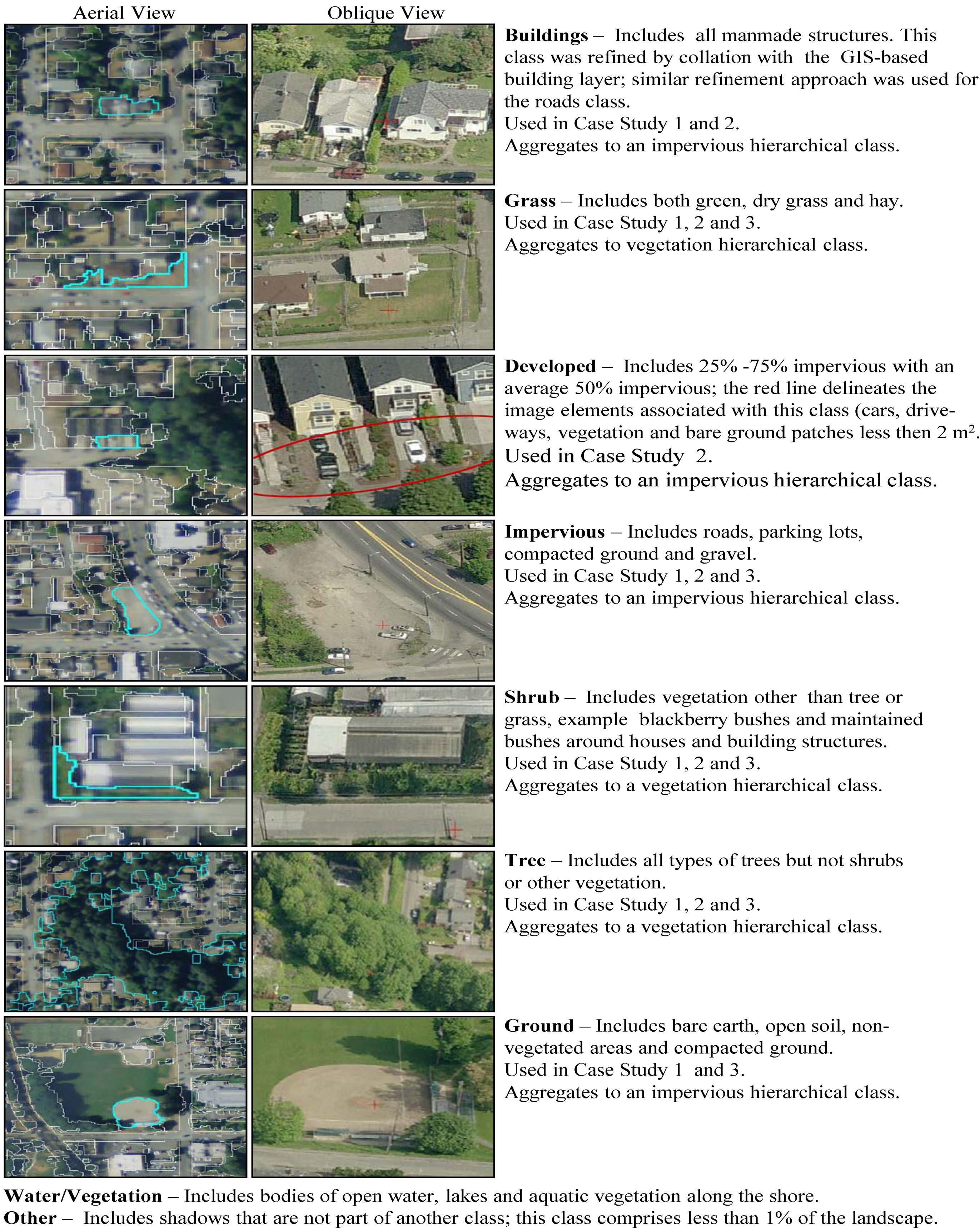
Land use/land cover (LULC) classifications are often created to visually assess the composition of urban landscapes and quantify different aspects of the environment. “Land cover” describes natural and built objects covering the land surface, while “land use” documents human uses of the landscape [10]. Remote sensing imagery effectively captures characteristics of the Earth’s surface, but it takes an interpreter’s knowledge about shape, texture, patterns, and site context to derive information about land use activities from information about land cover [11]. Classifications typically utilize some modification of the Anderson hierarchical system (Table 1), with generalized LULC classes described at Levels I and II and more detailed classifications for Levels III and beyond [10]. Land use/land cover needs to be classified at a very fine scale to be effective for city planning and urban land management [11,12,13].

Table 1. Anderson hierarchical classification system showing examples of Levels I–III for Urban and Forest Lands [10]; only the classes in red and green have been expanded upon in the hierarchies.

Level I	Level II	Level III
$\text{1. Urban/Build-up Land}$	$\text{11. Residential}$	111. Single-family Units
	12. Commercial and Services	112. Multiple-family Units
	13. Industrial	113. Group Quarters
	14. Transportation, Communications and Utilities	114. Residential Hotels
	15. Industrial and Commercial Complexes	115. Mobile Home Parks
	16. Mixed Urban or Built-up Land	116. Transient Lodging
	17. Other Urban or Built-up Land	117. Other
….
$\text{4. Forested Land}$	41. Deciduous Forest Land	421. Natural/Unmanaged Trees
	$\text{42. Evergreen Forest Land}$	422. Natural/Managed Park Trees
	43. Mixed Forest Land	423. Managed Residential/Street Trees
		423. Plantation Trees

Table 1. Anderson hierarchical classification system showing examples of Levels I–III for Urban and Forest Lands [10]; only the classes in red and green have been expanded upon in the hierarchies.

Level I	Level II	Level III
$\text{1. Urban/Build-up Land}$	$\text{11. Residential}$	111. Single-family Units
	12. Commercial and Services	112. Multiple-family Units
	13. Industrial	113. Group Quarters
	14. Transportation, Communications and Utilities	114. Residential Hotels
	15. Industrial and Commercial Complexes	115. Mobile Home Parks
	16. Mixed Urban or Built-up Land	116. Transient Lodging
	17. Other Urban or Built-up Land	117. Other
….
$\text{4. Forested Land}$	41. Deciduous Forest Land	421. Natural/Unmanaged Trees
	$\text{42. Evergreen Forest Land}$	422. Natural/Managed Park Trees
	43. Mixed Forest Land	423. Managed Residential/Street Trees
		423. Plantation Trees

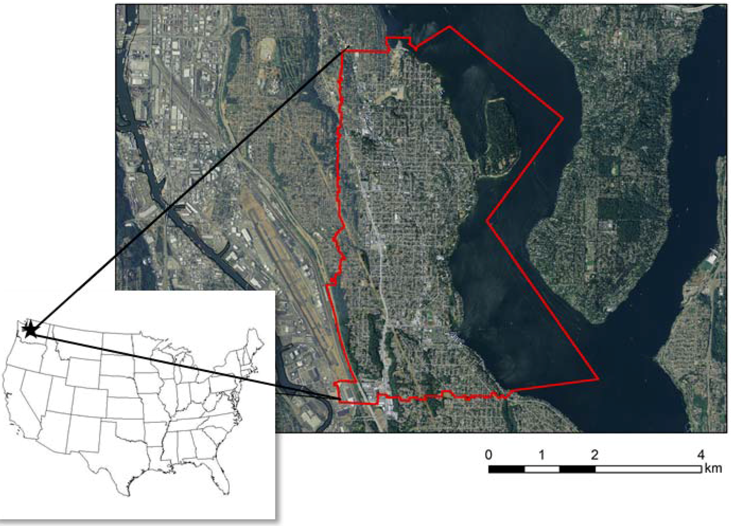
In 2006, City of Seattle launched the Environmental Action Agenda, which called for an increase in urban tree cover from the existing 18% to 30% in 30 years [14]; this assessment was performed by non-spatially explicit, semi-manual image interpretation [15]. This ambitious policy goal would attain the difference in current estimated and planned urban forest cover and certainly increase the urban forest. To establish a spatially explicit baseline, an independent remotely sensed-based urban tree cover assessment was contracted in 2007 by the City of Seattle. Native Communities Development Corporation (NCDC) used high spatial resolution or hyperspatial [16] QuickBird satellite imagery in this assessment and tree cover was reported at 22.9% [15]. If an overall goal for tree cover is 30%, as is common for many Pacific Northwest cities, a 5% discrepancy in cover could affect planning, management, and policy decisions aimed at increasing overall urban tree cover. As such, a good monitoring program is required not only in Seattle, but most urban areas interested in preserving or increasing their tree cover. An effective monitoring program will help us quantify how much tree cover there was in the past, is currently, and will be in the future in order to meet tree cover goals.

Remote sensing technologies can provide a means to classify tree cover and a variety of other continuous environmental variables over large spatial extents and moderate temporal extents [9]. Interestingly, remote sensing of urban forests originally evolved from aerial photography assessment to coarse pixel remote sensing and now is returning to hyperspatial image analysis [17]. Traditional pixel-based classification methods use Landsat satellite imagery to produce LULC maps (e.g., 2001 National Land Cover Database) by assigning individual pixels to a specific class based on a unique spectral signature [11,18]. These coarse per-pixel resolution data, including Landsat, AVHRR and MODIS, generally have greater spectral extents (Landsat) and temporal extents (AVHRR and MODIS), compared to hyperspatial satellite (e.g., QuickBird and IKONOS) and aerial photography (e.g., US National Agricultural Imagery Program—NAIP). Thus, moderate resolution remote sensing has played a critical role in urban tree cover assessment at regional and global scales [19,20]. However, in general, the spatial resolution of Landsat imagery (30 m) limits the ability to identify and map features within a property parcel, yet, decision making typically takes place at the parcel level, and 900 m² is larger than most urban property parcels [13]. Furthermore, in heterogeneous canopies found in urban environments, the scale between what is considered a forest patch and what can be resolved by a 30 m or coarser pixel presents a special challenge [17]. Thus, it is now a well-accepted principle that this moderate resolution imagery is not appropriate for LULC mapping in heterogeneous urban areas [12,13,18].

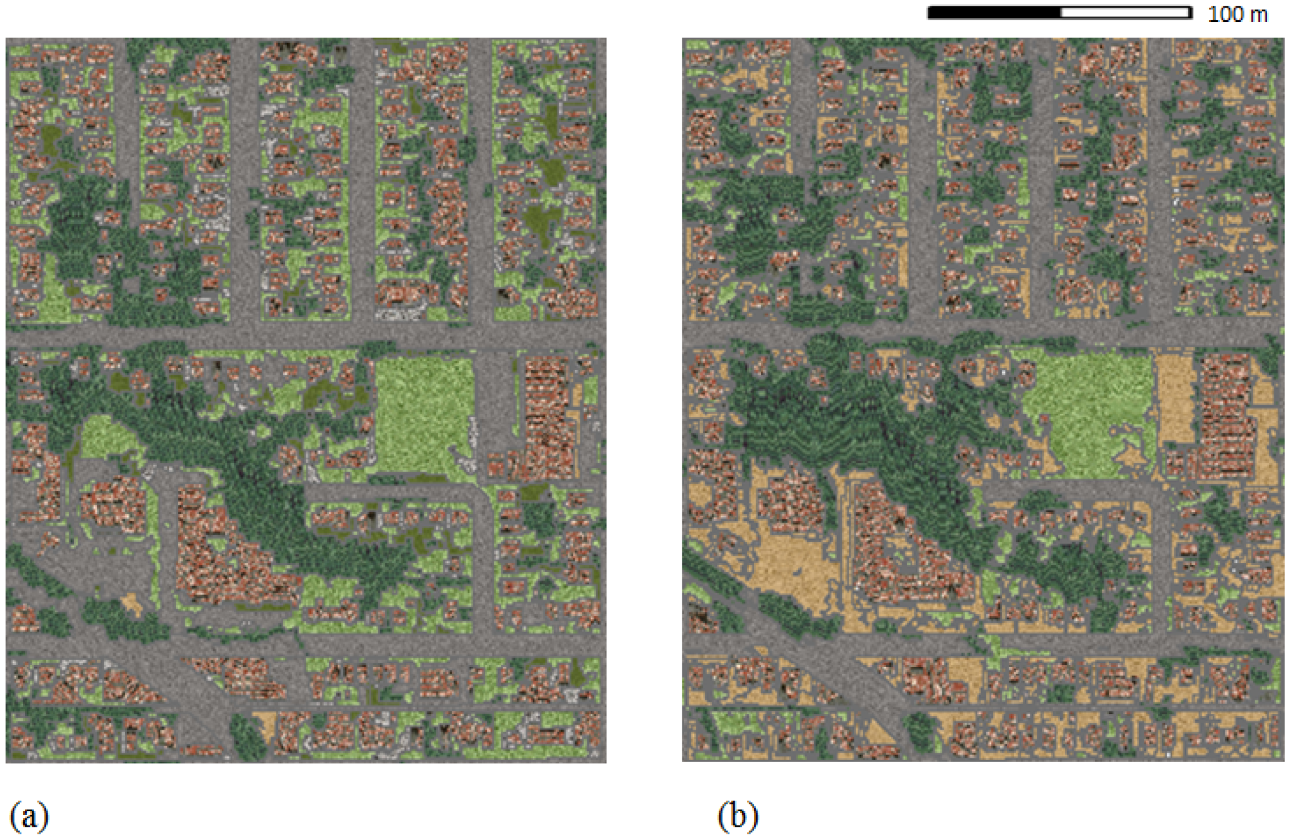
A relatively new classification method, object-based image analysis (OBIA), sometimes referred to as feature extraction, feature analysis or object-based remote sensing, appears to work best on hyperspatial satellite and aerial imagery as well as LiDAR [11,13]. This form of feature extraction allows for use of additional variables such as shape, texture, and contextual relationships to classify image features. This can both improve accuracy results and allows us to map very small urban features, such as mature individual trees or small clusters of shrubs [21,22]. Furthermore, others have shown that per-pixel classification approaches, although appropriate on Landsat imagery, are outperformed by OBIA approaches on hyperspatial imagery in urban, suburban, and agricultural landscapes [21] and in the urban-wildland interface, especially in instances where the tree cover is complex and heterogeneous [18]. The significant strength of OBIA is that it can also be used on free, publicly available, hyperspatial, NAIP imagery, which is limited in the number of spectral bands available. NAIP imagery has a national extent, offers repeatability, allows for spatial and often spectral comparability, and can be classified to achieve detailed LULC maps for urban planning, management, and scientific research [13,21]. OBIA approach on NAIP imagery has been used in other applications, specifically wetland detection [23], but its utility in urban tree cover mapping has not been explored.

The purpose of this study was to examine the ability of OBIA methods using freely-available, public domain imagery and ancillary datasets for classifying land use and land cover in a heterogeneous urban landscape with suitable detail to allow for monitoring and planning at the parcel level. Therefore, specific attention is paid to developing a method that not only determines the amount or extent of tree cover, but also provides the explicit spatial location of that tree cover. It was our goal to generate a repeatable algorithm that can be tailored for use with imagery that might have other spatial/spectral resolutions and that could allow for the integration of other data sources.

Specific objectives included:

(1)

create a flexible algorithm,

(2)

test algorithm performance on imagery of varying spatial and spectral resolutions, and

(3)

assess the accuracy and implications for tree cover assessment of the resulting classifications, specifically, the implication on ground sampling design.

We aimed to develop an accurate method that is repeatable on future dates of imagery and at other locations.

2. Methods

2.1. Study Area

We created an OBIA algorithm for a small, yet diverse pilot study area in Seattle, WA, USA. Seattle is unique in that it has a diverse evergreen and deciduous tree cover due to distinct soils and microclimates resulting from glacially-carved topography and human activity. The pilot study area (hereafter referred to as ‘Rainier Valley’) is the ‘98118’ zip code, which covers approximately 1,585 ha of the southeastern portion of the Seattle, and extends between Latitude: 47°34″20′ and 47°30″36′N and Longitude: 122°17″39′ and 122°14″46′W (Figure 1). The area is situated within the Puget Sound region of Western Washington with elevations ranging from approximately 0 to 106 m above mean sea level, and contains urban land uses, including single- and multi-family residential, commercial/mixed use, industrial, institutional, developed parks, and natural areas. A majority of land in the region was forested prior to the settlement of present-day Seattle during the mid-nineteenth century. Seward Park has about 49 ha of remnant of old growth forest, and provides a glimpse of what much of the area used to look like. We selected this zip code for our pilot study area because it is said to be the most culturally diverse in the US [24,25] and has several socioeconomic characteristics such as a wide divergence in education, which could affect urban tree cover [26]. Due to this diversity, the variety of LULC in this zip code encompasses the range we expect to see in the whole of the Seattle area.

Figure 1. Map of study area showing Rainier Valley zipcode boundary.

Figure 1. Map of study area showing Rainier Valley zipcode boundary.

2.2. Datasets

We used two types of remotely sensed data for the OBIA classifications presented in this research and compared our work to a third independent tree cover assessment project created for the City of Seattle using the OBIA technique [15]. Finally, we also used the 2001 National Land Cover Database (NLCD), a nationwide moderate resolution (30 m) % canopy cover product derived from per-pixel driven classifiers using Landsat satellite and generated by the US Geological Survey (USGS) [27]; the 2006 data were not available at the time of analysis.

We chose a public domain, 2009 dataset consisting of orthorectified TIFF imagery acquired during leaf-on summer months (August) with four spectral bands including three color and one near-infrared bands; allowing for false-color imagery display. The NAIP imagery was acquired with the Leica ADS80 Digital Imaging Sensor, at a one-meter ground sample distance (GSD) with a horizontal accuracy that matched within six meters of photo-identifiable ground control points, which were used during image inspection. The reference system used was NAD 1983/UTM Zone 10N. We selected these images because the spectral and spatial resolutions should be sufficient to capture small urban features in order to produce a detailed classification and because the imagery was readily available at no cost. We also acquired a 2002 NAIP imagery which consisted of orthorectified TIFF imagery collected during the leaf-on month of June with three spectral bands in the color range (true-color) of the electromagnetic spectrum; no near-infrared band was acquired with the film based sensor. The imagery GSD was 30 cm with horizontal accuracies similar to NAIP imagery; these data were also furnished freely by the USGS.

We were also given access to 2009 true-color oblique photography of our study area collected by King County, Washington State. The data were accessible through Pictometry extensions for ArcGIS and used for the visual classification accuracy assessment. In addition to the oblique view, four-direction neighborhood-level views were available, at a nominal ground sample distance (GSD) of 15 cm. We also applied these data in the visual classification accuracy assessment.

For comparative purposes only, we used a 2007 QuickBird-based NCDC LULC classification, which was created using the OBIA technique with the goal of determining existing urban tree cover and potential tree planting sites [16] in the city of Seattle, WA, USA.

The City of Seattle put a lot of prior investment into producing parcel datasets, building footprints, road layers, etc. These datasets were also utilized because they are a good publically available free resource which can be downloaded online from the City of Seattle website, and can save time necessary for classification development and/or refinement. All datasets, dates, sources, description and uses in our project are summarized in Table 2.

2.3. Land Use/Land Cover Classifications

We developed LULC classifications using two temporally spaced datasets with varying spatial and spectral resolution. We used Definiens 8.0 to create classification algorithms individualized for each date of imagery. Although the two classification algorithms follow a similar basic structure, the features used to create the algorithms are quite different from one another. This is due to spatial and spectral resolution of each set of imagery as well as the timing of image acquisition. Further, we used the same ancillary data for both algorithms: a King County parcel shapefile and a building footprint shapefile. The building footprint shapefile was created in 1993 and did not perfectly represent the building outlines, but it was valuable as a tool to locate buildings that could later be grown or subtracted from based on segments generated from the imagery.

Table 2. Summary of datasets.

Dataset	Date	Source	Description	Used For
GIS Roads Shapefile	2006	City of Seattle	Manually derived road centerlines	Primary Segmentation; Visual Assessment of Classification Accuracy
GIS Building Footprints Shapefile	1993	City of Seattle	Manually derived building footprints	Primary Segmentation; Visual Assessment of Classification Accuracy
NAIP 2002	Jun-02	NAIP	Aerial ortho-rectified photography (3-band true color); 30 cm GSD	Primary Segmentation; Secondary Segmentation, Classification; Visual Assessment and Class Refinement
NAIP 2009	Aug-09	NAIP	Aerial ortho-rectified photography (4-band infrared); 1 m per pixel resolution	Primary Segmentation; Secondary Segmentation, Classification; Visual Assessment and Class Refinement
QuickBird	Jun-07	City of Seattle	4-band infrared imagery; 0.6 m per pixel resolution	NCDC OBIA Based Methods [ 16]
NLCD % Canopy Cover	2001	USDA	2001 per-pixel classification derived dataset	Generating Field Sampling Points
Homogeneity Texture 2002	2009	2009 NAIP	derived from red back of the NAIP 2002 imagery, using all adjacent pixels, 0.3 per pixel resolution	Classification Algorithm
Homogeneity Texture 2009	2002	2002 NAIP	derived from red back of the NAIP 2002 imagery, using all adjacent pixels, 0.3 per pixel resolution	Classification Algorithm
2009 oblique photography	Jun-09	King County GIS	true color, four-direction neighborhood-level views were available, at a nominal ground sample distance (GSD) of 15 cm	Visual Assessment and Decision Making for Class Refinement

Table 2. Summary of datasets.

Dataset	Date	Source	Description	Used For
GIS Roads Shapefile	2006	City of Seattle	Manually derived road centerlines	Primary Segmentation; Visual Assessment of Classification Accuracy
GIS Building Footprints Shapefile	1993	City of Seattle	Manually derived building footprints	Primary Segmentation; Visual Assessment of Classification Accuracy
NAIP 2002	Jun-02	NAIP	Aerial ortho-rectified photography (3-band true color); 30 cm GSD	Primary Segmentation; Secondary Segmentation, Classification; Visual Assessment and Class Refinement
NAIP 2009	Aug-09	NAIP	Aerial ortho-rectified photography (4-band infrared); 1 m per pixel resolution	Primary Segmentation; Secondary Segmentation, Classification; Visual Assessment and Class Refinement
QuickBird	Jun-07	City of Seattle	4-band infrared imagery; 0.6 m per pixel resolution	NCDC OBIA Based Methods [ 16]
NLCD % Canopy Cover	2001	USDA	2001 per-pixel classification derived dataset	Generating Field Sampling Points
Homogeneity Texture 2002	2009	2009 NAIP	derived from red back of the NAIP 2002 imagery, using all adjacent pixels, 0.3 per pixel resolution	Classification Algorithm
Homogeneity Texture 2009	2002	2002 NAIP	derived from red back of the NAIP 2002 imagery, using all adjacent pixels, 0.3 per pixel resolution	Classification Algorithm
2009 oblique photography	Jun-09	King County GIS	true color, four-direction neighborhood-level views were available, at a nominal ground sample distance (GSD) of 15 cm	Visual Assessment and Decision Making for Class Refinement

The general steps in our methods included: (1) a primary segmentation using imagery and ancillary building and roads layers to separate vegetation and impervious cover; (2) a secondary segmentation within each of the primary classes using various derivatives (e.g., texture) and spatial and spectral characteristics of the imagery; and (3) a classification using features derived from the imagery. Although the algorithms are too lengthy to describe in their entirety, there are specific themes that were useful in their creation, and are described in more detail below. The target classes used in our approach and in the 2007 dataset created by NCDC are shown and described in Figure 2. Our aim was to produce classes that could be hierarchically aggregated back to the vegetation and impervious covers, suitable for future ecological modeling and applications.

Figure 2. Example of image segments representative of the described LULC classes. Cyan polygons show an example of the LULC class being delineated in the OBIA segmentation, adjacent segments are shown in white and can represent a different class. The oblique image is centered on the delineated segment. The 2002 aerial and co-registered 2009 oblique images are not shown at the same scale; north is up.

Figure 2. Example of image segments representative of the described LULC classes. Cyan polygons show an example of the LULC class being delineated in the OBIA segmentation, adjacent segments are shown in white and can represent a different class. The oblique image is centered on the delineated segment. The 2002 aerial and co-registered 2009 oblique images are not shown at the same scale; north is up.

2.4. Case Study 1: Rainier Valley, 2002 Hyperspatial True Color Imagery

In the initial segmentation process we aimed to separate the image into impervious and vegetated surfaces (Scale parameter = 75 Shape (0.1) Compactness (0.7)); Table 3. Without an infrared band available we weighted the green band slightly (R (1), G (2), B (1)), which appeared to assist in the vegetation extraction process.

For vegetation extraction, we ran a second segmentation on a temporary “vegetation” class. We increased the scale parameter to 50 and removed the ancillary data prior to the secondary segmentation. ‘Greenness’ ((Green − Red)/(Green + Red)), ‘Brightness’, and ‘Maximum Difference’ [28] were each used to help extract all green vegetation, and then to refine the vegetation class into Trees, Shrub, and Grass. Examples of each class were identified in oblique photographs collected the same year as the NAIP imagery and used to train the algorithm through use of thresholds.

We completed the 2002 classification by utilizing a few additional features to improve the overall classification: all adjacent pixels, GLCM homogeneity texture [29] was used to help distinguish vegetation class types, ‘Length to Width’ helped classify linear features such as grass medians and long streets, ‘Area of objects’ and ‘Proximity to other classes’ each helped separate all classes [28]. All classes were exported into an ArcGIS geodatabase and post-processed. The selections for scale and other parameters shown summarized in Table 3 were chosen using a recursive visual selection process by the analyst where the parameters were manipulated by small increments (e.g., value of 5 in the case of scale) and the produced segment or classification fit was compared to the aerial and oblique imagery for randomly selected locations in every class.

Table 3. Algorithm parameters for Case Studies 1 and 2.

Case Study 1 = per-pixel resolution = 100 cm
	1st Segmentation
		Scale parameters	Shape	Compactness	Band weights
		75	0.1	0.7	Red (1), Green (2), Blue (1)
	2nd Segmentation
		Scale parameters	Shape	Compactness
		50	0.1	0.7
Case Study 2 = per-pixel resolution = 30 cm
	1st Segmentation
		Scale parameters	Shape	Compactness	Band weights
		30	0.1	0.5	Infrared (2) Red (1), Green (1), Blue (1)
	2nd Segmentation
		Scale parameters	Shape	Compactness
		20	0.3	0.7

Table 3. Algorithm parameters for Case Studies 1 and 2.

Case Study 1 = per-pixel resolution = 100 cm
	1st Segmentation
		Scale parameters	Shape	Compactness	Band weights
		75	0.1	0.7	Red (1), Green (2), Blue (1)
	2nd Segmentation
		Scale parameters	Shape	Compactness
		50	0.1	0.7
Case Study 2 = per-pixel resolution = 30 cm
	1st Segmentation
		Scale parameters	Shape	Compactness	Band weights
		30	0.1	0.5	Infrared (2) Red (1), Green (1), Blue (1)
	2nd Segmentation
		Scale parameters	Shape	Compactness
		20	0.3	0.7

2.5. Case Study 2: Rainier Valley, 2009 Hyperspatial Near-Infrared Imagery

We constructed the 2009 LULC classification using imagery and multiple segmentations which included ancillary data, where similar class objects were merged into larger polygons and then re-segmented using a different scale parameter. Similar to the process in Case Study 1, the analyst conducted visual interpretation of a range of segmentations varying by 5 on the scale parameter which allowed us to specify the most suitable segmentation scale for each individual class. For the initial segmentation our goal was to separate impervious surfaces from vegetation. Ancillary datasets used in this initial segmentation (parcel and building footprint layers) helped isolate buildings and roads (Scale Parameter = 30, Shape (0.1), and Compactness (0.5)). Using band weights, we emphasized the influence of the infrared band to improve this “green vs. grey” segmentation. After classifying the majority of the objects within the impervious classes we merged the remaining objects and re-segmented them without the use of ancillary data.

For the secondary segmentation we extracted vegetation classes by increasing the weight of the infrared band (Scale parameter = 20, shape (0.3) Compactness (0.7)); Table 3. This resulted in more compact objects that relied heavily on the infrared band. This was important as it created objects that usually consisted of only one land cover type and kept objects from becoming too disconnected. From here the classification algorithm was heavily driven by three main features: ‘Greenness’ (Infrared – Red), ‘Brightness’ and ‘Ratio of Red to all other bands’[28] were each used first to separate vegetation from impervious surfaces, and then to further subdivide vegetation classes into trees, shrub, and grass. ‘Ratio of Red to all other bands’ was used to further improve the grass class, by adding objects to the class, and was especially useful for areas with dried or dying grass.

We finalized the 2009 classification with a few last steps. Additional features improved the overall classification including: the all adjacent pixels, Grey Level Co-occurrence Matrix (GLCM) homogeneity texture [29] which was used to help further subdivide vegetation class types, ‘Proximity to other classes’ and ‘Shared relative border to other classes’, which helped improve individual classes accuracy. All classes were exported into an ArcGIS geodatabase and post-processed, including manual clean-up and removal of image scene lines through merging polygons.

2.6. Accuracy Assessment

The accuracy assessment consisted of visual assessment utilizing 2.54 cm resolution, 2002 aerial imagery combined with the 2009 co-registered oblique photography as shown in Figure 2, and was based on methods outlined by Congalton and Green [30]. Although they recommend using a cluster of points rather than a single point, we chose to use single point data so that we could compare several classifications at multiple scales to assess the accuracy of a particular point. To address analyst bias, the accuracy assessment was performed by an expert image analyst not involved in the classification process.

An accuracy assessment was conducted for three different classifications: the two we created for 2002 and 2009 and the one 2007 classification conducted by NCDC contracted the City of Seattle [15]. The area of each class was quantified and used to determine the number of points that should fall in each class. In other words, the points were stratified by class area to ensure a proportionate distribution of points across the classification. To avoid points falling on the edges of polygons all edge lines were buffered by 3 m. We used our 2009 classification to generate 300 stratified random points for visual accuracy assessment by an expert image analyst for all three classifications.

2.7. Field Sampling Design

One of the main purposes of a remotely sensed tree cover assessment is to guide a complimentary field data inventory of parameters such as tree cover health and species. Part of this project was to design a sampling regime for future monitoring of tree cover and tree cover health assessment. We used the 2009 OBIA classification to generate 100 random field sampling points within the study area. We performed a similar 100 random point generation on the 2001 NLCD tree cover layer. This allowed us to compare the spatial distribution of the field sampling points for the two tree cover classification sources. Although we did perform a visual assessment of these points using the oblique imagery, no actual field assessment was performed at this time, but will be used for monitoring tree cover in future projects.

3. Results and Discussion

3.1. Case Study 1: Rainier Valley, 2002 Hyperspatial True Color Aerial Imagery

Overall classification accuracy for 2002 was 71.3% (khat = 0.63); Table 4. The OBIA method appeared to be most effective at extracting tree cover, buildings, and impervious surfaces (e.g., roads, driveways, paved parking lots). Tree cover was classified most easily, with most of the misclassified points generally falling into the grass and shrub classes, although three points were misclassified as impervious. The buildings class had a user’s accuracy of 82.5% and a producer’s accuracy of 85.3%. Building points were misclassified as either impervious, grass, or tree. This would not be an issue if one wishes to hierarchically aggregate the broader classes to an impervious and vegetation classification scheme, but could be problematic if the classification product is used for other applications such as quantifying building structures or distances from buildings to tree cover (e.g., thermal loading calculations). The impervious class had a higher user’s accuracy (76.5%) than producer’s accuracy (72.1%) indicating that the data type could be improved for the extraction of this class, at least within the impervious class. A subset of the classification is shown in Figure 3(a).

3.2. Error Attribution for Case Study 1

The 2002 classification had 86 points that were in disagreement with the reference data. The greatest source of error (44 points) was due to spectral confusion, as certain classes were difficult to spectrally separate. For example, grass was commonly misclassified as trees. This is the result of (1) limited spectral bands (red, green, blue), where the addition of an infrared band would help improve classification, and (2) seasonality, or timing of the photo acquisition. In this case, the air photo was taken early in the season when grass fields were still green, and therefore appearing spectrally similar to trees. Two points were misclassified due to issues of image spatial resolution, thus it was difficult for the image analyst to determine the class the point actually represented, seven points were due to unexplained error. Of the 86 total points, the analyst and the photo interpreter disagreed on the classification of 9 points. Lastly, twenty-one points turned out to be “false error”; these were classified and mapped correctly but because the accuracy assessment was conducted using 2009 data these points were assessed as error. For example, in 2002, there was a building, but it has since been demolished, and thus not present in the 2009 imagery.

Table 4. Accuracy Assessment Confusion Matrix for Case Study 1.

		Reference Data
	Class	Buildings	Grass	Impervious	Shrub	Tree	Water	Ground	Other	Total	Producer’s Accuracy
Classification Data	Building	52	2	4		3				61	85.3%
	Grass	3	42	8		12		1		66	63.6%
	Impervious	5	11	62		6		1		86	72.1%
	Shrub		2		1	8			1	11	9.1%
	Tree		6	3		56				65	86.2%
	Water/Veg					1	1			2	50%
	Ground	3		4		2		0		9	22.2%
	Other								0	0	0%
	Total	63	63	81	1	88	1	2	1	300
	User’s Accuracy	82.5%	66.7%	76.5%	100%	63.6%	100%	0%
	Khat	0.78	0.57	0.67	1	0.54	1	N/A
	Overall Accuracy	71.3%
	Khat	0.63

Table 4. Accuracy Assessment Confusion Matrix for Case Study 1.

		Reference Data
	Class	Buildings	Grass	Impervious	Shrub	Tree	Water	Ground	Other	Total	Producer’s Accuracy
Classification Data	Building	52	2	4		3				61	85.3%
	Grass	3	42	8		12		1		66	63.6%
	Impervious	5	11	62		6		1		86	72.1%
	Shrub		2		1	8			1	11	9.1%
	Tree		6	3		56				65	86.2%
	Water/Veg					1	1			2	50%
	Ground	3		4		2		0		9	22.2%
	Other								0	0	0%
	Total	63	63	81	1	88	1	2	1	300
	User’s Accuracy	82.5%	66.7%	76.5%	100%	63.6%	100%	0%
	Khat	0.78	0.57	0.67	1	0.54	1	N/A
	Overall Accuracy	71.3%
	Khat	0.63

As demonstrated in other research, the inclusion of LiDAR can provide additional information to the analysis, and should be explored in future research [31,32]. However, such an approach needs to clearly justify the additional costs LiDAR data acquisition would incur [33], as a national LiDAR dataset is not yet easily available for all areas in the US, unlike the NAIP imagery program.

3.3. Case Study 2: Rainier Valley, 2009 Hyperspatial Near-Infrared Aerial Imagery

The OBIA method produced sufficient results using the 1 m, 4-band infrared, NAIP aerial photography (Table 5). Overall accuracy for the 2009 LULC classification was 79.7% (khat = 0.74). In each of these three classes producer’s accuracy was greater than (or equal to) user’s accuracy, suggesting that we have achieved the greatest amount of detail in our classification using these data and class definitions. Tree cover was classified most easily, and had a user’s accuracy of 80.5% and a producer’s accuracy of 93.9%. This indicates that the classification algorithm over-classifies tree cover, and points were generally misclassified as shrub or grass. The building class had user’s and producer’s accuracy of 88.5%. Building points were misclassified as either impervious, developed (mix of impervious + vegetation), or grass. The impervious class had a user’s accuracy of 82.5% and a producer’s accuracy of 83.5%, with misclassified points in the building and grass classes. A subset of the classification is shown in Figure 3(b).

Table 5. Accuracy Assessment Confusion Matrix for Case Study 2.

		Reference Data
	Class	Buildings	Developed	Grass	Impervious	Shrub	Tree	Water/Veg	Other	Total	Producer’s Accuracy
Classification Data	Buildings	54	2	1	4					61	88.50%
	Developed		6							6	100%
	Grass	1		46	9	4	6			66	69.7%
	Impervious	6		7	66					79	83.5%
	Shrub					4	7			11	36.4%
	Tree			2		2	62			66	93.9%
	Water/Veg							1		1	100%
	Other		4	2	1	1	2		0	10	0%
	Total	61	12	58	80	11	77	1	0	300
	Users Accuracy	88.5%	50%	79.3%	82.5%	36.4%	80.5%	100%
	Khat	0.86	0.49	0.73	0.76	0.34	0.75	1
	Overall Accuracy	79.7%
	Khat	0.74

Table 5. Accuracy Assessment Confusion Matrix for Case Study 2.

		Reference Data
	Class	Buildings	Developed	Grass	Impervious	Shrub	Tree	Water/Veg	Other	Total	Producer’s Accuracy
Classification Data	Buildings	54	2	1	4					61	88.50%
	Developed		6							6	100%
	Grass	1		46	9	4	6			66	69.7%
	Impervious	6		7	66					79	83.5%
	Shrub					4	7			11	36.4%
	Tree			2		2	62			66	93.9%
	Water/Veg							1		1	100%
	Other		4	2	1	1	2		0	10	0%
	Total	61	12	58	80	11	77	1	0	300
	Users Accuracy	88.5%	50%	79.3%	82.5%	36.4%	80.5%	100%
	Khat	0.86	0.49	0.73	0.76	0.34	0.75	1
	Overall Accuracy	79.7%
	Khat	0.74

Figure 3. Example of: (a) 2002 and (b) 2009 OBIA drive classifications, where: dark green represents tree cover, light green represents grass and fields and all other colors are impervious surfaces (grey for roads and paved areas, light brown for ground and brown for buildings). This color scheme allows for a visual hierarchical aggregation to a vegetation class (tones of green) and impervious class (tones of greys and browns).

Figure 3. Example of: (a) 2002 and (b) 2009 OBIA drive classifications, where: dark green represents tree cover, light green represents grass and fields and all other colors are impervious surfaces (grey for roads and paved areas, light brown for ground and brown for buildings). This color scheme allows for a visual hierarchical aggregation to a vegetation class (tones of green) and impervious class (tones of greys and browns).

3.4. Error Attribution for Case Study 2

For 2009, a total of 61 points were classified in error. Twenty-one points were due to the spatial resolution being too low to accurately determine in which class the point belonged. Eighteen points were outright misclassified. Since the error mostly occurred due to our inability to determine the height of the objects, of these, 17 could probably be attributed to the right class if we added LiDAR data to the classification algorithm [31,32]. For example, points were classified as impervious, but actually represented a building, or were classified as grass when it should have been tree cover. Sixteen of the error points were due to differences in photo interpretation between the image analyst who created the classification and the photo interpreter who conducted the accuracy assessment. Most of these were also due to an individual’s point designation as grass vs. shrub vs. tree, which again could be addressed with the addition of LiDAR [31,32]. Four of the developed class points were classified in error as other (e.g., ground according to the photo interpreter). Finally, two error points occurred because the reference oblique imagery was two months older than the classification imagery and the site had changed; arguably, this is not true error.

3.5. Case Study 3: Rainier Valley, 2007 Hyperspatial Near-Infrared Satellite Imagery

We wanted to examine how our classification, created using freely available public data, compared to a satellite based hyperspatial imagery with similar spatial and spectral characteristics. The 2007 QuickBird-based NCDC LULC classification was created using the OBIA technique with the goal of determining existing urban tree cover and potential tree planting sites [16] in the city of Seattle, WA, USA. For the purpose of comparison only, we assessed this classification accuracy using the same 300 ground control points used in the two case studies described above. The overall classification accuracy was the highest in all classifications compared in the study at 83.3% (khat = 0.75); Table 6. The 2007 dataset had the highest producer’s accuracy for the impervious class (93.8%), although this number is slightly less than the user’s accuracy of 95.1% (khat = 0.91). The tree cover class had a producer’s accuracy of 89.4% and a user’s accuracy of 80.8%. The shrub and grass classes each had higher user’s accuracy than producer’s accuracy. Although the ground class had a higher producer’s over user’s accuracy, both were very low (44.4% and 33.3%, respectively).

3.6. Other Issues

Based on the error attributions and comparison study discussed above, it appears that our classification errors are due, at least in part, to limitations of the imagery used therein. These can be broken down into three categories: spectral content, spatial detail and temporal availability (seasonal).

The 2002 classification had the highest spatial resolution (~30.5 cm) yet the lowest classification accuracy (71.3%). This could possibly indicate that spectral resolution, specifically information contained within the infrared band, is more important for accurately classifying urban landscapes. Time of year also appears to be a major factor in classification accuracy, quite possibly even bigger than the number of spectral bands. The 2009 imagery was flown later in the summer, so most of the grass was dead, yet the trees were still photosynthetically active and healthy, making it easier to distinguish between grass and trees. In the 2002 imagery, flown in June, both the grass and trees are green making it more difficult to separate these two classes, especially using only spectral information. Multi-date imagery flown in the same year would be ideal; however, it is rarely available. Another approach would be to utilize a hybrid classification that supplements aerial photography with spectral characteristics derived from a coarser dataset such as Landsat [34].

Table 6. Accuracy Assessment Confusion Matrix for Case Study 3.

		Reference Data
	Class	Ground	Grass	Impervious	Shrub	Tree	Water	Other	Total	Producer’s Accuracy
Classification Data	Ground	4	2	1		2			6	44.4%
	Grass	7	44	6	4	5			66	66.7%
	Impervious	1	5	137	1	1		1	146	93.8%
	Shrub		6		3	5			11	27.3%
	Tree		6		1	59			66	89.4%
	Water					1	0	1	2	0%
	Other							2
	Total	12	60	144	9	73	0	2	250
	User’s Accuracy	33.3%	73.3%	95.1%	33.3%	80.8%	0%		300
	Khat	0.31	0.66	0.91	0.31	0.86	0.01
	Overall Accuracy	83.3%
	Khat	0.75

Table 6. Accuracy Assessment Confusion Matrix for Case Study 3.

		Reference Data
	Class	Ground	Grass	Impervious	Shrub	Tree	Water	Other	Total	Producer’s Accuracy
Classification Data	Ground	4	2	1		2			6	44.4%
	Grass	7	44	6	4	5			66	66.7%
	Impervious	1	5	137	1	1		1	146	93.8%
	Shrub		6		3	5			11	27.3%
	Tree		6		1	59			66	89.4%
	Water					1	0	1	2	0%
	Other							2
	Total	12	60	144	9	73	0	2	250
	User’s Accuracy	33.3%	73.3%	95.1%	33.3%	80.8%	0%		300
	Khat	0.31	0.66	0.91	0.31	0.86	0.01
	Overall Accuracy	83.3%
	Khat	0.75

Given the overall classification accuracy and the high class accuracies for tree cover and impervious surfaces, it appears that the 2009 classification supports our hypothesis that spectral content in the near-infrared band may have a greater influence on classification accuracy than increased spatial resolution. However, since the overall accuracy of the classification derived from the 2007 QuickBird imagery (Case Study 3) was slightly higher (3.7%) than that of the 2009 classification it appears that an increase in spatial resolution could increase overall accuracy given that the 2009 imagery has a similar spectral resolution to the 2007 QuickBird imagery. Furthermore, others have demonstrated that omission errors of individual crowns can be related to plant diameter, where trees with a diameter of 5 m or greater are classified with higher accuracies of 90% and above [35]. A visual assessment of the 2002 classification driven by 30 cm resolution NAIP imagery indicates that higher accuracies occurred in locations with larger trees, such as Seward Park, where some remnants of pre-settlement trees are still standing. This pattern was also observed in the 2009 NAIP imagery classification and the 2007 classification. However, the 2002 classification showed slightly higher accuracies for small independent tree crowns only detectable with the 30 cm imagery. This suggests that the gain in spatial resolution has greater impacts on classification accuracies of heterogeneous small tree cover patches. Trade-offs between increases in spatial vs. spectral resolutions and vice versa need to be studied further and taken into consideration when one undertakes tree cover and LULC analysis.

Although we had two hyperspatial datasets from different years, and a third assessment conducted using hyperspatial satellite imagery by the City of Seattle, the data were not viewed as suitable for a change analysis as the spatial and spectral dissimilarities in the datasets would make the comparisons difficult and interpretation even more challenging. More research is required into the possibility of standardizing change assessments with discrepant datasets, and more importantly, establishing protocols for interpreting such changes in tree cover and other LULC classes.

Figure 4. Sampling points based on: (a) OBIA-based LULC classification tree cover class using NAIP imagery, and (b) based on NLCD % canopy cover class.

Figure 4. Sampling points based on: (a) OBIA-based LULC classification tree cover class using NAIP imagery, and (b) based on NLCD % canopy cover class.

3.7. Field Sampling Design

Of the 100 NLCD sample points generated only 2 did not fall into our tree cover classification. Upon further examination, using the oblique imagery, these 2 points did not fall into tree cover at all, and therefore are in error. This is likely due to the coarser resolution of Landsat imagery on which the NLCD is based as the points are close to tree cover, but do not actually fall onto it. More importantly, of the 100 points generated by the 2009 NAIP imagery OBIA-drive classification cover (Case Study 2), 72 do not fall into the NLCD canopy class. This is because the NLCD data does not capture most of the smaller tree cover patches within the study area. Conversely, only 28 sample points generated from the 2009 classification match up with the NLCD % canopy cover layer. The sampling points and tree canopy cover estimates generated using the 2001 NLCD and 2009 NAIP OBIA datasets are shown in Figure 4(a,b) respectively. The NLCD estimates 174 ha of existent canopy cover (regardless of % cover) in this zip code; however our method using the 2009 imagery estimates 403 ha. Some of the discrepancy between NLCD and our estimates can be attributed to dates of the data. Furthermore, we suspect that our tree class is also over-estimated due to shadows in hyperspatial data that might be misclassified as trees with the OBIA approach. The other two OBIA-based classifications also more than double the NLCD existent tree canopy estimates in our study area. Others have shown that the NLCD classification of % canopy cover is misleading [36] and that the NLCD is better at mapping canopy cover composed of continuous tree canopies unlike the heterogeneous tree cover of urban areas. Furthermore, we demonstrate that a sampling design based on the NLCD fails to capture these small and highly variable patches of urban tree cover that can comprise more than half of the tree cover in an urban area. Failure to ignore these smaller patches of tree cover can result in gross underestimates of ecosystem services provided by urban tree cover and lead to management strategies that favor park lands and larger tracts of urban tree cover.

4. Conclusions

Similar to previous research applying OBIA to urban landscape characterization [13,35,36], we demonstrated that the OBIA approach can generate good and repeatable LULC classifications suitable for tree cover assessment in urban areas. This has been shown in arid urban environments [35], and human-dominated eastern US forest types [36], and is now confirmed in a more temperate urban setting such as Seattle. More importantly, we demonstrate that these objectives can be met using freely available hyperspatial imagery such as NAIP which has not been done in previous studies. Whereas others have shown the applicability of non-publically available true color imagery only [35], or, near-infrared imagery only [36], we compare publically available true color imagery to near-infrared imagery as well as satellite derived imagery. Moreover, NAIP near-infrared imagery has characteristics similar to hyperspatial satellite imagery such as IKONOS and QuickBird, making these techniques potentially interchangeable with those data when the data are available. The OBIA-based classification examined in our three case studies demonstrates higher accuracies in heterogeneous forests compared to classifications such as NLCD. This discrepancy is likely due to the classification methods used (e.g., per-pixel vs. OBIA) and the resolution (e.g., spatial and spectral) of the data. This confirms work done by others on urban, suburban, and agricultural landscapes [21] and the urban-wildland interface [12].

More importantly, our work suggests that there could be potential trade-offs in spatial vs. spectral resolutions, where spectral content appears to be of more use than spatial detail in tree cover assessments. This trend should be investigated further in experiments where spectral and spatial resolutions can be manipulated. This trend is opposite of the trade-offs found when using medium spatial resolution imagery with increased spectral resolution (e.g., Landsat), where higher spatial resolutions are often preferred to additional increases in spectral resolution [37]. While undertaking an OBIA approach it is critical to define the ‘object’, captured by image segments, of analysis. For example, in the instance of mapping urban tree cover, we suspect that imagery with a spatial resolution greater than a pixel size of ~5 m (average Seattle urban tree crown width, based on 2010 iTree Eco assessment data) would show lowered accuracies using an OBIA method because the object or image segment no longer represents an individual tree crown. Thus, at that point, additional spectral or 3D spatial (e.g., LiDAR) information might be of benefit. Further research into data resolution trade-offs that also take into consideration temporal resolution is needed.

Land cover classifications derived from hyperspatial remotely sensed data yields information on the urban forest that is more accurate and spatially consistent with other high resolution GIS datasets, such as parcel data [13]. Such spatial consistency is critical if the data are to be used as a sustainable management and a decision support tool at the local level. As such, OBIA-based LULC are detailed enough to facilitate parcel-based analysis. 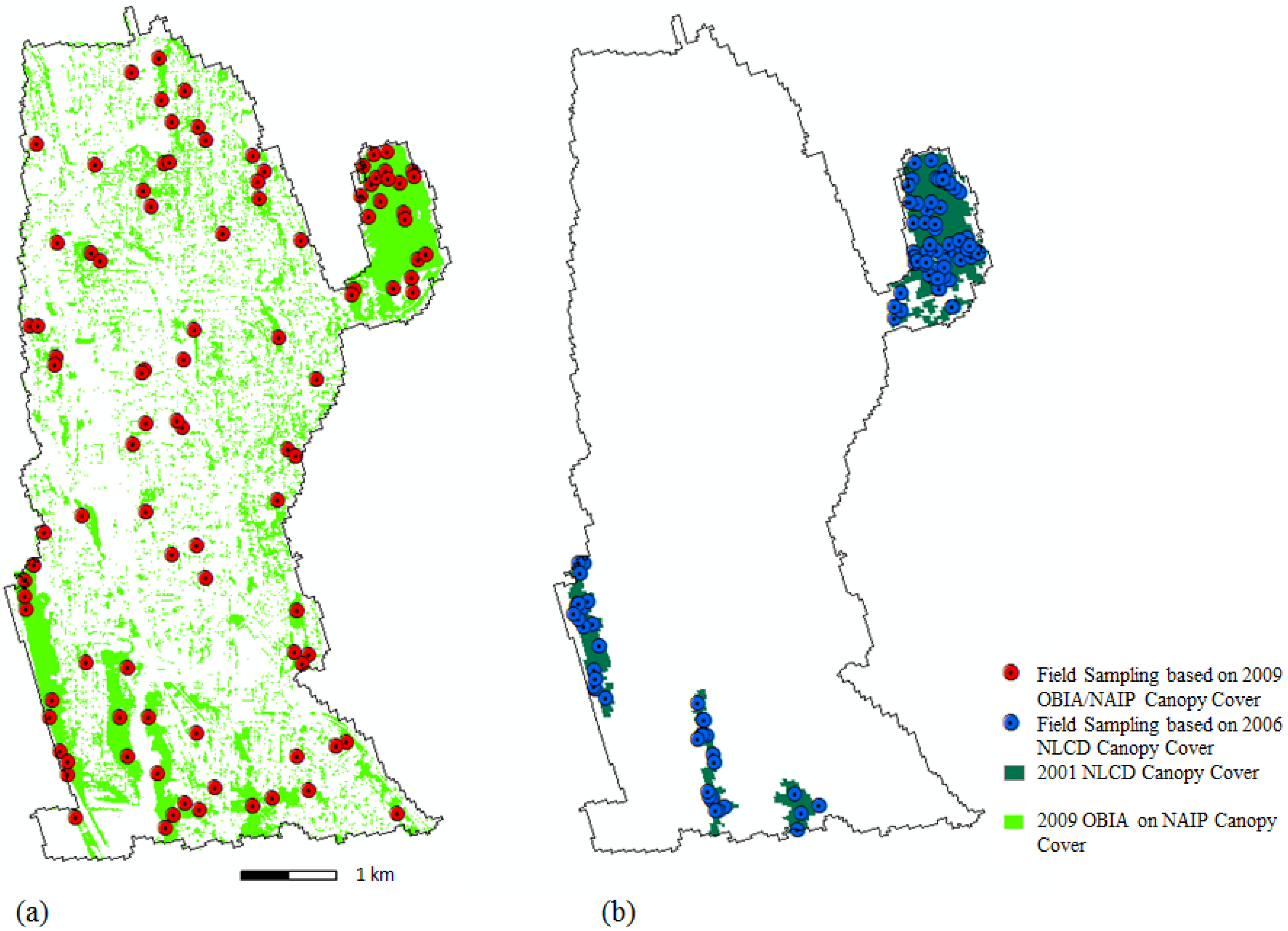A range of software solutions capable of the OBIA approach is available; further study looking into open-source vs. proprietary solutions would be valuable. Although OBIA analysis is resource intensive, requiring large data storage and processing capabilities, these issues could be resolved through a consortia approach where partners off-set some of these costs because a significant cost of production comes from fixed costs (e.g., algorithm development). A consortia approach would take advantage of economies of scale and lower production costs through replication of the algorithm over greater extents. Partnership in field data acquisition [15,38], using sampling design derived from hyperspatial data, can aid in the validation of these heterogeneous datasets; this role could potentially rely on citizen science/public involvement [39].

References

1. Clark, J.R.; Matheny, N.P.; Cross, G.; Wake, V. A model of urban forest sustainability. J. Arboricul. 1997, 23, 17–30. [Google Scholar]
2. Kerr, J.T.; Ostrovsky, M. From space to species: Ecological applications for remote sensing. Trends Ecol. Evol. 2003, 18, 299–305. [Google Scholar] [CrossRef]
3. Fassnacht, K.S.; Cohen, W.B.; Spies, T.A. Key issues in making and using satellite-based maps in ecology: A primer. Forest Ecol. Manage. 2006, 222, 167–181. [Google Scholar] [CrossRef]
4. Styers, D.M.; Chappelka, A.H.; Marzen, L.J.; Somers, G.L. Developing a land-cover classification to select indicators of forest ecosystem health in a rapidly urbanizing landscape. Landscape Urban Plan. 2010, 94, 158–165. [Google Scholar] [CrossRef]
5. Pickett, S.T.A.; Cadenasso, M.L.; Grove, J.M.; Boone, C.G.; Groffman, P.M.; Irwin, E.; Kaushal, S.S.; Marshall, V.; McGrath, B.P.; Nilon, C.H.; et al. Urban ecological systems: Scientific foundations and a decade of progress. J. Environ. Manage. 2010, 92, 331–362. [Google Scholar] [CrossRef] [PubMed]
6. Herold, M.; Couclelis, H.; Clarke, K.C. The role of spatial metrics in the analysis and modeling of urban land use change. Comput. Environ. Urban Syst. 2005, 29, 369–399. [Google Scholar] [CrossRef]
7. Hunsinger, T.; Moskal, L.M. Half a Century of Spatial & Temporal Landscape Changes in the Finley River Basin, Missouri. In Proceedings of Association of American Geographers Annual Conference, Denver, CO, USA, 5–9 April 2005.
8. Turner, M.G.; Gardner, R.H. Quantitative Methods in Landscape Ecology; Springer-Verlag: New York, NY, USA, 1991. [Google Scholar]
9. Moskal, L.M.; Dunbar, M.D.; Jakubauskas, M.E. Visualizing the forest: A forest inventory characterization in the yellowstone national park based on geostatistical models. In A Message from the Tatras: Geographical Information Systems & Remote Sensing in Mountain Environmental Research; Widacki, W., Bytnerowicz, A., Riebau, A., Eds.; Jagiellonian University Press: Kraków, Poland, 2004; pp. 219–232. [Google Scholar]
10. Anderson, J.R.; Hardy, E.E.; Roach, J.T.; Witmer, R.E. A Land Use and Land Cover Classification System for Use with Remote Sensor Data; Geological Survey Professional Paper 964; US Geological Survey: Washington, DC, USA, 1976.
11. Blaschke, T. Object based image analysis for remote sensing. ISPRS J. Photogramm. 2010, 65, 2–16. [Google Scholar] [CrossRef]
12. Cleve, C.; Kelly, M.; Kearns, F.R.; Moritz, M. Classification of the wildland–urban interface: A comparison of pixel- and object-based classifications using high-resolution aerial photography. Comput. Environ. Urban Syst. 2008, 32, 317–326. [Google Scholar] [CrossRef]
13. Zhou, W.; Troy, A. An object-oriented approach for analysing and characterizing urban landscape at the parcel level. Int. J. Remote Sens. 2008, 29, 3119–3135. [Google Scholar] [CrossRef]
14. Environmental Action Agenda 2005; City of Seattle: Seattle, WA, USA, 2005; Available online: http://www.cityofseattle.net/environment/ActionAgenda.htm (accessed on 10 October 2010).
15. Parlin, M. Seattle, Washington Urban Tree Canopy Analysis Project Report: Looking Back and Moving Forward; Native Communities Development Corporation: Colorado Springs, CO, USA, 2009; p. 17. [Google Scholar]
16. Chambers, J.Q.; Asner, G.P.; Morton, D.C.; Anderson, L.O.; Saatchi, S.S.; Espírito-Santo, F.D.B.; Palace, M.; Souza, C., Jr. Regional ecosystem structure and function: Ecological insights from remote sensing of tropical forests. Trends Ecol. Evol. 2007, 22, 414–423. [Google Scholar] [CrossRef] [PubMed]
17. Nowak, D.J.; Rowntree, R.A.; McPherson, E.G.; Sisinni, S.M.; Kermann, E.R.; Stevens, J.C. Measuring and analyzing urban tree cover. Landscape Urban Plan. 1996, 36, 49–57. [Google Scholar] [CrossRef]
18. Tuominen, S.; Pekkarinen, A. Performance of different spectral and textural aerial photograph features in multi-source forest inventory. Remote Sens. Environ. 2005, 94, 256–268. [Google Scholar] [CrossRef]
19. Foster, B. Some urban measurements from landsat data. Photogramm. Eng. Remote Sensing 1995, 48, 139–151. [Google Scholar]
20. Alberti, M.; Weeks, R.; Coe, S. Urban land cover change analysis in central puget sound. Photogramm. Eng. Remote Sensing 2004, 70, 1043–1052. [Google Scholar] [CrossRef]
21. Platt, R.V.; Rapoza, L. An evaluation of an object-oriented paradigm for land use/land cover classification. The Professional Geogr. 2008, 60, 87–100. [Google Scholar] [CrossRef]
22. Hay, G.J.; Castilla, G.; Wulder, M.A.; Ruiz, J.R. An automated object-based approach for the multiscale image segmentation of forest scenes. Int. J. Appl. Earth Obs. Geoinf. 2005, 7, 339–359. [Google Scholar] [CrossRef]
23. Halabisky, M.; Moskal, L.M.; Hall, S.A. Object-based classification of semi-arid wetlands. J. Appl. Remote Sens. 2011, 5, 13. [Google Scholar] [CrossRef]
24. Gertsch, S. Census Bureau: 98118 the Most Diverse Zip Code in US; KOMOnews: Seattle, WA, USA, 2010. [Google Scholar]
25. Wilson, G.W. Opinion: America’s most diverse zip code shows the way. Rainier Valley Post, 31 March 2010. [Google Scholar] [CrossRef]
26. Heynen, N.; Perkins, H.A.; Roy, P. The political ecology of uneven urban green space. Urban Affairs Rev. 2006, 42, 3–25. [Google Scholar] [CrossRef]
27. Xian, G.; Homer, C.; Fry, J. Updating the 2001 national land cover database impervious surface products to 2006 using landsat imagery change detection methods. Remote Sens. Environ. 2009, 113, 1133–1147. [Google Scholar] [CrossRef]
28. Definiens AG. Definiens Developer 7 Reference Book; Definiens AG: Munich, Germany, 2007; p. 195. [Google Scholar]
29. Moskal, L.M.; Franklin, S.E. Multi-layer forest stand discrimination with spatial co-occurrence texture analysis of high spatial detail airborne imagery. Geocarto Int. 2002, 17, 55–68. [Google Scholar] [CrossRef]
30. Congalton, R.G.; Green, K. Assessing the Accuracy of Remotely Sensed Data: Principles and Practices, 2nd ed.; CRC Press, Taylor & Francis Group: Boca Raton, FL, USA, 2009; p. 183. [Google Scholar]
31. Chen, Y.; Su, W.; Li, J.; Sun, Z. Hierarchical object oriented classification using Very High Resolution imagery and lidar data over urban areas. Adv. Space Res. 2009, 43, 1101–1110. [Google Scholar] [CrossRef]
32. Ke, Y.; Quackenbush, L.J.; Im, J. Synergistic use of quickbird multispectral imagery and lidar data for object-based forest species classification. Remote Sens. Environ. 2010, 114, 1141–1154. [Google Scholar] [CrossRef]
33. Erdody, T.L.; Moskal, L.M. Fusion of lidar and imagery for estimating forest canopy fuels. Remote Sens. Environ. 2010, 114, 725–737. [Google Scholar] [CrossRef]
34. Guindon, B.; Zhang, Y.; Dillabaugh, C. Landsat urban mapping based on a combined spectral-spatial methodology. Remote Sens. Environ. 2004, 92, 218–232. [Google Scholar] [CrossRef]
35. Walker, J.S.; Briggs, J.M. An object-oriented approach to urban forest mapping in Phoenix. Photogramm. Eng. Remote Sensing 2007, 73, 577–583. [Google Scholar] [CrossRef]
36. Zhou, W.; Troy, A. Development of an object-based framework for classifying and inventorying human-dominated forest ecosystems. Int. J. Remote Sens. 2009, 30, 6343–6360. [Google Scholar] [CrossRef]
37. Price, J. Spectral band selection for visible-near infrared remote sensing: Spectral-spatial resolution tradeoffs. IEEE Trans. Geosci. Remote Sens. 1997, 35, 1277–1285. [Google Scholar] [CrossRef]
38. Nowak, D.J.; Crane, D.E.; Stevens, J.C.; Hoehn, R.E.; Walton, J.T.; Bond, J. A ground-based method of assessing urban forest structure and ecosystem services. Arboricul. Urban Forest. 2008, 34, 347–358. [Google Scholar]
39. Goodchild, M. Citizens as sensors: The world of volunteered geography. GeoJournal 2007, 69, 211–221. [Google Scholar] [CrossRef]