Article

Eucalyptus Biomass and Volume Estimation Using Interferometric and Polarimetric SAR Data

National Institute for Space Research-INPE, Av. dos Astronautas, 1758, P.O. BOX 515, 12227-010 São José dos Campos, SP, Brazil
*
Author to whom correspondence should be addressed.
Remote Sens. 2010, 2(4), 939-956; https://doi.org/10.3390/rs2040939
Submission received: 21 December 2009 / Revised: 22 March 2010 / Accepted: 23 March 2010 / Published: 31 March 2010

Abstract

:
This work aims to establish a relationship between volume and biomass with interferometric and radiometric SAR (Synthetic Aperture Radar) response from planted Eucalyptus saligna forest stands, using multi-variable regression techniques. X and P band SAR images from the airborne OrbiSAR-1 sensor, were acquired at the study area in the southeast region of Brazil. The interferometric height (Hint = difference between interferometric digital elevation model in X and P bands), contributed to the models developed due to fact that Eucalyptus forest is composed of individuals whose structure is predominantly cylindrical and vertically oriented, and whose tree heights have great correlation with volume and biomass. The volume model showed that the stand volume was highly correlated with the interferometric height logarithm (Log10Hint), since Eucalyptus tree volume has a linear relationship with the vegetation height. The biomass model showed that the combination of both Hint2 and Canopy Scattering Index—CSI (relation of σ°VV by the sum of σ°VV and σ°HH, which represents to the canopy interaction) were used in this model, due to the fact that the Eucalyptus biomass and the trees height relationship is not linear. Both models showed a prediction error of around 10% to estimate the Eucalyptus biomass and volume, which represents a great potential to use this kind of technology to help establish Eucalyptus forest inventory for large areas.

1. Introduction

Recently Eucalyptus plantations mainly to produce cellulose have been increasing in SE Brazil, and to a certain extent this kind of culture contributes to carbon capture and prevents native forest exploitation. This production process needs a continuous inventory, which must be carried out once a year, being a very time consuming job and its results are an extrapolation of the measurement of some small transects. In some cases, if the plantation is suffering from some pathology and/or if it has gaps, the ground inventory might be difficult to perform. The biomass inventory is very important for the initial growing phase mainly to monitor plagues, while the volume inventory is useful to identify the right moment to cut down the trees.
The use of optical and Lidar remote sensing for surveying is a technique available in great number of countries, but currently it is a process very difficult to carry out in some Brazilian regions due to the cloudy weather, making it a slow process for large areas. The microwave remote sensing techniques for surveying have swiftly developed in the last years, using mainly the polarimetric and/or the interferometric approach, aiming to estimate the relations of biomass and volumetric contents of natural forest. Some studies using SAR (Synthetic Aperture Radar) data have been performed to map the Amazon rainforest. These studies have used a digital elevation model (DEM) by SAR interferometry, derived from X- and P-bands DEMs, in combination with radar backscatter values to estimate the forest aboveground biomass using statistical modeling, as well as to characterize forest areas with timber logging and different features at the successional stages [1,2].
The main goal of this article is to generate an estimation model of biomass and volume from Eucalyptus stands using multivariate analysis and polarimetric P-band data, as well as interferometry of X- and P-bands, in order to have a method that enables annual forest monitoring for cellulose exploitation for large areas.

2. Background

Many studies have been carried out to estimate forest biophysical parameters using SAR radiometry and polarimetry. Based on these studies five kinds of backscatter were identified due to vegetation target response; from the interaction on top of the canopy, from the interior of the canopy (volumetric backscatter), from the soil above the vegetation, from the interaction of soil and trunk, and from the shadowing effect [3]. These effects can vary depending on radar wavelength, target texture, moisture, and structure as well as on vegetation orientation.
The correlation coefficient between backscatter and biophysical parameters of a Pinus forest at P-band and L-band in different polarizations, pointed out that P-band backscatter was better than that of L-band to estimate the biomass of branches, trunks, needles and total biomass, despite the fact that the L-band cross-polarized signal showed a similar response if compared with that of P-band [4]. According to the studies in [5], the cross-polarized P-band presented the best correlation coefficient between backscatter and volume of a Pinus forest, and some saturation occurred at the backscatter response from the measured biomass. For C-band, this saturation occurred around 50 t/ha, and for L-band around 70 t/ha. During the studies reported in [6], a backscatter saturation for P-band was verified for the biomass around 100 t/ha in broadleaf and coniferous forests, with the lowest backscatter values for HV polarization if compared with the other polarizations. Studies developed by [2,7,8], observed a P-band backscatter saturation for volume of around 250 m3/ha of tropical and coniferous forests.
Some indexes like BMI, VSI, CSI and ITI [9] derived from polarimetric SAR data were developed in which a correlation was noticed in relation to some special forest parameters. The BMI index is associated to biomass, VSI is associated to volume, CSI is associated to canopy, and ITI (Interaction Index) is used to identify single or double bounce interaction. The Equations 1–4 show the equations of the indexes:
C S I = σ V V o σ V V o + σ H H o
B M I = σ V V o + σ H H o 2
V S I = σ H V o + σ V H o σ V V o + σ H H o + σ H V o + σ V H o
ITI = Phase difference between HH and VV complexes images
The interferometric coherence obtained by both ERS-1 and ERS-2 satellites, pointed out that this technique could help target discrimination [10]. It was noticed that deciduous and coniferous forests had the same backscatter intensity but different coherence, due to the fact that the autumn season caused leaf loss of deciduous forests, and thus the coherence in the C-band increased. Raney [11] explains in detail the technical definitions about interferometry, interferometric coherence, radar backscatter, and image format used by the authors in this paper.
According to studies based on Pauli decomposition [12], covariance, coherence matrixes, entropy, anisotropy, and alpha angle were obtained in order to describe kinds of target mean scattering mechanisms like the sum of all independent scatter elements. These authors described the different scattering behavior by zones in the graph of alpha angle versus entropy. These zones can identify double bounce, dipoles and surface interaction mechanisms, whose identification will depend on the kind of forest and on the radar band used.
Studies using AIRSAR data [13,14], verified that for coniferous forest, the P-band beam showed a lower attenuation by the forest components if compared to that of the C and L-bands. This happened because the P-band beam penetration was high, and the correlation coefficient in relation to trunks was higher when compared to the other band used. More recent comparative studies [15] of different sensors for pine and hardwood forest mapping showed that P-band signal from GeoSAR sensor had great interaction with trunks and soil, and the employment of interferometry in X-band for the vegetation height was more efficient for pine forests, since pine has a simpler structure than hardwood.
IHS combination of the P-band coherence, interferometric height (Hint) (Hint = difference between interferometric digital elevation model in X and P bands ) and X-band image, improved the distinction between primary and secondary forest, increasing the classification confidence rate in a tropical forest area in Pará State during the Aerosensing Radarsysteme campaign [16]. Using the same images from Pará State, the aerial biomass for secondary and primary forest of Tapajós National Forest was estimated by a third-order polynomial function based on statistical analysis [2]. The HH and HV polarizations in P-band, showed higher correlation to biomass with a higher determination coefficient (r2 = 0.77) than those at VV polarization (r2 = 0.59). Studies combining radiometric response in P band, HH polarization and interferometric data using X-band and P-band, could obtain a highly accurate prediction model to estimate the forest height in Pará State-Brazil, because the height estimation by interferometry does not suffer a saturation effect like that by radiometry [1].
Models to estimate DBH and height of Eucalyptus trees using SAR interferometry and radiometry were developed by [17], based on [1,2,16] methodologies. According to these authors, the higher wavelength P band radiometry wasn’t as efficient as the interferometry to estimate the dendrometric parameters studied. The regression models obtained for DBH and for vegetation height used a combination of P-band coherence in VV polarization and Log10Hint variables, which obtained 84 to 88% of determination coefficient in relation to the forest area inventory.

3. Area under Study

To develop this work, a reforested area was selected close to INPE’s headquarter, located in the corner coordinates 22°53′22″S 45°26′16″W and 22°53′22″S 45°26′16″W, in Pindamonhangaba district, São Paulo State/Brazil. The area under study is formed by 6.1 year old seminals of Eucalyptus saligna stands, spaced 3 × 2 meters, with 23.33 meters mean height. This area, which comprising 128.64 hectares, is named CP4 by the forestation company. The image in the Figure 1 shows the study area and the plot positions.
Figure 1. Study area and the inventory stands.
Remotesensing 02 00939 g001
The Eucalyptus area was composed of two 530 to 560 meter-high plateaus with flat relief surrounded by clear pasture. This experiment was carried out during a dry period, and soil moisture was not considered in this work. In case of soil moisture increase, P band interaction between soil and trunks might change and therefore affect the estimation models, in which case, new tests will be necessary to verify to what extent it can disturb the models.

4. Methods

Several tasks were performed to obtain the microwave data, the topographic survey data and the forest inventory. The goal was to find out the relations between tree biomass, volume, with the radar response, aiming at building regression models to estimate these biophysical parameters. The block diagram of Figure 2 shows an overview of the methodological procedures used.
Figure 2. Methodological procedure diagram.
Remotesensing 02 00939 g002
Based on the statistical model, a numeric model of the biomass and volume were generated, obtaining an image whose pixel values correspond to the regression of numeric values, with one meter resolution. The IHS technique was used to visualize these final results, which combined the X band image radiometry, as I channel, and the regression model result as the H channel filtered by 21 × 21 window, while the S channel was adjusted to 50% of saturation. From the regression model, an estimated standard deviation image was obtained using the Neter [18] method, that calculates the variance estimate of a mean response using the MSE (mean square error of the regression), applying this procedure pixel by pixel of the input variable images.

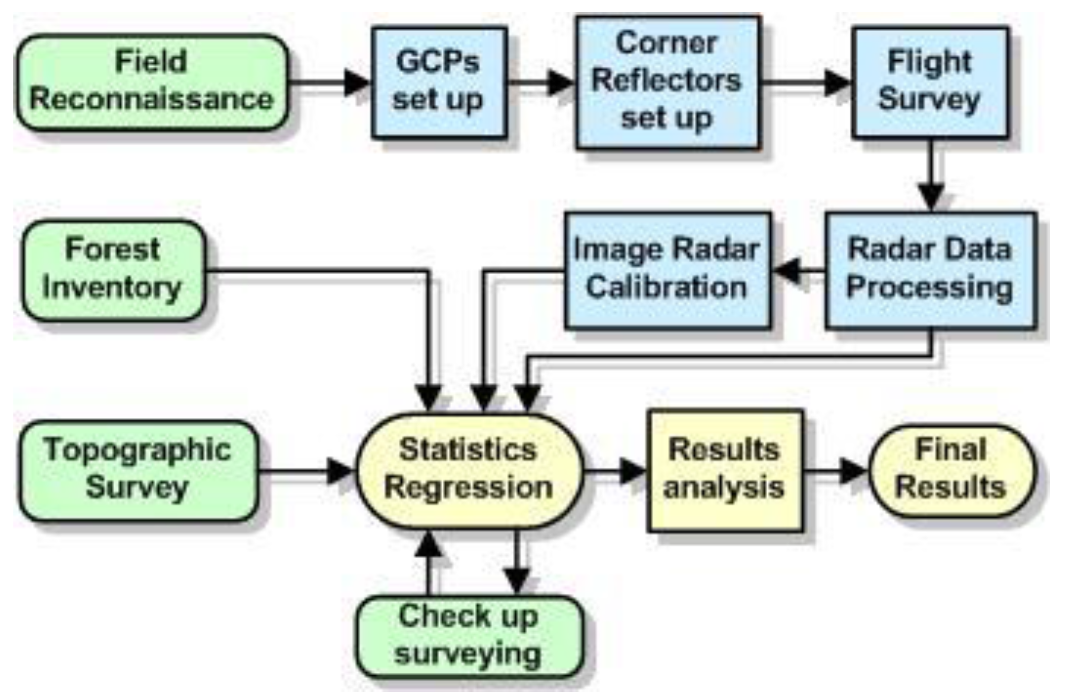
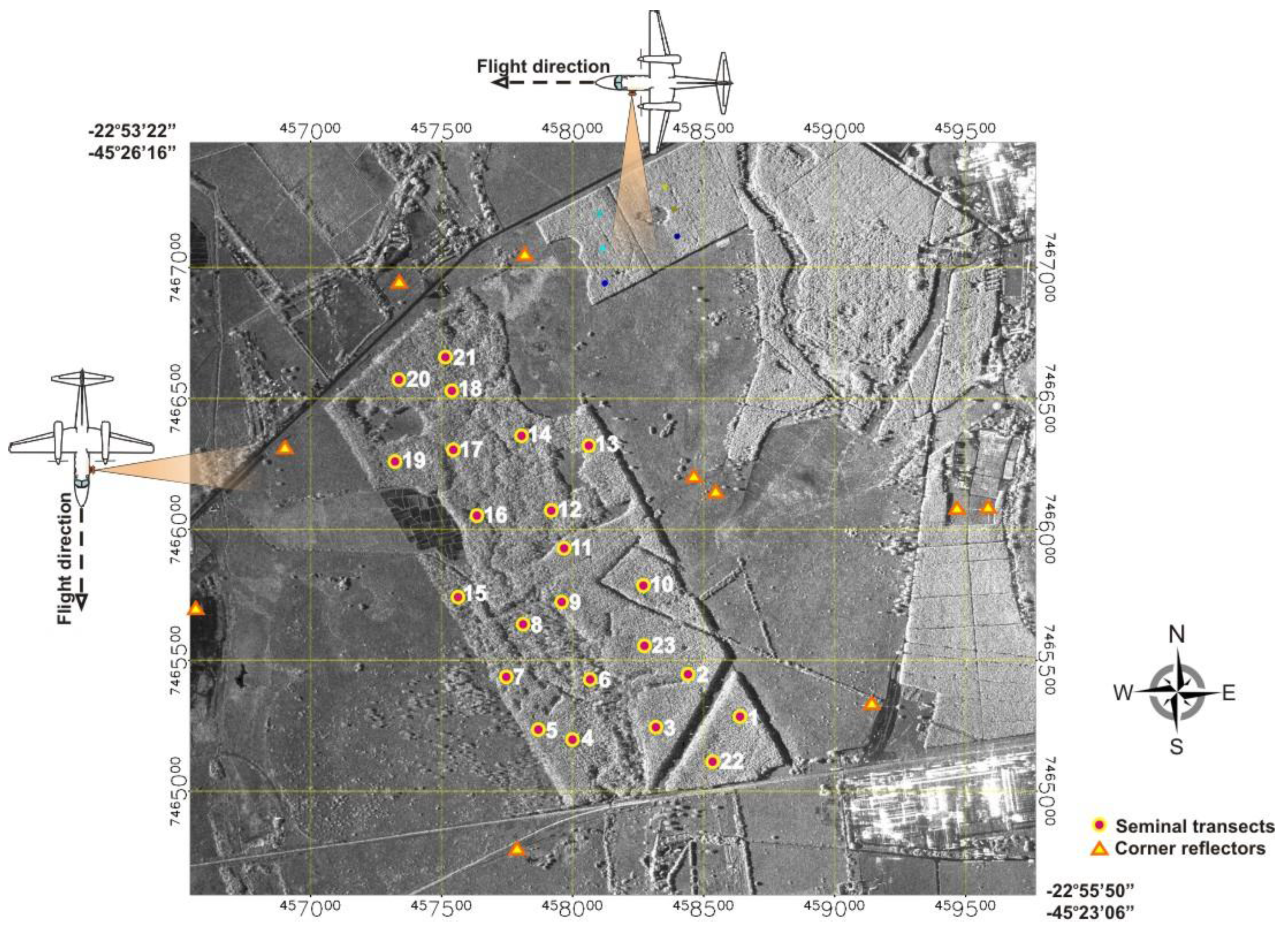
4.1. Acquisition of Field and Radar Data

The first step of the work was field reconnaissance, to locate the best areas to install the eight corner reflectors and their surroundings. The corner reflectors were used for developing the phase calibration for interferometric processing for X and P bands, as well as for radiometric calibration to obtain the σ° P band images. All the corner reflectors were 1.5 meters edge, and used for both P and X bands. Each corner reflector was installed on a GCP (Ground control point) that had been previously measured by a geodetic GPS. These GPS trackings were carried out by static relative method, using an official first order satellite base, which permitted to obtain 5.0 cm of plani-altimetric coordinate precision. Besides setting up the GCPs, it was necessary to use a high precision geographic reference point at the airport used by the airplane. This point was tracked by a geodetic GPS during the flight survey to allow the generation of the attitude vector radar by the airborne IMU (Inertial Measurement Unit) processing.
The inventory work was done simultaneously with the SAR survey in December 2004 by the Diametro Company, to characterize the dendrometric parameters according to the annual inventory. The inventory samples distribution in the study area, as well as the flight directions are illustrated on Figure 1. During the forest inventory samples were collected in 23 independent stands with ~400 m2 each, to obtain dendrometric parameters such as total height, commercial height, DBH (diameter at breast height) and aerial dry biomass. Total height represents tree height from the ground level to the tip of the tree, whereas commercial height represents bole height from the base up to the first branches. DBH, total and commercial heights were measured by conventional field inventory, and biomass was measured by destructive method. For biomass measurement the representative tree method was used, where one Eucalyptus tree whose DBH was similar to the mean of the stand was used to represent the whole stand.
Aerial dry biomass means the total tree biomass above ground level, including trunk, branches and leaves. Destructive biomass measurement method is a selective logging of a representative tree from a uniform transect. This tree selection procedure is a standard practice on forest engineering for inventory of Eucalyptus biomass plantation, that selects a representative individual from a transect to measure its biomass, whose DBH would be similar to that of mean transect [19,20]. As the plantation is the same age, composed of only one species, and with no undergrowth, this procedure is considered acceptable for biomass inventory of Eucalyptus plantation. Field inventory of volumetric data was obtained by allometric equations developed by the cellulose companies (Nobrecel and Diametro), based on DBH, total height and on form factor to estimate the Eucalyptus stem volume (Equation 5):
V o l u m e = ( D B H 2 * π 4 ) * T o t a l   H e i g h t *   F F F F = F o r m   f a c t o r
The form factor was obtained from the division of the real tree volume by the cylindrical volume; this factor was applied according to tree diametric class (Table 1).
Table 1. Form factor.
DBH (cm)FF
4.0–12.00.46
12.0–20.00.44
20.0–28.00.42
The DEM (Digital Elevation Model) was obtained by the interferometry technique using the Orbisat SAR system (OrbiSAR-1), which provided the interferometric and polarimetric data in two frequencies, X and P bands. The DEMs were obtained by two-passes for P band interferometry and one-pass for X band interferometry. Four polarizations were used at P-band, which generated four DEMs, four complex images and four interferometric coherences (CohPHH, CohPHV, CohPVH, CohPVV). X band coherence, DEM and complex image were generated in HH polarization.
Mapping flights were crossed to minimize the shadowing effect, and so the image regions which lacked information due to shadows were filled in by the Orbisat mosaic techniques. For this campaign the mapping scale was 1:25,000 for P-band and 1:10,000 for X-band, whose final pixel size was 1.0 meter for X band and 2.0 meters for P band, with the same values for the respective altimetry. X band interferometry was carried out with 2.77 meters of baseline, while for P band interferometry was necessary 50 meters of baseline.
The radar survey was carried out on December 14, 2004, at 2:00 am for a period of 72 hours of drought (0 mm/day), according to the data from the meteorological station close to the area under study, and supervised by the Brazilian center for forecast and climate studies (CPTEC). The topographic survey was carried out using a Topcon total station, model GTS-701, with 3” of accuracy. These topographic profiles were done with 10 meter spacing, covering all transects and some pasture areas. The measured starting point was the same as the one used to support the corner reflector, and as the one used in the final measurement, which allowed topographic adjustments describing a closed polygon, and obtained a 5 cm precision in the final adjustments.

4.2. Radar Data Processing

SAR images were generated with four looks and geocoded using the corresponding digital elevation models in order to obtain the orthorectified geometry. Rombach et al. [21] described the details about the Orbisat software for data transcription, IMU processing, and SAR data processing to obtain DEM, orthoimages, and coherences. Single sized corner reflectors equally distributed between near and far ranges were used, based on the methodology presented by Zink et al. [22]. The system linearity was verified by measuring the radar cross section of each corner reflector. The signal to noise ratio, the antenna pattern, radar losses and radar illumination geometry were also considered. The final radiometric accuracy was better than 1 dB. Due to the large wavelength of P band, around 72 cm, the radar cross section of a corner reflector with 1.5 m side length can’t cause saturation or non-linearities either in the analog part or in the analog to digital conversion of the radar.
The polarimetric calibration of P-band was done using Quegan methods [23]. The crosstalk processing, channel imbalance and polarimetric calibration were carried out by the corner reflectors response. After all corrections were done, the scattering decomposition took effected to obtain entropy, anisotropy and alpha images (Radar Tools software—RAT 0.16.2 version). The Pope indexes (VSI, CSI and BMI) were calculated from the P band backscatter magnitude data, and the ITI index was calculated from the backscatter phase P band data. To generate these indexes, to georeference the images, and to do region analysis, ENVI 4.2 and IDL 6.2 (Interactive Data Language) softwares were used.
All scenes were radiometrically calibrated using a methodology used by Santos [2], based on the corner reflector peak response, in order to obtain a correction factor to transform the P band amplitude images into σ° images, by software routines developed by INPE using IDL (Interactive Data Language). For this procedure the corner reflectors azimuth and elevation angles were calculated by Orbisat Company before the flight, using the flight plan and the GCP geographic coordinates. This procedure was reliable since the corner reflectors pointing direction in relation to the azimuth and elevation angles had a high accuracy (5 cm). Besides that, as the area under study is flat, the incidence angle did not present large variations.

4.3. Statistical Regression
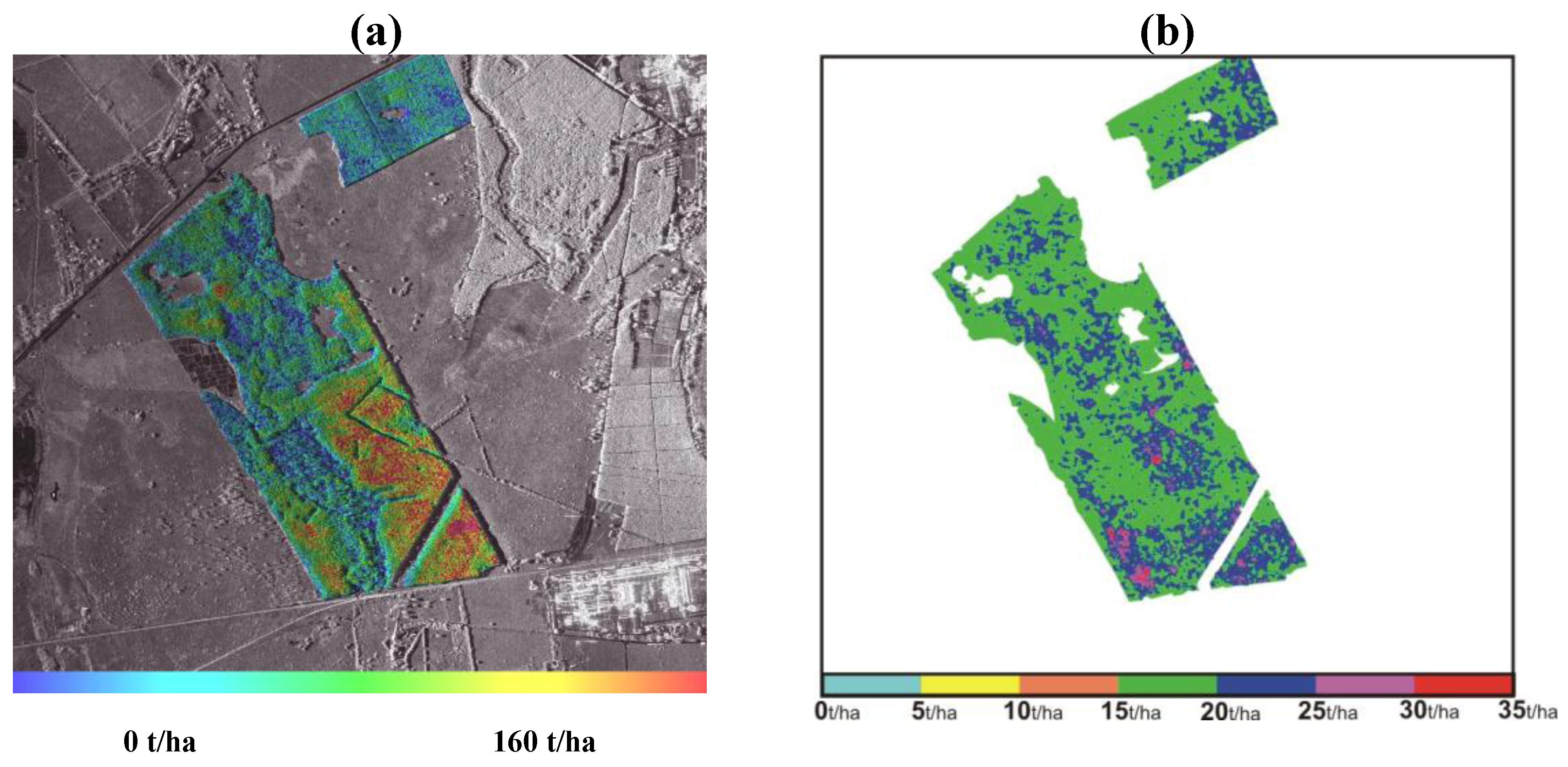
To select the set of variables that could contribute to the regression models, the determination coefficient (r2), adjusted determination coefficient (r2a), Cp criteria, and Stepwise method were used by Statistica 6.0 version software. According to studies reported in [18], it was pointed out that a high r2 value does not mean a good adjusted model for the regression model, because it depends on the number of variables involved. The r2a coefficient takes into account the number of explicative variables in relation to the number of observations. So while r2 coefficient increases with the number of variables, r2a doesn’t show this behavior, making it more relevant than the r2 coefficient. The Cp criteria involve the total mean quadratic error of each regression adjusted model subset, in which each adjusted value variance is considered a bias. With the Cp criteria it is possible to identify dependent variable subsets, whose mean quadratic error is low, i.e., when the Cp value is similar to parameter numbers (p), it means that the model has a lower bias.
The Stepwise method consists of a computational analysis that starts with a constant without any interest variables, and at each step, after adding a new variable, the possibility to extract it from the model is tested in case its contribution is not considered significant, and variables introduced in the model at a certain step, do not necessarily remain until the end of the process. For the evaluation of the residual variance constancy of the regression variables, the Levene test was used to compare two subsets of the data samples, in order to determine if the absolute deviation mean from one subset differs from the other one. For the outlier tests, the Cook distance test was used. It considers the influence of a certain observation in face of other adjusted values. This influence is measured by the percentile from an F distribution. According to studies in [18], a 10 to 20% range would be the limit for a sample to be considered an outlier. For multi-colinarity evaluation, the VIF (Value of Inflation of Variance) criterion was used. This criterion computes the impact over the variance of each variable as a consequence of the correlations of other present regressors. Some studies pointed out that VIF values above to 10 are a multi-colinarity indication [18].
For the prediction model evaluation, the PRESS (prediction sum of squares) is suggested by Neter [18] in cases where the number of samples is small, making it impossible to use a subset as a control group (leave-one-out cross validation). This criterion eliminates the ith case from the data set, and estimates the regression function with the remaining observations, and then uses this regression equation to estimate the predicted value. The quadratic sum of the n prediction errors defines the PRESS value. According to Neter [18], when the values of PRESS and SSE (Sum of squares error) are similar, the MSE (Mean squared error) can be a reasonable index of model predictive capacity.

5. Results

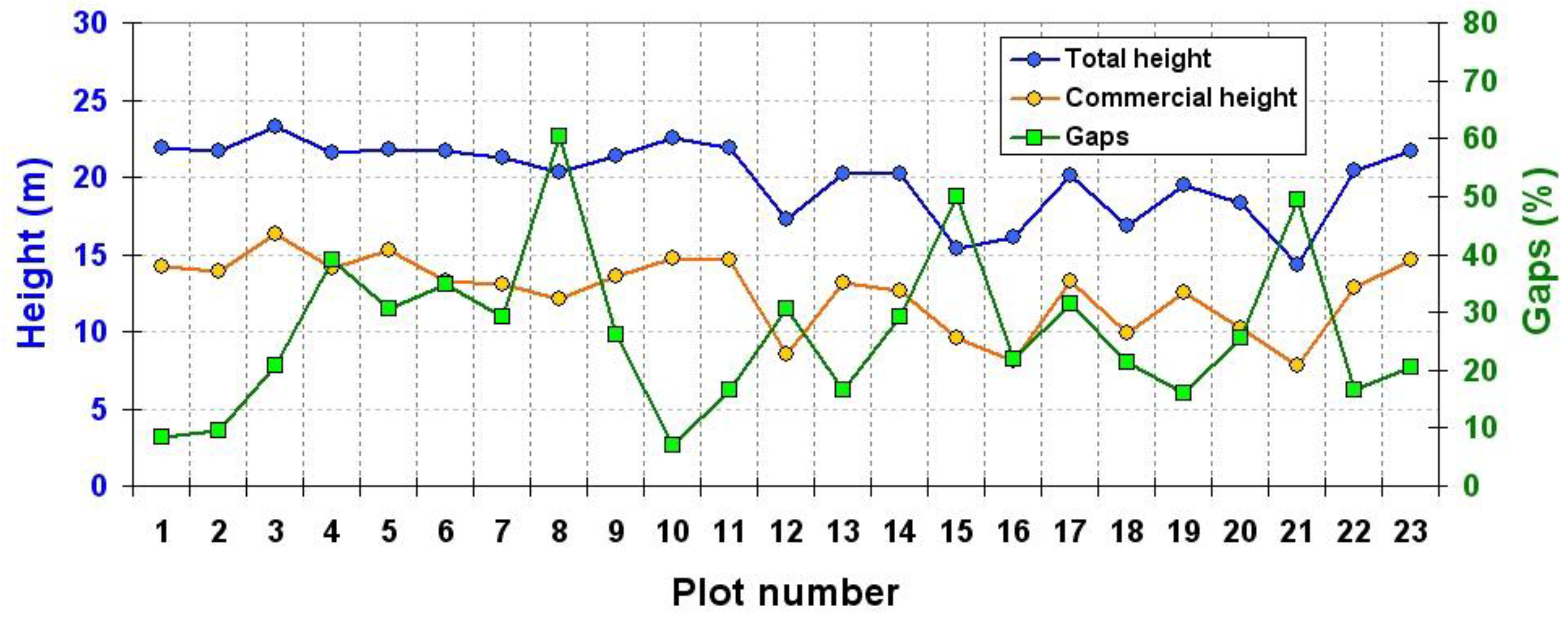
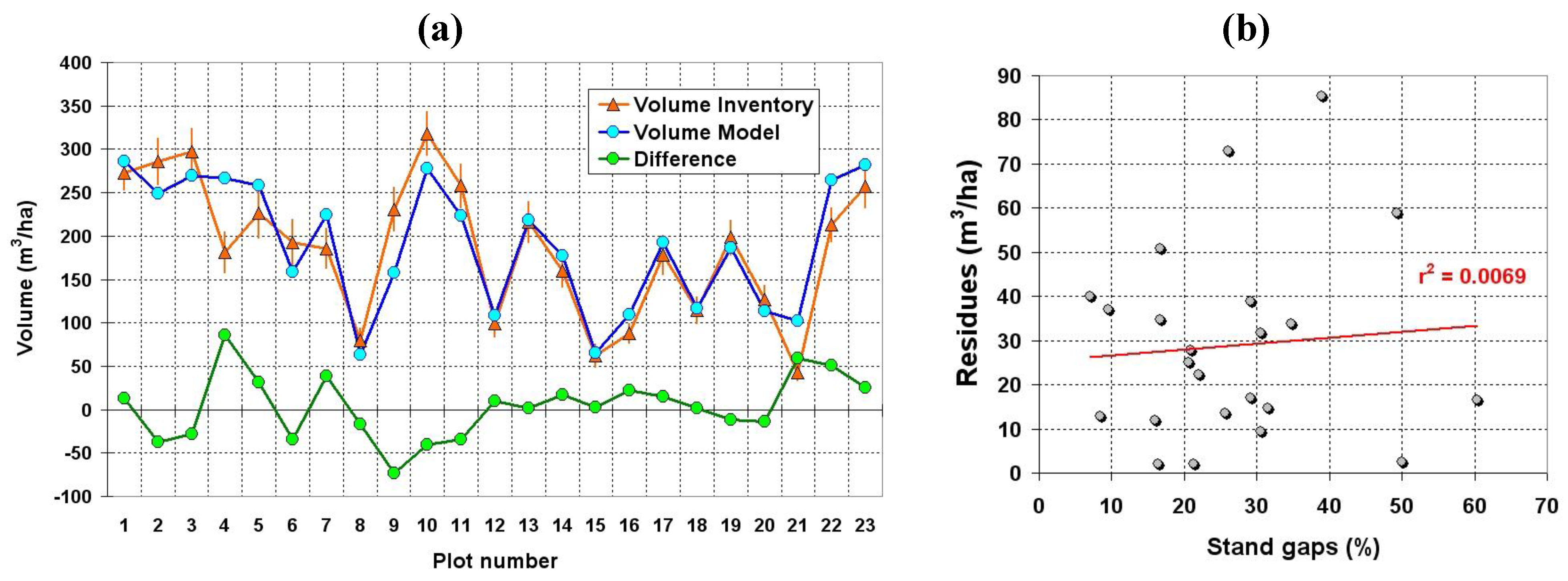
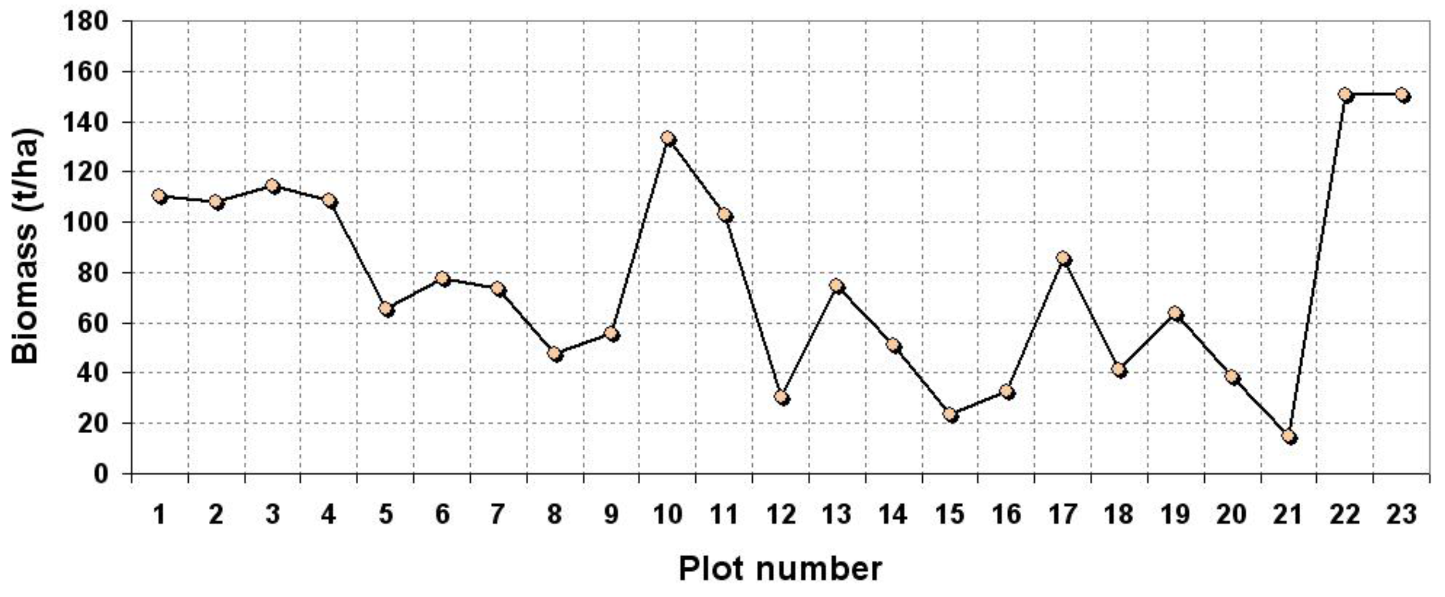
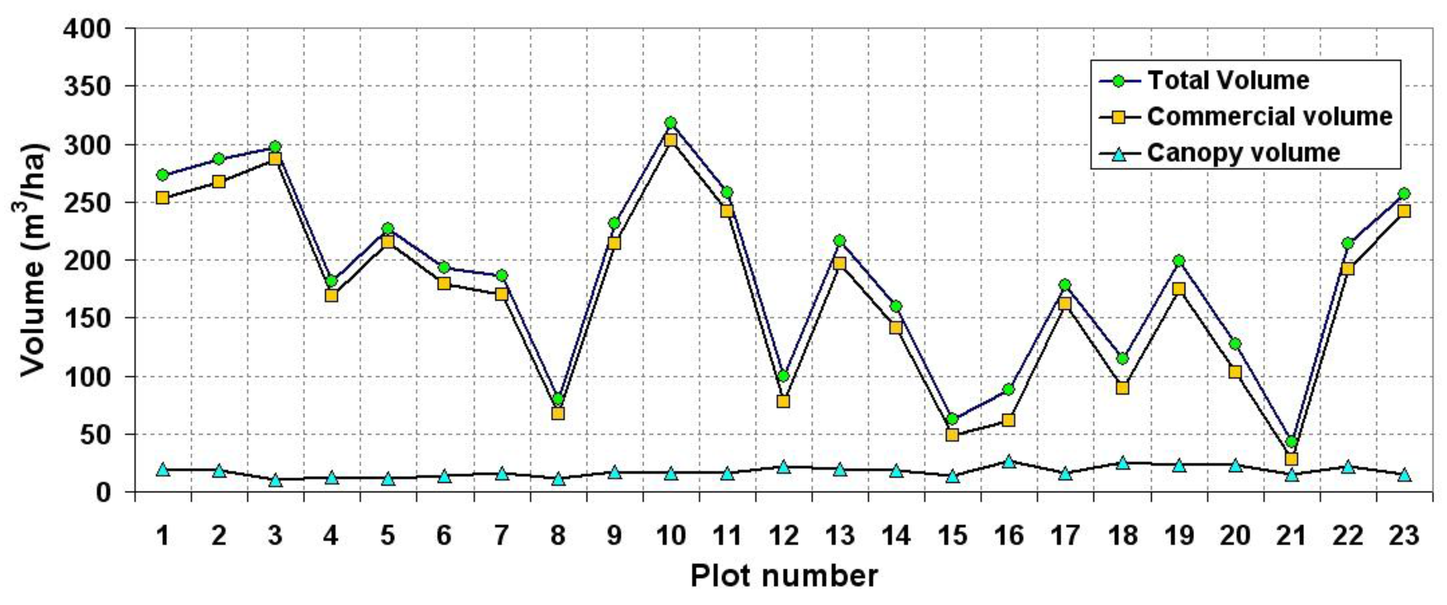
5.1. Forest Inventory
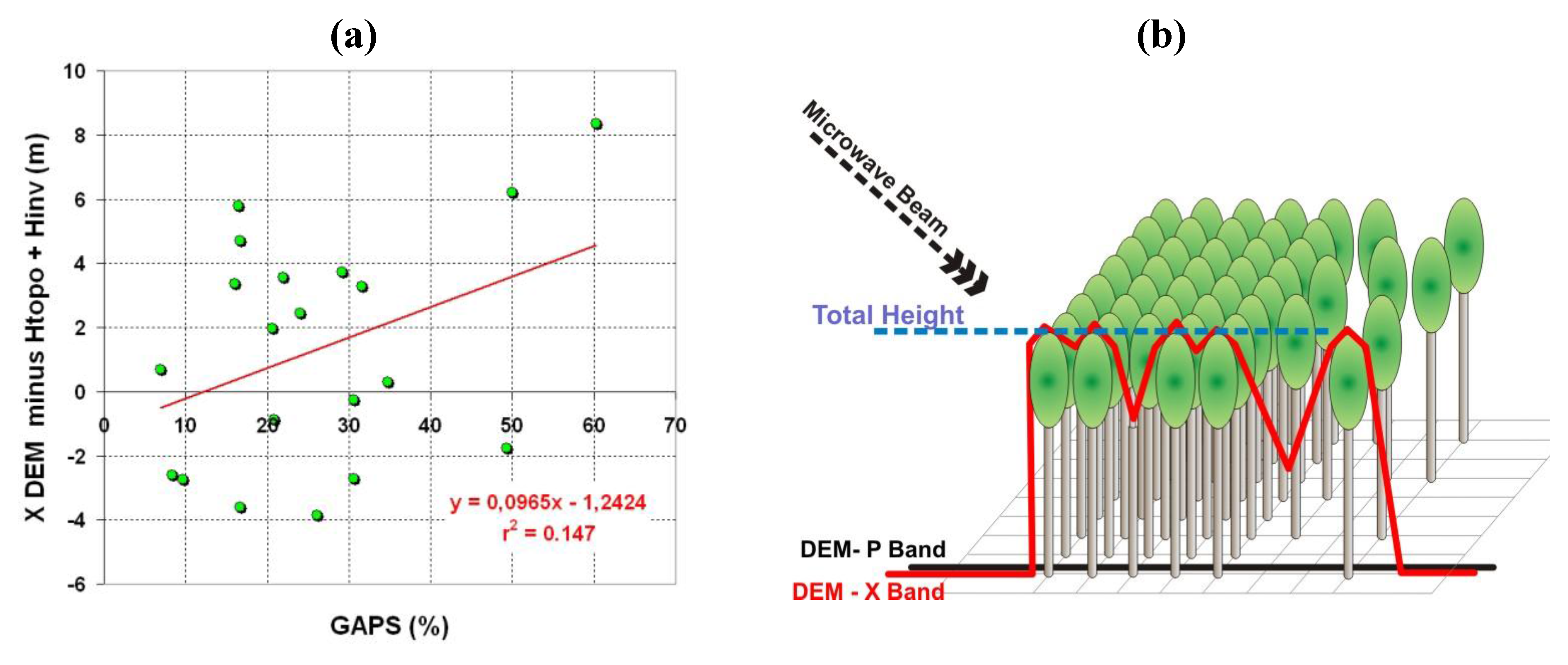
The biomass values obtained by the inventory showed a great variability (14.88 to 150.796 t/ha). These large variations happened due to edaphic problems, water availability, and genetic differences since it was a Eucalyptus seminal plantation where the trees showed differences among each other. The graph in Figure 3 shows the variability of the biomass measured for each plot number.
The tree total height measured during inventory had a large variation due to the same reasons previously explained for the biomass inventory results. Some gaps were observed inside the stands where some trees were either missing in the grid plantation or felled down. These gaps showed a percentage between 1.64% and 60.27% for the stands. The trees with bifurcation, dead, or broken were not considered as a gap according to this rule, and the green graph axis of Figure 4 shows the gap behavior for each plot number. The graph in Figure 4 illustrates the commercial and total heights, as well as the gap behavior for each plot number.
Figure 3. Biomass.
Figure 3. Biomass.
Remotesensing 02 00939 g003
Figure 4. Tree heights.
Remotesensing 02 00939 g004
The stand total volume inventory showed a high variability (43.00 to 318.13 m3/ha), while the canopy showed a low variability (15 to 30 m3/ha) with small mean volume. Total and commercial volumes (trunk volume) were very similar pointing out that trunks were the dominant structural element in the Eucalyptus stands, and as a consequence the canopy volume had to be very small. The graph in Figure 5 illustrates the total, commercial and canopy volume behavior for each plot number.
Figure 5. Total, Commercial and Canopy mean volume.
Remotesensing 02 00939 g005
A second order relationship between dry biomass and tree heights was observed during the inventory with 0.602 of determination coefficient, and a big data dispersion for the largest biomass and height values was also observed (Figure 6a). The analysis of tree volume and total height showed that point distribution was more linear than that of biomass case (Figure 6b). The regression between volume and commercial height (trunks) showed a better determination coefficient (~2% more) when compared to that of total height.
Figure 6. (a) Volume and tree heights; (b) Biomass and tree heights.
Remotesensing 02 00939 g006

DEM Quality 

The DEM assessment in forested areas, showed a standard deviation of around 1.9 meters for the PHH band, and 17.31 meters for the X band, when compared with the topographic survey data (Table 2). The comparison of topographic survey height with P band interferometric DEM showed that HH polarization was the best digital terrain model obtained, with the lowest standard deviation. On the other hand, this result suggested that the Eucalyptus trees had some interaction with the other polarizations, causing some disturbance on the interferometric DEM quality.
Table 2. DEM quality.
BandStandard deviation (m)
(Forested area)
Standard deviation (m)
(Pasture)
PHH1.96.17
PHV1.998.00
PVV2.297.68
XHH17.310.67
The comparison of the sum of the inventoried tree heights with the topographic ground measurements, and with X band DEM heights, pointed out a standard deviation around 3.37 meters. It means that X band DEM had a bigger interaction with the tree heights than that of the P band DEM. For pasture areas, the standard deviation for PHH band was 6.17 meters, while for X band was 0.67 meters. The reason for this behavior was that the terrain was flat and covered with grass, which caused a specular reflection for P band, decreasing the interferometric coherence, while increasing the X band coherence due to the grass high backscatter values.
Comparing the difference of DEM in X band and the ground truth, i.e., topographic height (Htopo) inside the stand added to inventory height (Hinv), with the percentage of the stand gaps, a determination coefficient of around 0.14 was noticed. Although this percentage was low, the tendency was a positive line graph, pointing out that the interferometric DEM errors increase with higher gap percentages (Figure 7a). This result pointed out that those gaps inside the stands affected ground DEM discrimination, whereas for the same gap percentages, a different X band DEM behavior was noticed. This is due to the fact that the gaps had different sizes and spatial distributions, which can induce intermediate height measurements which can harm the models that used this variable (Figure 7b).
Figure 7. (a) Gaps and ground truth (Htopo + Hinv); (b) DEM and gaps.
Remotesensing 02 00939 g007

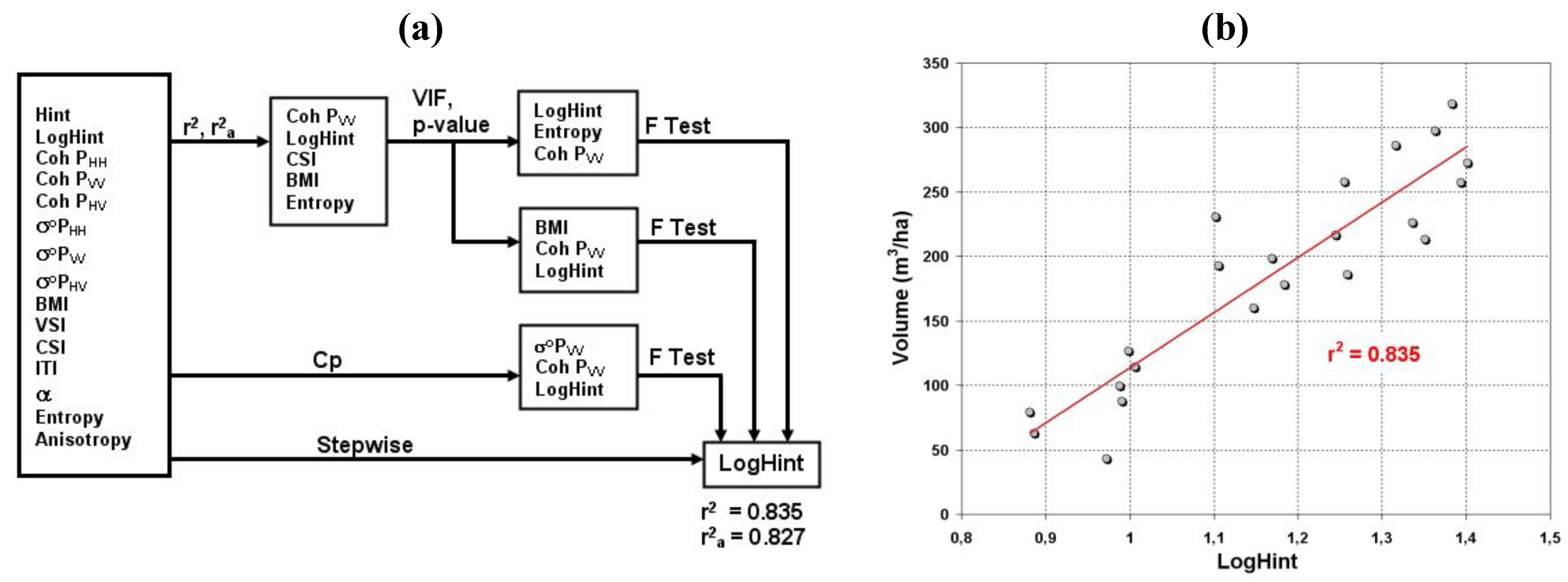
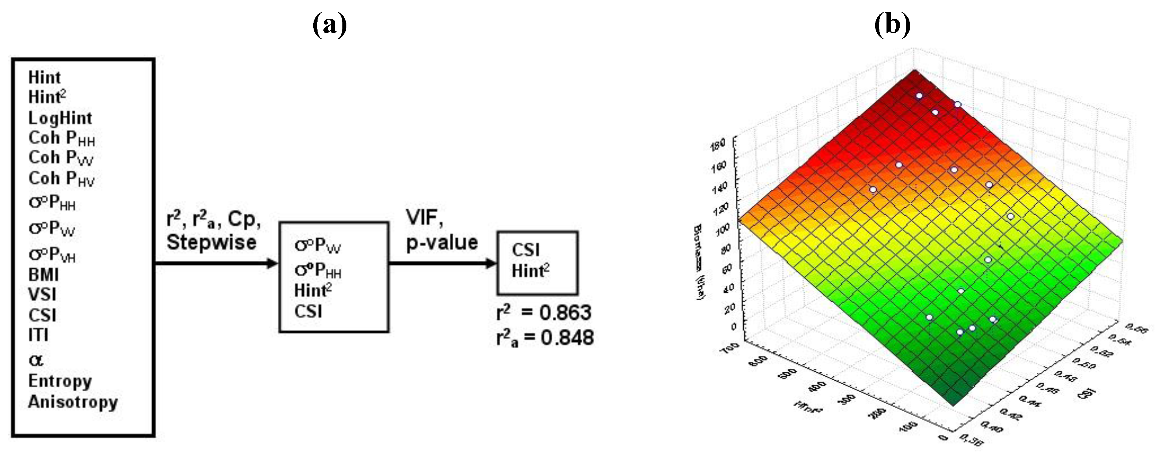
5.2. Selection of Variables for Regression Models
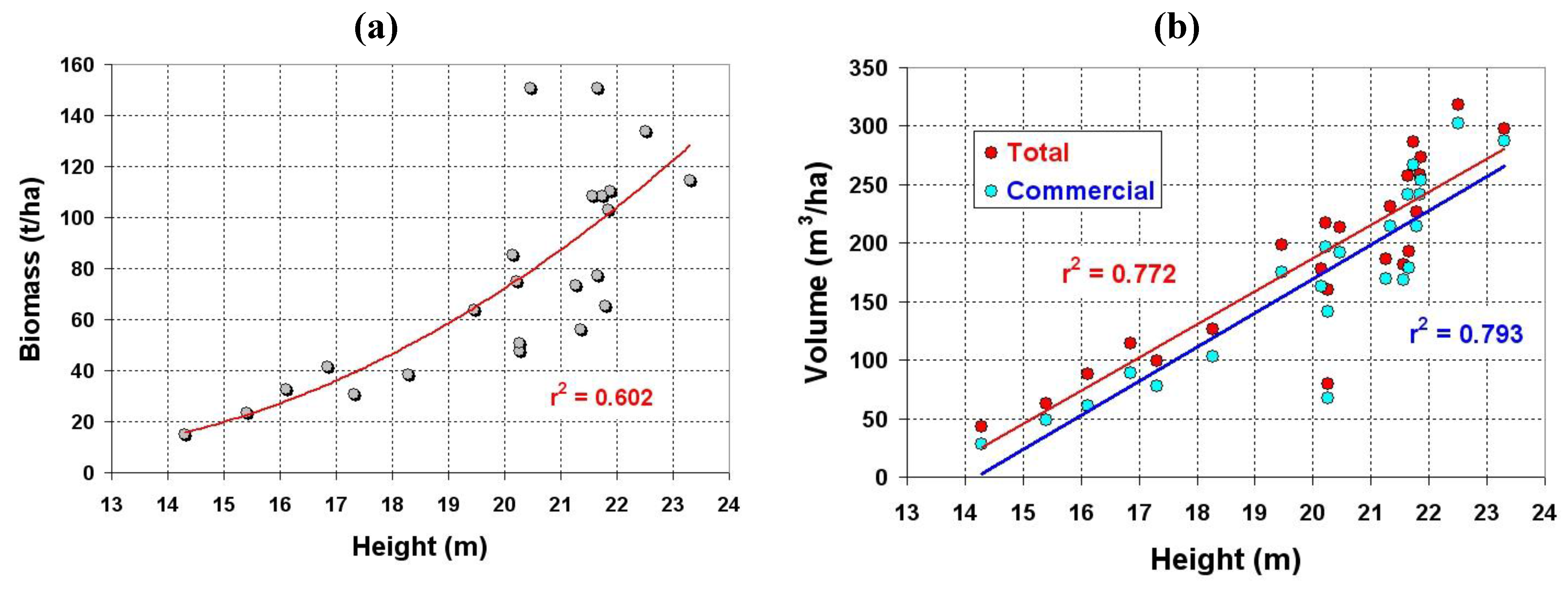
5.2.1. Volume model

Field inventory data and SAR products (interferometry/radiometry/decompositions) were used to obtain an Eucalyptus volume model. The tests for vegetation volume variable selection showed three groups of variables. The first group of variables was composed of CohPVV, Log10Hint, CSI, BMI, and Entropy which were selected by r2 and r2a criteria. The second group was selected by Cp criterion, which pointed out the variables CohPVV, Log10Hint and σ°PVV. The third group was selected by the Stepwise criterion which pointed out the variable Log10Hint.
Volumetric scattering index (VSI) was also tested, but it didn’t show statistical significance for the timber volume model, so this variable was discarded for the regression model. Similarly to the VSI index, the interferometric coherence in P and X bands presented low sensitivity to tree volume. F and VIF tests (Value of Inflation of Variance) were applied to the first and second groups, to eliminate the lower significance variables from each group. The same procedure was considered for the different groups of variables, resulting in a model formed only by the Log10Hint variable, agreeing with the Stepwise criterion result. Figure 8a illustrates the flow diagram with the initial variables and the groups selected by the statistical tests, and the final volume model is shown by Equation 6:
Volume = −314.035 + 427.946 Log10Hint
This model obtained 0.835 of determination coefficient, with one outlier case for stand 4. Figure 8b graph illustrates the volume model behavior, whose final result showed a good adjustment to the data. The farthest point from the regression straight line was due to the detected outlier (stand 4), which was not considered in the final regression model.
Figure 8. (a) Flow diagram of variables selection; (b) Graph of volume regression model.
Remotesensing 02 00939 g008
Comparing the predicted results with the inventory data, it was noticed that in some cases the model showed differences beyond the data standard deviation due to the outlier, which was discarded in the regression. Moreover, the gap percentage in the stands was between 6.9 to 60.3%, which disturbed the interferometric height by SAR sensor. The comparison with model result and inventory data and their correspondent differences are illustrated on Figure 9a.
Figure 9. (a) Comparative graph between inventory volume, volume regression model results and difference between the ground truth and the model (Difference); (b) graphic of regression residues and percentage of stand gaps.
Remotesensing 02 00939 g009
The largest difference between the model result and inventory data occurred in stand 4. This result was considered as an outlier during the regression tests so it was not used to build the final regression model, and its main characteristic was the great number of gaps in this stand (38.89%) and the terrain slope which disturbed the modeling. When comparing the regression residues with the percentage of stand gaps, a low correlation among them with a great data dispersion was noticed, whose result is a low value of r2 (0.0069) (Figure 9b).
The final volume regression model pointed out that the Log10Hint was the most relevant SAR variable for this model. For the model validation, the criteria PRESS (Prediction Sum of Squares) and SSE (Errors sum of squares) were used, whose values were similar, allowing the use of MSE (Mean Squared Errors) to predict errors. The MSE for the volume regression model presented a value of 1,126.6 m6/ha2, which represented 33.56 m3/ha, or 10.55% of prediction error if compared with maximum stand volume.
Based on the statistical model, a numeric model of vegetation volume was generated, obtaining an image whose pixel values corresponds to the numeric regression values with one meter resolution. The final hypsometric image can be seen in Figure 10a, with a color scale that corresponds to tree volume. It can be observed that volume varied from 0 to 325m3/ha, and that the regions in blue color correspond to the stand gaps and to the errors in Log10Hint measurements. The standard deviation image was sliced in 10 gray levels and associated to different colors (Figure 10b).
Figure 10. (a) IHS image of vegetation volume model (I = X band image, H = vegetation volume, S = vegetation mask); (b) Standard deviation image.
Remotesensing 02 00939 g010
It can be verified that the standard deviation image had two predominant levels, 30 to 35 m3/ha and 35 to 40 m3/ha bands. These levels correspond to an estimation error between 16.1% and 21.47% (30 to 40 m3/ha), if compared to the mean tree volume (186.33 m3/ha). Comparing it to the maximum tree volume (318.13 m3/ha), the corresponding estimation error was between 9.43% and 12.57%.
For volume modeling, the Hint variable had the highest correlation with this Eucalyptus forest parameter, while the backscatter variables and its decompositions were not selected by the several statistical tests applied. The probable reason for this behavior is that Eucalyptus trees have their structure predominantly cylindrical and vertically oriented with a small crown, and so the height information is strongly correlated to the Eucalyptus volume. So for Eucalyptus volume monitoring the interferometric height (Hint) was the most efficient variable for the predictive model developed.

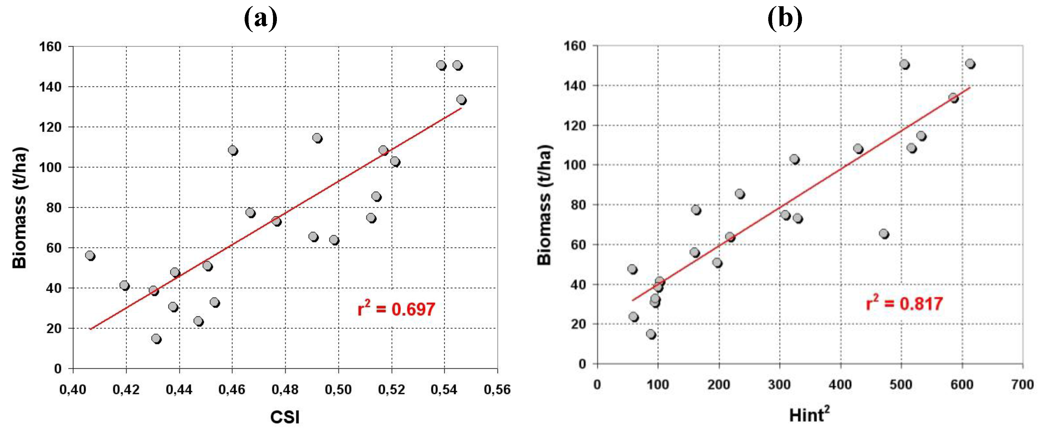
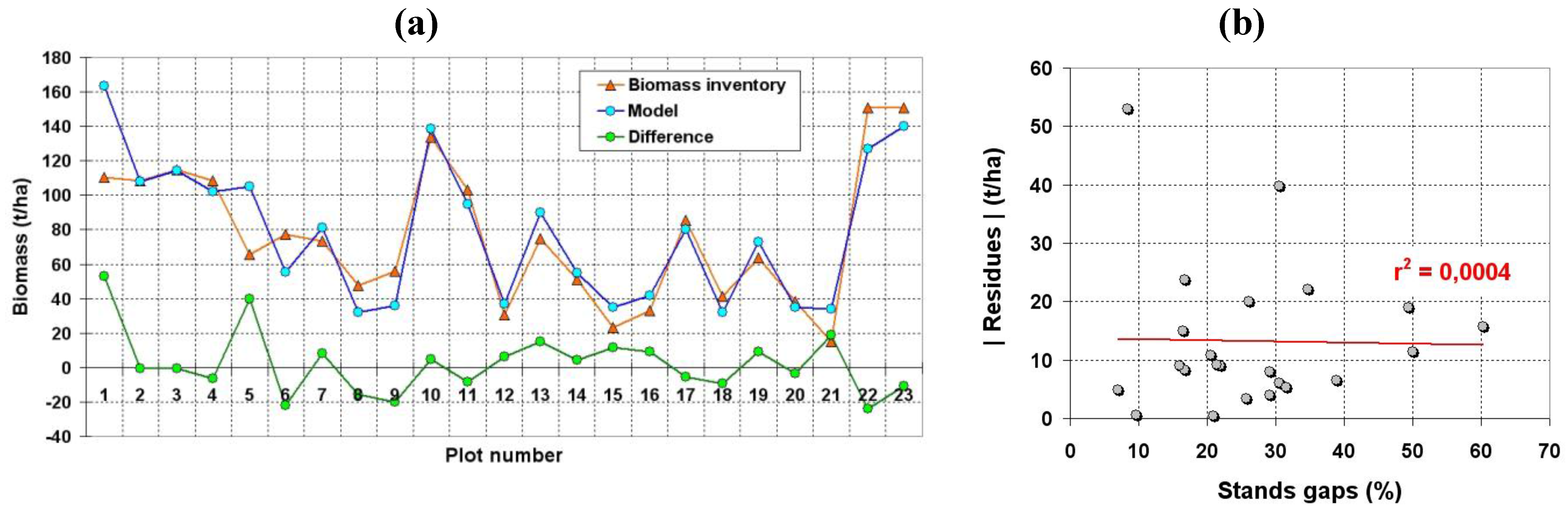
5.2.2. Biomass model

The Eucalyptus biomass model was obtained by linear regression modeling among field inventory data, interferometric/radiometric SAR data, and scattering indexes developed by [9], but only the variables CSI index, Hint2, σ°PVV and σ°PHH, were statistically significant for the biomass model. According to VIF tests and to p-value analysis, the final model used only two variables, CSI index and Hint2, with just one outlier detected, which was not used in the final regression. This stand had its biomass value much higher than that of other stands and for this reason it was considered as an outlier. The final biomass model is shown at Equation 7:
Biomass = −114.505 + 0.137 Hint2 + 316.058 CSI
The CSI variable brings the radiometry contribution of σ°PVV and σ°PHH, because it is a consequence of both data, so the biomass model was influenced by the interaction of vertical and horizontal stand elements (branches, leaves, and stems) represented by the CSI index. The squared Hint (Hint2) variable contributed to the biomass model too, since Eucalyptus biomass has a second order correlation with its height, so the squared Hint variable showed the best adjustment. The Biomass model obtained 0.863 for the determination coefficient, with one outlier case related to plot 1. The sequence diagram on Figure 11a, shows the initial and final variables used to obtain the final model, and Figure 11b graph illustrates the model behavior of the final model equation.
Figure 11. (a) Flow diagram of variables selection; (b) biomass regression model graph.
Remotesensing 02 00939 g011
Based on the inventory data, the total biomass and the total mean height showed a second order correlation between these variables, while variables Hint2 and CSI presented a linear behavior (Figure 12).
The estimated regression model values have a good similarity with the inventory data, where the estimated values were similar or coincident with the field work data. However, in some cases, some disagreements were detected, as one can observe at Figure 13a.
Figure 12. (a) Biomass and CSI; (b) Biomass and Hint2.
Remotesensing 02 00939 g012
Figure 13. (a) Comparative graph of inventoried biomass, modeled biomass, and the correspondent difference; (b) Graph of stand gaps percentage and model regression residues.
Remotesensing 02 00939 g013
Estimation errors that happened in some plots probably originated from the Hint2 and CSI measurements or from biomass measurement during the forest inventory. Other factors that could have influenced these results are the small variations of canopy water content and/or edaphic problems from each plot that could change the radar backscatter, and so disturb the CSI index, and therefore disturb the final model response. Besides that, model variables are a consequence of an average from pixels of ROIs (region of interest), and so individual or combined factors might have been responsible for the underestimation of model values for some plots.
Similar to the volume model, the analysis of the percentage of stand gaps and the biomass model residues pointed out a weak correlation (r2 = 0.0004), denoting that these variables were independent, and that the gaps didn’t disturb the model quality. Figure 13b shows the graph of stand gaps percentage and the model regression residues. For the model validation, the criteria PRESS (Prediction Sum of Squares) and SSE (Sum of squares errors) whose values were similar were used, allowing the use of MSE (Mean squared errors) to predict errors. MSE for the biomass regression model presented a value of 245 t2/ha2, which represented 15.65 t/ha, or 20.49% of prediction error if compared with mean stand biomass, whereas 10.38% if compared with maximum stand biomass.
The final hypsometric image is shown in Figure 14a, whose colors correspond to tree biomass with a color scale. Biomass varied between 0 and 160 t/ha, and the blue color regions correspond to stand gaps and to errors in Log10Hint measurements. The standard deviation image was sliced in 7 gray levels and associated to different colors (Figure 14b). It was verified that the image has two predominant levels, namely 15 to 20 t/ha and 20 to 25 t/ha bands, that correspond to an estimation error between of 19.63% and 32.73% (15 to 25 t/ha), if compared to the mean tree biomass (76.39 t/ha). However, when comparing it with the maximum tree biomass (150.80 t/ha), the corresponding estimation error varied between 9.95% and 16.58%.
Figure 14. (a) IHS image from biomass model (I = X-band image, H = vegetation biomass, S = vegetation mask); (b) Standard deviation image related to biomass model.
Remotesensing 02 00939 g014
The total biomass modeling pointed out that the use of CSI index and interferometry contributed to the model, probably due to the fact that P-band beam had some interaction with branches and stems structures, since the CSI index is derived from the HH and VV polarizations.

6. Conclusions

Eucalyptus stands have a simple vertical structure with uniform growing trees. Thus tree height is highly correlated to volume and biomass, whose characteristics permit a good estimation of these biophysical features. The interferometric height derived from the X and P band represented the stand height, whose measurement contributed significantly to the biophysical model. The CSI index helped a little in the modeling of biomass due to some interaction of polarized P-band beam with the branches and stems in different orientations and dimensions.
The developed models showed determination coefficient rates higher than 0.81 and prediction errors around 10% to estimate the volume and biomass, which pointed out a great potential to use SAR data, specifically radar interferometry, to support the systematic monitoring of large Eucalyptus areas, since the other models that use only radiometric variables show worse determination coefficient rates.
Due to the fact that the area under study is practically flat, we recommend carrying out further research for steep relief, in order to verify its effect on prediction models. The relief variations modify local incidence angle, which change the radar/target interaction, and might cause foreshorting and shadowing effects in some cases.
To do this experiment, an airborne interferometric SAR was used, but this technique could be carried out by a spaceborne SAR system too, as long as the interferometry is performed. So the combination of Cosmo–Skymed interferometric height (X-band) and interferometric height from the future Desdyni mission (L-band) might provide interesting results to estimate vegetation biomass and volume.

Acknowledgements

The authors acknowledge the help of the 5th Surveying Army Division (Brazilian Army), and the companies Nobrecel Celulose & Papel S.A., Diâmetro Biometria & Inventário Florestal and ORBISAT Aerolevantamento S.A., for the support of this research. The authors acknowledge particularly Dr Robert N. Treuhaft (JPL) and Dr João Roberto Moreira (Orbisat) for the technical support.

References and Notes

  1. Neeff, T.; Dutra, L.V.; Santos, J.R.; Freitas, C.C.; Araújo, L.S. Tropical forest measurement by interferometric height modeling and P-band backscatter. Forest Sci. 2005, 51, 585–594. [Google Scholar]
  2. Santos, J.R.; Freitas, C.C.; Araújo, L.S.; Dutra, L.V.; Mura, J.C.; Gama, F.F.; Soler, L.S.; Sant’Anna, S.J.S. Airborne P-band SAR applied to the above ground biomass studies in the Brazilian tropical rainforest. Remote Sens. Environ. 2003, 87, 482–493. [Google Scholar] [CrossRef]
  3. Kasischke, E.S.; Melack, J.M.; Dobson, M.C. The use of imaging radars for ecological applications—a review. Remote Sens. Environ. 1997, 57, 141–156. [Google Scholar] [CrossRef]
  4. Beaudoin, A.; Le Toan, T.; Goze, S; Nezry, E.; Lopez, A.; Mougin, E.; Hsu, C.C.; Han, H.C.; Kong, J.A.; Shin, R.T. Retrieval of forest biomass from SAR data. Int. J. Remote Sens. 1994, 15, 2777–2796. [Google Scholar] [CrossRef]
  5. Rauste, Y.; Häme, T.; Pulliainen, J.; Heiska, K.; Hallikainen, M. Radar-based forest biomass estimation. Int. J. Remote Sens. 1994, 15, 2797–2808. [Google Scholar] [CrossRef]
  6. Imhoff, M.L.; Lawrence, W.; Carson, S.; Johnson, P.; Holford, W.; Hyer, J.; May, L.; Harcombe, P. An airborne low frequency radar sensor for vegetation biomass measurement. In Proceedings of IGARSS ’98 on Next-Generation, Low-Frequency SARs, Seattle, WA, USA, July 1998.
  7. Imhoff, M. Radar backscatter and biomass saturation: Ramifications for global inventory. IEEE Trans. Geosci. Remote Sens. 1995, 33, 511–518. [Google Scholar] [CrossRef]
  8. Le Toan, T.; Floury, N. On the retrieval of forest biomass from SAR data. In Proceedings of the 2nd International Symposium on Retrieval of Bio- and Geo-physical Parameters from SAR data for Land Applications, ESTEC, Noordwijk, The Netherlands, October 1998.
  9. Pope, K.O.; Rey-Benayas, J.M.; Paris, J.F. Radar Remote Sensing of forest and wetland ecosystems in the Central American Tropics. Remote Sens. Environ. 1994, 48, 205–219. [Google Scholar] [CrossRef]
  10. Borgeaud, M.; Wegmueller, U. On the use of ERS SAR interferometry for retrieval of geo- and bio- physical information. In Proceedings of the ‘FRINGE 96’ Workshop on ERS SAR Interferometry, Zurich, Switzerland, 1996.
  11. Raney, R.K. Radar fundamentals: technical perspective. In Principles & Applications of Imaging Radar: Manual of Remote Sensing, 3th ed.; Ryerson, R.A., Ed.; John Wiley & Sons, Inc.: New York, NY, USA, 1998; Volume 2, pp. 9–130. [Google Scholar]
  12. Cloude, S.R.; Pottier, E. An entropy based classification scheme for land applications of polarimetric SAR. IEEE Trans. Geosci. Remote Sens. 1997, 35, 68–78. [Google Scholar] [CrossRef]
  13. Leckie, D.G.; Ranson, K.J. Forestry applications using imaging radar. In Principles & Applications of Imaging Radar: Manual of Remote Sensing, 3th ed.; Ryerson, R.A., Ed.; John Wiley & Sons, Inc.: New York, NY, USA, 1998; Volume 2, pp. 435–509. [Google Scholar]
  14. Dobson, M.C.; Ulaby, F.T.; LeThoan, T.; Beaudoin, A.; Kasischke, E.S. Dependence of radar backscatter on coniferous forest biomass. IEEE Trans. Geosci. Remote Sens. 1992, 30, 412–415. [Google Scholar] [CrossRef]
  15. Sexton, J.O.; Bax, T.; Siqueira, P.; Swenson, J.J.; Hensley, S. A comparison of lidar, radar, and field measurements of canopy height in pine and hardwood forests of southeastern North America. Forest Ecol. Manag. 2009, 257, 1136–1147. [Google Scholar] [CrossRef]
  16. Mura, J.C.; Bins, L.S.; Gama, F.F.; Freitas, C.C.; Santos, J.R.; Dutra, L.V. Identification of the tropical forest in Brazilian Amazon based on the MNT difference from P and X bands interferometric data. In Proceedings of IEEE Geoscience And Remote Sensing Symposium, Sydney, Australia, July 2001.
  17. Gama, F.F.; Santos, J.R.; Mura, J.C.; Rennó, C.D. Estimation of biophysical parameters in the Eucalyptus stands by SAR data. Ambiência 2006, 2, 29–42. [Google Scholar]
  18. Neter, J.; Kutner, M.H.; Nachtsheim, C.J.; Wasserman, W. Applied Linear Statistical Models, 4th ed.; McGraw-Hill: Boston, MA, USA, 1996. [Google Scholar]
  19. Caldeira, M.V.W.; Schumacher, M.V.; Neto, R.M.R.; Watzlawick, L.F.; Santos, E.M. Quantificação da biomassa acima do solo de Acacia mearnsii de Wild., procedencia batemans bay- Australia. Ciência Florestal 2001, 11, 79–91. [Google Scholar]
  20. Santana, R.C.; de Barros, N.F.; Leite, H.G.; Comeford, N.B.; de Novais, R.F. Estimativa de biomassa de plantios de eucalipto no Brasil. Rev. Árvore 2008, 32, 697–706. [Google Scholar] [CrossRef]
  21. Rombach, M.; Fernandes, A.C.; Luebeck, D.; Moreira, J. Newest Technology of mapping by airborne interferometric synthetic aperture radar system. IEEE Trans. Geosci. Remote Sens. 2003, 7, 4450–4452. [Google Scholar]
  22. Zink, M.; Bamler, R. X-SAR radiometric calibration and data quality. IEEE Trans. Geosci. Remote Sens. 1995, 33, 840–847. [Google Scholar] [CrossRef]
  23. Quegan, S.A. Unified algorithm for phase and cross-talk calibration of polarimetric data—theory and observations. IEEE Trans. Geosci. Remote Sens. 1994, 32, 89–99. [Google Scholar] [CrossRef]

