Article

Application of a Terrestrial Laser Scanner (TLS) to the Study of the Séchilienne Landslide (Isère, France)

1
Centre d‘Études Techniques de l‘Equipement de Lyon, 25 avenue François Mitterrand Case n 1 69674 Bron Cedex, France
2
IUEM-UBO, Domaines Océaniques, UMR6538, Place Copernic, 29280 Plouzane, France
3
Université de Lyon, Université Lyon 1 ENS-Lyon et CNRS, Laboratoire de Sciences de la Terre, UMR 5570, 2 rue Raphaël Dubois, 69622 Villeurbanne cedex, France
4
ATM3D, 16 avenue du Midi 30111 Congenies, France
*
Author to whom correspondence should be addressed.
Remote Sens. 2010, 2(12), 2785-2802; https://doi.org/10.3390/rs122785
Submission received: 7 October 2010 / Revised: 7 December 2010 / Accepted: 8 December 2010 / Published: 17 December 2010
(This article belongs to the Special Issue LiDAR)

Abstract

:
The active Séchilienne landslide (Isère, France) has been continuously monitored by tacheometry, radar and extensometry devices for 25 years. Indeed, if the 3 mil. m3 of rocks in the active zone named “Ruines” fell down, the debris would dam the Romanche valley. The breaking of the dam by overtopping and rapid erosion would bring a catastrophic flood and other dramatic consequences throughout the valley. Given the rockfall hazard in the most active zone, it is impossible to use targets in this area: Only reflectorless remote sensing techniques can provide information. A time-series of seven Terrestrial Laser Scanner (TLS) point clouds acquired between 2004 and 2007 enable us to monitor the 3D displacements of the whole scanned area, although point coverage is not homogeneous. From this sequential monitoring, the volume of registered collapses can be deduced and the landslide movement along the main geological structures can be inferred. From monitoring associated subsidence and toppling observed on TLS data, it can be deduced that blocks rearrangements are linked to structural settings and that the Séchilienne landslide is complex. To conclude, TLS point clouds enable an accurate monitoring of the evolution of the inaccessible “Ruines” area and, therefore, this device has proven its ability to provide reliable kinematic information, even in areas where on-site instrumentation is infeasible.

Graphical Abstract

1. Introduction

Considered as a major natural hazard in rugged regions, large landslides endanger inhabitants, jeopardize infrastructures (roads, railways, buildings etc.), can obstruct river channels, consequently dam breaking (by overtopping and erosion) would cause catastrophic floods. For the authorities, monitoring landslides has become a central issue in order to be able to anticipate hazards, evacuate people, and cut off major roads. Displacement monitoring techniques can be divided into two main categories: (1) Point based techniques (GPS, extensometers, total station, laser and radar distance meters) [1,2]; and (2) surface based techniques (photogrammetry, satellite-based and ground-based radar interferometry, aerial laser scanning and Terrestrial Laser Scanning (TLS) [3,4]).
Point based measurements generally offer a better precision, but they suffer from selected spatial information since they only provide information on some selected monitoring points and not on the whole landslide [3].
This paper will review the research conducted on the active Séchilienne landslide (Isère, France) in order to determine whether TLS is suitable for such monitoring. Indeed, providing vast point clouds of the topography, TLS is very convenient for detecting and quantifying slope movements [3,5,6,7,8,9,10,11]. In theory, scanner position should be roughly frontal to the landslide. Yet, although this configuration was not possible in this case, for the first time 3D data could have been acquired on the unstable area of the Séchilienne landslide thanks to TLS.

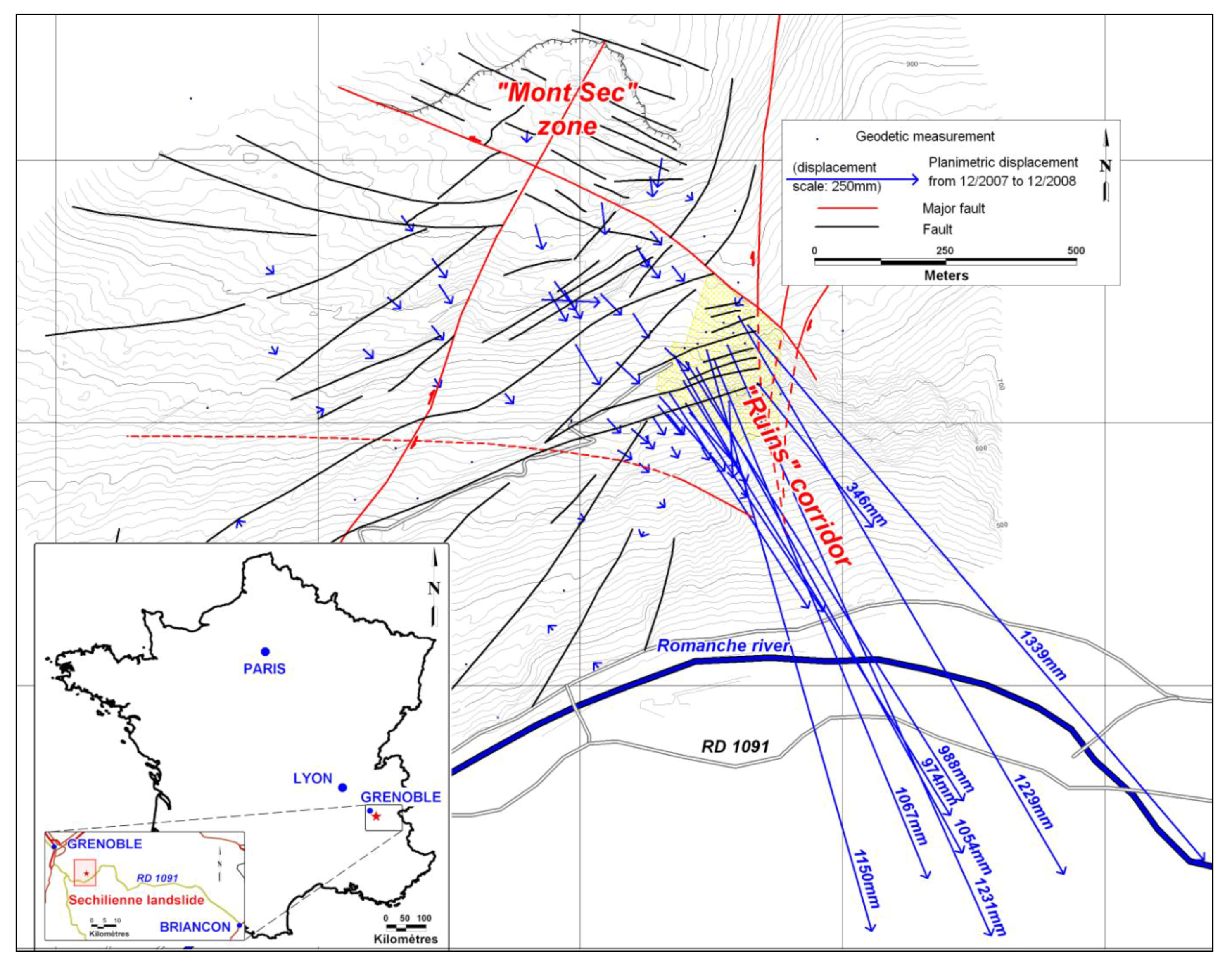
2. The Séchilienne Landslide

Throughout this paper, the case study approach will focus on the Séchilienne landslide located on the north side of the Romanche valley, 20 km southeast of Grenoble (France) in the French Alps (Figure 1). Indeed, during the last centuries, many rockfalls occurred principally from the “Ruines” area, the southern flank of the Mont Sec. In the 1980s, rockfall activity increased and a large slope deformation has been recognized [12]. A massive landslide would cut off a major road, RD1091, which has already been deviated twice. A natural dam could be created across the river causing an upstream lake that, should it break would provoke a catastrophic flood. In 1997, more than 300 people of Montfalcon have been expropriated for risks prevention. More recently, a 39,000 m3 rockfall occurred in November 2006. The monitoring system, initially composed of geodetic and extensometer manual measurements (cables stretched through fractures), was gradually developed and improved.

2.1. Landslide Description

The Séchilienne landslide lies on a SSE facing slope from 600 m above sea level (a.s.l.) up to 1,130 m a.s.l., covering an area of about 70 ha. Between 330 m and 950 m a.s.l., the slope angle is about 40°–50° and it decreases to 20° between 950 m and 1,100 m a.s.l. in the Mont Sec area. On the crest of Mont Sec, a 30 m high scarp, several hundred meters long, caused by the subsidence of the southern part of the hill can be observed (Figure 1). Two main parts have to be considered to describe the landslide: (1) the “Ruines corridor” (RC) (about 3 mil. m3 of rocks), which is the most active part of the landslide; and (2) the upper part of the Mont Sec in subsidence.
The limits of the whole landslide are well defined by a major tectonic shear zone on the eastern border (N20°E: Fault strike directions given clockwise from the north), by the elliptic scarp of Mont Sec in the north, by a stable area at 600 m a.s.l. on the south border, and finally the slope movement gradually decreases in the western part.
Figure 1. Localization of the Séchilienne landslide (Isère, France). Planimetric displacements measured by classical geodetic techniques between December 2007 and December 2008 are blue colored and geological faulting is shown in black and red. The active zone is highlighted in yellow.
Remotesensing 02 02785 g001

2.2. Geological Context

The Séchilienne site is part of the external Belledonne chain, which mainly consists of micaschists [13]: Rocks forming the moving slope belong to an old sedimentary formation made of sandstones and siltic layers named “Série Satinée” [13]. Main schistosity is oriented N20°E with a subvertical dip angle. The landslide area is cut by several faults (Figure 1) and three sets of fractures [13]: Subvertical N20°E as parallel fracture set to the schistosity; subvertical N120°E; and N70°E 80°N. These N70°E 80°N fractures (main set of fractures in the RC area) form slices in the rock mass as shown by uphill facing scarps (up to 100 m long) associated with depressions in that direction.
The deformation process is located within a large and deep-seated movement. It may be described as both toppling and subsidence of vertical rock layers, which are cut across by several discontinuities dating from the Caledonian to Alpine age. Large cracks regularly open in the most active part of the slope meanwhile numerous sinkholes have appeared in the upper part of the Mont Sec area [14,15]. The subsidence of the upper part of Mont Sec, probably initiated thousands years ago after the glacier withdrawal, has accelerated in the active zone of Ruines since the 1980s [15]. But despite all observations made since this landslide has been monitored, no satisfactory explanations have been reported in any study so as to understand the origin of this instability.

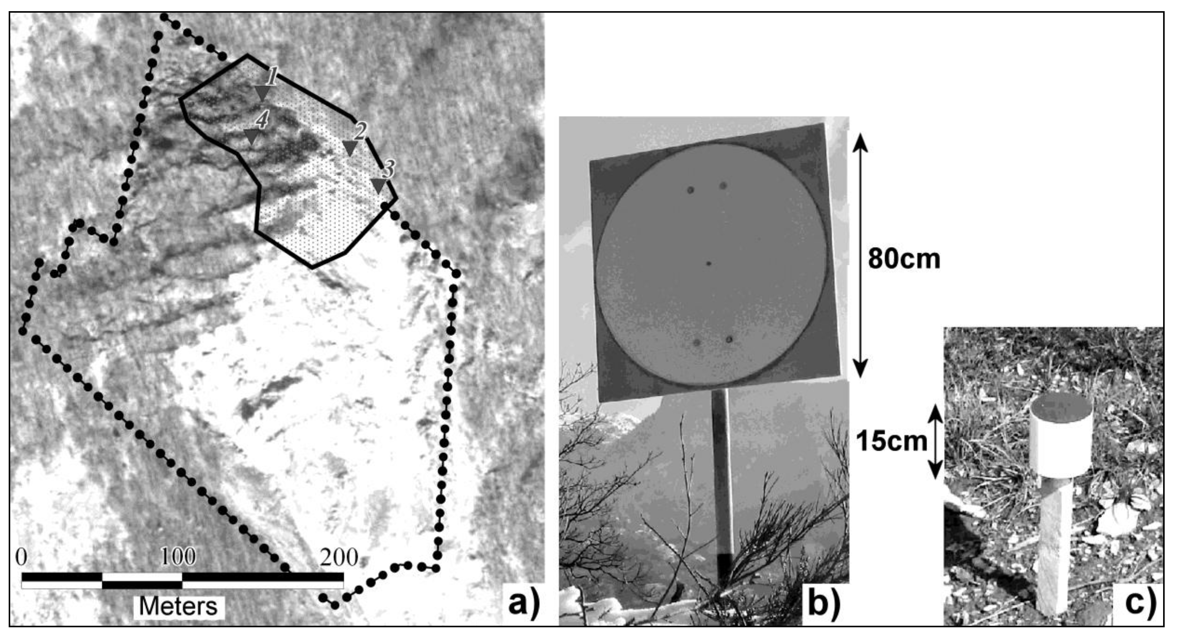
2.3. Landslide Monitoring

The monitoring of the Séchilienne landslide is fully realized by the “Centre d’Etudes Techniques de l’Equipement” (CETE) of Lyon, part of the French ministry in charge of major risk concerns. Since 1985, different field monitoring systems have been deployed to measure displacements: 48 wire extensometric bases, 33 automatic extensometric sensors (placed on the principal fractures), 61 geodetic reflectors and 30 trihedrons. Since 2000, these trihedrons allow an all-weather precise measurement (0.5 ppm) by ground-based radar [17]. Moreover, referenced displacements on the whole southern slope of the Mont Sec (Figure 1) are mapped from an annual geodetic acquisition based on the coordinate measurements of 90 reference marks. The measured displacements on the entire site are globally oriented in a S-SE direction; they are dipping downhill from 10° to 20° in the Mont Sec area up to 45° in the active zone. The displacement rate in this active zone varies on average from 15 cm/yr to almost 160 cm/yr.
Although a lot of monitoring systems are used on the Séchilienne landslide, they cannot provide a full continuous spatial view of displacements, especially in the active zone of the “Ruines corridor”. This study is aimed at testing the applicability of the TLS in the investigation of a large movement and its ability to ensure measurements of displacements in a large disturbed and vegetated zone.
Recently, deep geophysical investigations have been applied to complete surface displacement measurements. Four 950 m long electrical tomography profiles and four 470 m long seismic profiles have been performed on the Séchilienne landslide. The investigations in [18] provide information about depth of unconsolidated rocks (around 130 m in the Mont Sec area and about 90 m in the RC). Knowing these unconsolidated supposed depths, three 150 m long geotechnical boreholes have been drilled to perform inclinometry and piezometry monitoring.

3. Terrestrial Laser Scanner Methodology

3.1. Principle of TLS Acquisitions

Based on the time-of-flight laser measurement technique [19,20,21], TLS allows a 3D point cloud acquisition that would likely turn out to be a technique suited to study complex topographic unstable sites. Thanks to the rotative mirror technology, a laser beam sweeps the surveying surface and is reflected. From the angles of emission and the forward and backward time of the laser pulse, the coordinates of the reflective point of the environment can be inferred. These laser pulses are likely to reflect on topography but also on vegetation and any opaque structure on the laser path. Therefore, to extract the topography, raw data have to be processed. The spatial resolution of the data mainly depends on the angular resolution for pulse emission and the distance between TLS and swept objects. One of the most serious disadvantages of this technique lies in the fact that any object on which the laser pulse is reflected creates a shadow-masked zone behind which there is no data. To overcome this drawback, and so far as possible, several acquisitions from different set-up stations are required. A critical point consists in combining the point clouds acquired from each scan position and transforming the total relative point cloud into absolute spatial coordinates [22]. Then, given the high density of the point cloud (up to 5,000 pts/m2 in our case), high-resolution Digital Elevation Models (DEM) can be provided.

3.2. Characteristics of the RIEGL LMS Z420i

The TLS RIEGL LMS Z420i has been employed to acquire point clouds. This model is essentially characterized by its narrow beam divergence (0.25 mrad), a wide operating range (0° to 80° vertically, 0° to 360° horizontally), and a frequency of about 8,000 points per second. Finally, the measuring range is announced up to 800 m at target with 80% reflectivity. The software RiSCAN PRO has ensured sensor configuration, data acquisition, processing and storage.

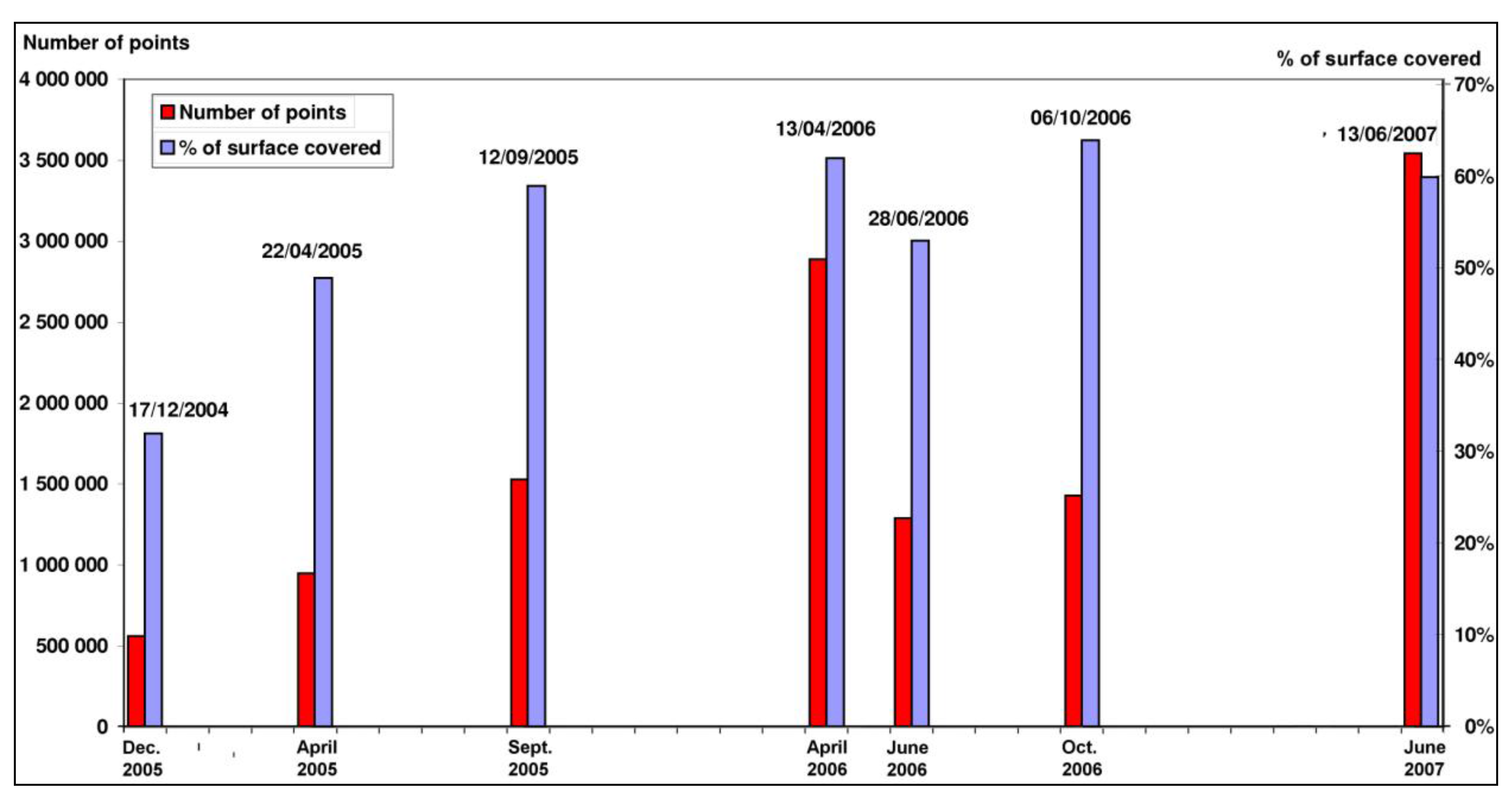
3.3. Acquisition, Registration and Georeferencing

Seven series of measurements were carried out between December 2004 and June 2007 (Figure 2). In the case of the Séchilienne landslide, a scan position on the opposite hillside was inconceivable for the acquisition since the distance (about 1.6 km) exceeded the maximal range of the TLS used. As an alternative, four “on-site” stations along the scarp and on the landslide itself (Figure 3(a)) have been selected in order to limit the shadow-masked zone and enlarge the acquisition area. The TLS distance of acquisition does not exceed 80 m. These four scan positions also ensure a good overlap between the different point clouds acquired from each position, but the surveyed area does not correspond to the entire RC (Figure 3(a)). The scan position located on the top of the eastern cliff (#2 on Figure 3) allows an aerial point of view on the entire zone, whereas data from the other scan positions are discontinuous because of shadow-masked zone (Figure 3(a)), as laser beam impacts the topography almost tangentially.
The positions of thirty-two retro-reflective targets laid in the environment (30 cylinders located in the landslide (Figure 3(c)) and two discs out of the active zone (Figure 3(b)) have been measured by standard topographical techniques with a total station. These targets enable merging the four scans acquired from each scan position [13] and to georeference the total point cloud.
The Iterative Closest Point (ICP) algorithm [23], which is a classic mean of registration of TLS point clouds is generally applied. In our case, significant surface changes have occurred between the different scan surveys. The surfaces, being unalike, reduce the reliability of matching making ICP not well suited to this application.
Figure 2. Date of acquisition, number of points covered by the TLS acquisitions, and percentage of surface covered.
Remotesensing 02 02785 g002
Figure 3. Localization of the TLS view points on the RC area (dashed line) and area covered by TLS point clouds (solid line) (a); big (b) and small (c) retro-reflective targets used to ensure georeferencing and merging scans from the different points of view.
Remotesensing 02 02785 g003

3.4. Post Processing and TLS Accuracy

In addition to the gaps caused by shadow-masked zones, the point clouds density is heterogeneous because of distances and angles of incidence of laser beam on the reflective surface. For practical purposes, before creating DEMs, post-processing is carried out by TerraScan algorithms to extract only the back-scattered pulses due to the topography. Density calculations and raster DEMs have been computed thanks to codes written in Interactive Data Language (IDL): Density is obtained by counting the corresponding number of scanned points for each pixel and DEMs computation uses bilinear interpolation.
Considering the sliding velocity previously measured by standard topographical techniques, the landslide is expected to carry large amounts of material away between two successive measurements. Therefore, as it was obvious that the TLS accuracy would be sufficient to detect changes, no further investigation of the laser data accuracy has been performed, apart from a test on a natural target on the Séchilienne landslide. The single point accuracy announced for this TLS is 10 mm at 50 m. Given the results of the test, a +/−15 mm difference has to be considered on the three axis for a distance of acquisition of 80m, which is the maximal distance in this study. This test gives an estimation of the accuracy comparing overlapping points acquired from different scan positions. TLS dataset accuracy and DEM subtraction accuracy can vary because of two main reasons: (1) The interpolation made to rasterize TLS dataset clearly damages the quality of the data and reduces the original accuracy of TLS datasets; (2) the accuracy of topography on stable areas used for comparison. In our case, the accuracy of DEM subtraction is actually evaluated by the error on the stable east-bordering cliff (Figure 4). The problem is that the stable part is grassy. And yet, the height of the grass has an influence on what is considered as topography by the TerraScan filtering algorithm. Thus, accuracy of DEMs subtraction is evaluated at 250 mm. The actual accuracy of object recognition on transects analysis has been carried out on the vertical part of the east border cliff. This cliff is grass-free, allowing estimations of accuracy in three directions on a small scale. Thus, an accuracy of 30 mm has to be considered in the X, Y, and Z directions, for object recognition on transects analysis. Accuracy estimation is different if based on rocks or grassy area.
Figure 4. Differences between real displacements and observed displacements when considering DEM subtractions.
Remotesensing 02 02785 g004

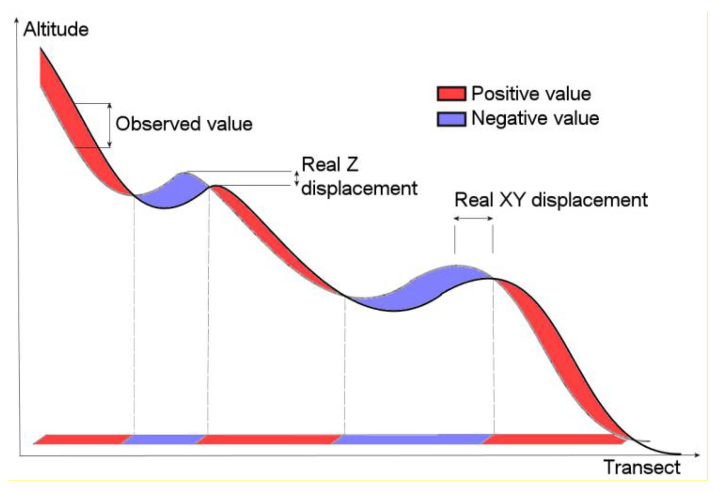
3.5. Displacement Characterization and Quantification

Point cloud data can be analyzed in various ways, such as point to point comparison [11,12], or DEM comparisons [3,10,24]. A quantification of displacements based on objects recognition in transects analysis can also be achieved. In the case of the Séchilienne landslide, occlusions prevent us from performing a 3D analysis and has been replaced by DEM comparisons and transects analysis. Indeed, object recognition has been applied in order to characterize displacements with an important horizontal component even when numerous points are missing due to occlusions. 2-D transects have been performed in the main direction of movement (N150°E).
Twenty centimeters cell-size DEMs are generated for each acquisition. Because of the occlusions, DEMs cannot be directly compared. Effective acquired points cannot be distinguished from interpolated points. Discontinuous masks, representing effective presence of acquired points (at least one point per DEM cell of 400 cm2), have been applied on the DEMs: Shadow areas were no longer taken in account. This point makes the interpretation of the DEM subtractions difficult as it prevents a continuous visualization of the results.

4. Results and Interpretations

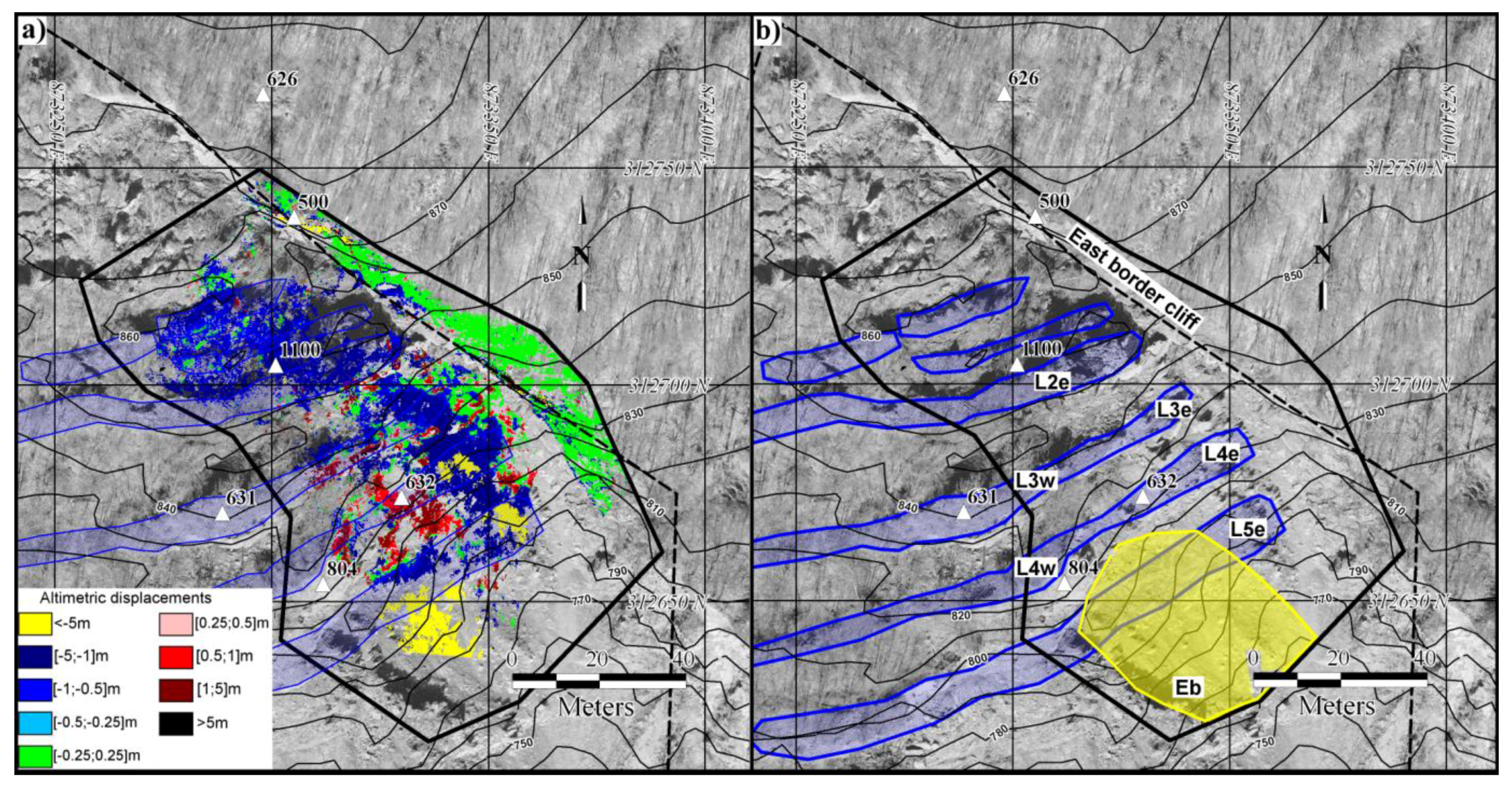
4.1. DEMs Subtractions

DEMs subtractions allow quantifying the variations of topography: A negative value on Z‑coordinates corresponds to subsidence or ablation of rocks; whereas positive values point out a movement where subsidence is combined with the landslide advancing (due to the combination of horizontal and vertical displacements (Figure 4)).
Rockfall detection and quantification can be achieved (Figure 5(a), Figure 6 and Figure 7). Results of the DEM subtractions are mapped on an ortho-image (Figure 5(a)) to make the localization of the different areas within the RC easier (Figure 5(b)). Different collapses are highlighted (Eb, L4e and L5e).
A first collapse occurred in the Eb zone between April and September 2005 (Figure 5 and Figure 7) that removed about 1 m of surface rocks. The northern part of this zone then subsided 10 to 12 cm/month between September 2005 and October 2006 before the main collapse in November 2006. N70°E sliced structures consist of soft materials between massive and inured rocks that have a low fracturing level (Figure 6). These materials are made up of quaternary infillings and debris from precedent movements. The eastern parts of these structures are about 15 m high for L4e and 5 m high for L3e and L5e. L3e and L5e disappeared between April and September 2005. The western parts of these structures (L3w, L4w and L5w) show the same subsidence.
One major drawback of this approach is that the DEM subtraction method is insufficient to completely characterize displacements, especially when DEM is incomplete because of occlusions. On the other hand, the method using 2D transects gives information on real displacements in this active zone with better results.
Figure 5. Altimetric variations between September 2005 and June 2007 mapped on an ortho-image. Altimetric displacements are based on the TLS acquisition zone: Rockfalls of L4e, L5e and Eb are yellow colored and the east border cliff appears stable. (a) Locations of the N70°E structures (blue colored) and limits of the November 2006 collapse (Eb) in the active zone; (b) RC is dashed delimited, area monitored by TLS is black color delimited. Western and eastern part of each N70°E structure in RC are distinguished (respectively L4w and L4e).
Remotesensing 02 02785 g005
Figure 6. Photograph of the L4e structure which collapsed in May 2005, taken from an eastern point of view of the N70°E structures in the RC zone.
Remotesensing 02 02785 g006
Figure 7. DEM subtractions in December 2004, April 2005, September 2005, April 2006, October 2006 and June 2007, mapped on an ortho-image. N70°E structures are blue contoured.
Remotesensing 02 02785 g007

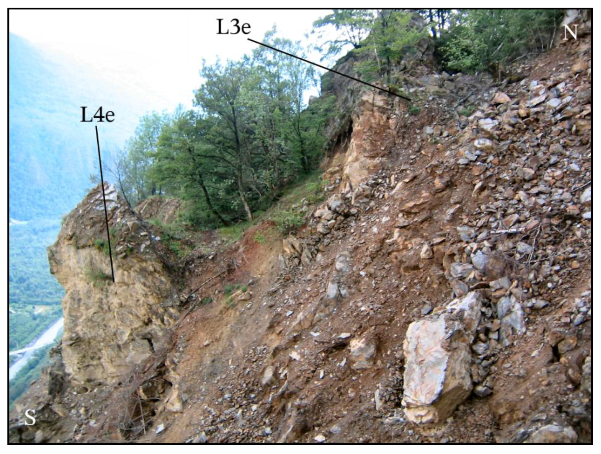
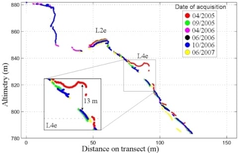
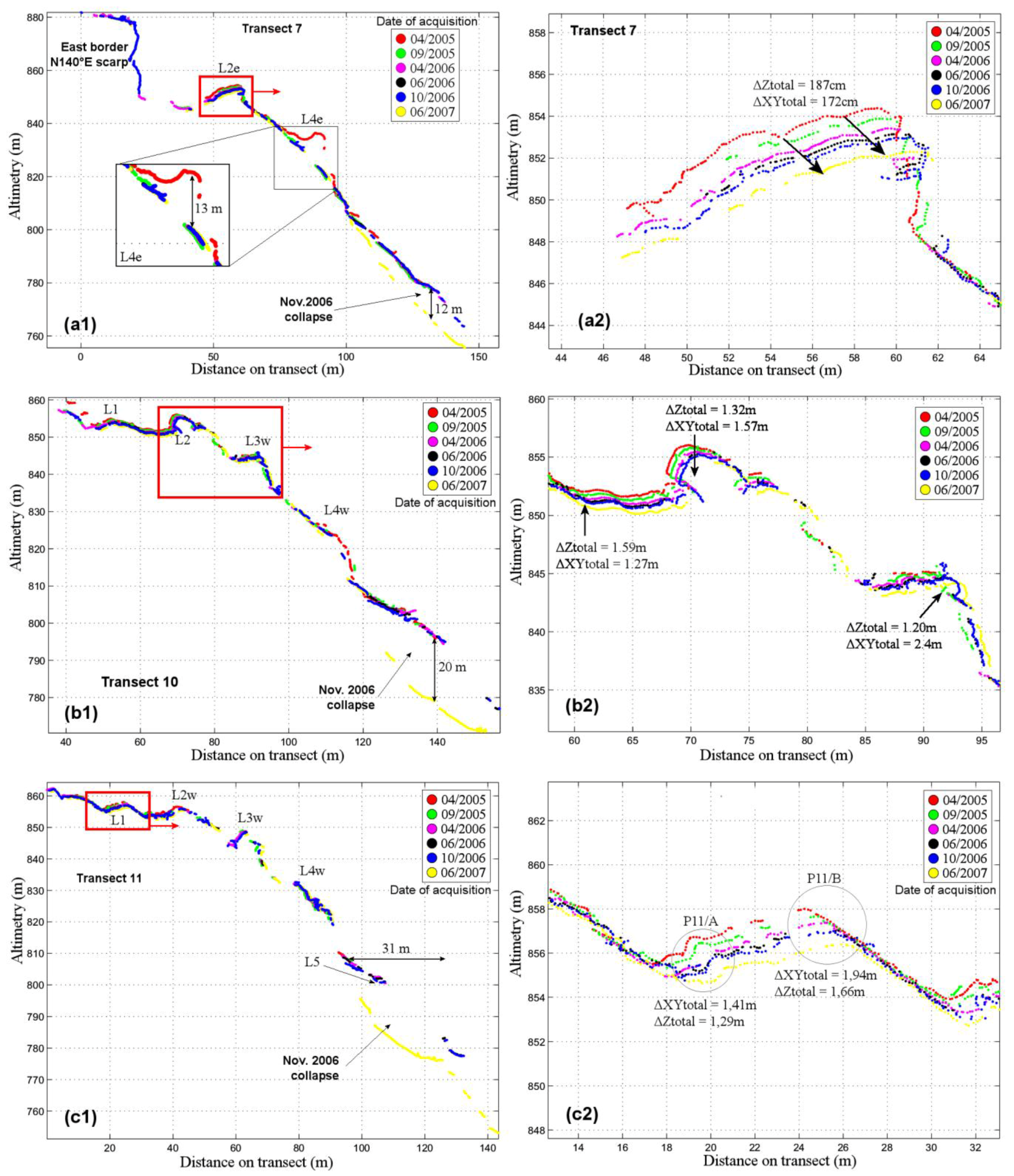
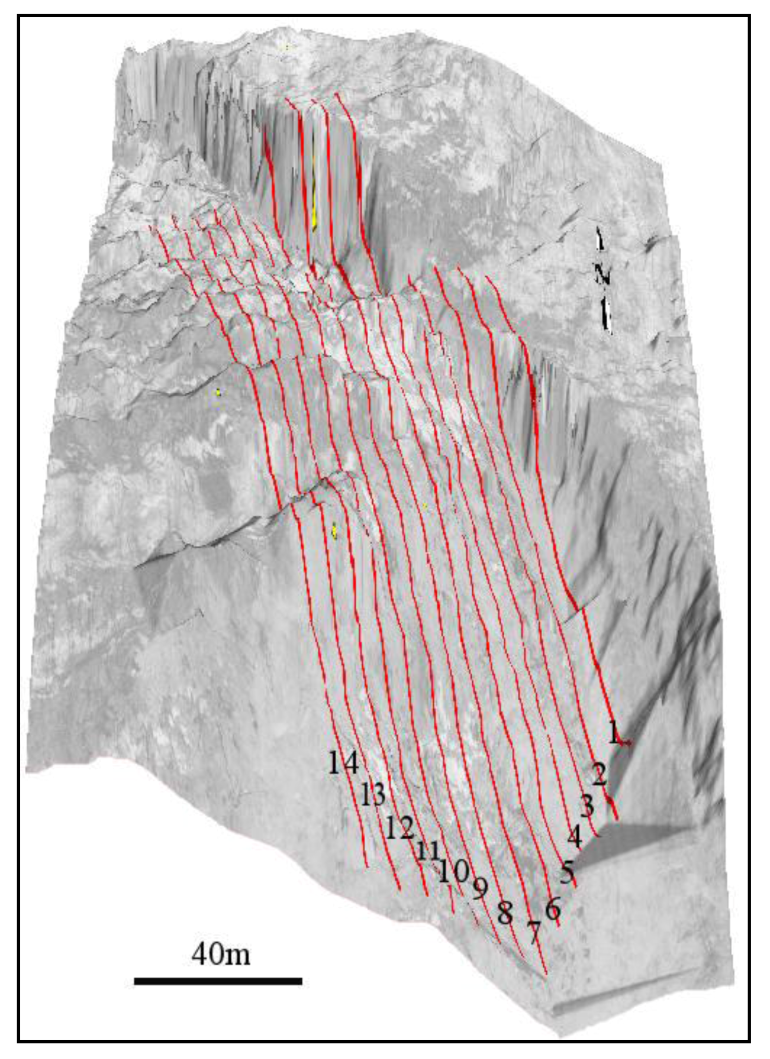
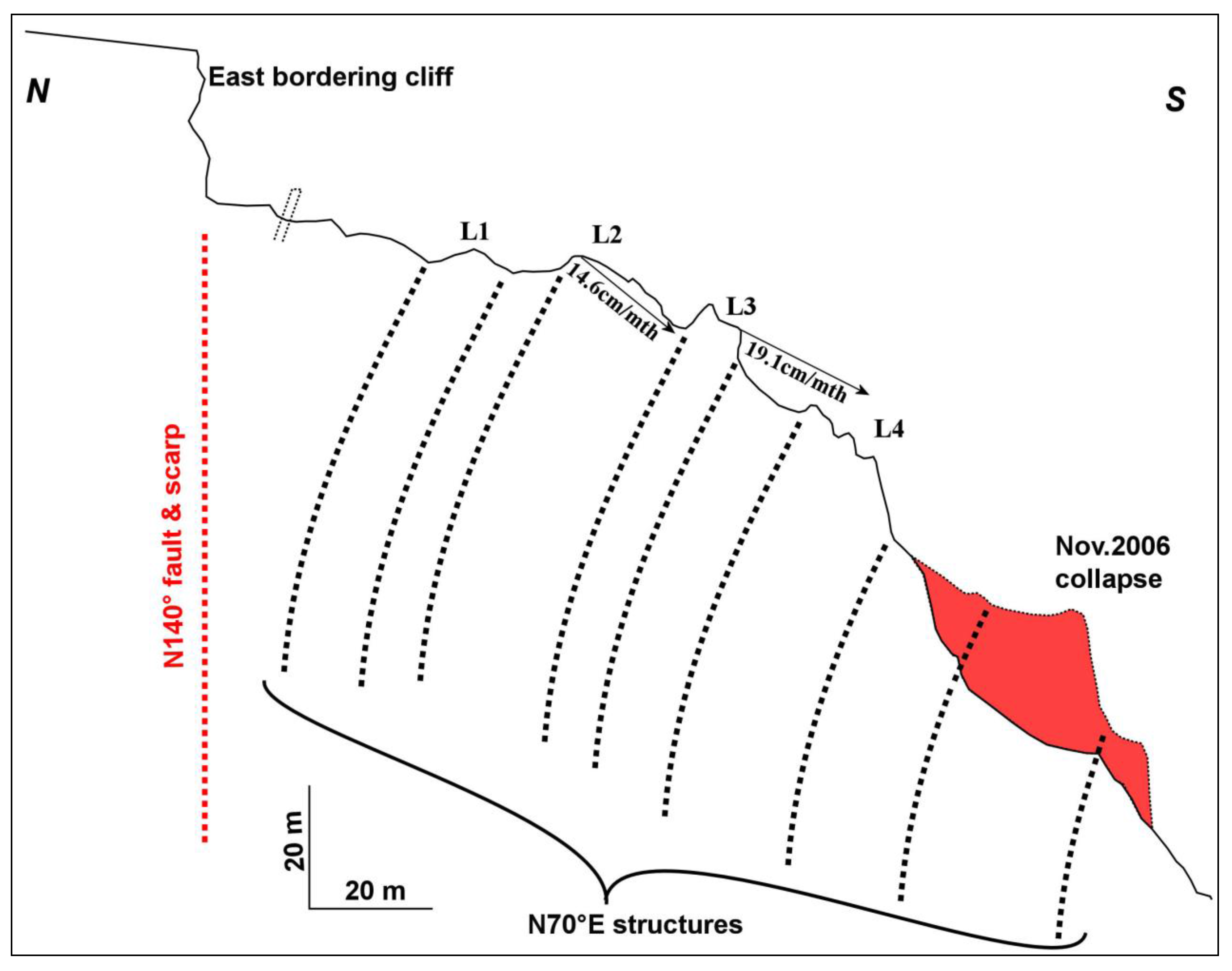
4.2. Displacement Measurements on Transects

The point clouds are dense enough (at least one point every 10 cm) to build transects and to process them without any interpolation, even if occlusions did not allow sampling over the whole profile length. Once the point clouds are georeferenced, transects can be defined in all directions. A N150°E direction has been chosen to follow the main direction of movement (Figure 8). Only points located +/−10 cm from the transect lines are allowed in the data for profiles.
Figure 8. Localization of transects realized in TLS data, represented in 3D.
Remotesensing 02 02785 g008
The examination of the transects (Figure 9) confirms that the whole zone of Ruines is moving and that no stable zones are observed apart from the east bordering cliff. Even if occlusions prevent computing a point to point volume estimation, the geometrical parameters of the L4e collapse (before September 2005) and the November 2006 Eb collapse, can be specified: The L4e N70°E structure is 13 m high and approximately 10 m wide (Figure 9(a1)). The volume is about 1,250 m3 collapsed volume. With regard to the November 2006 Eb collapse (Figure 9(a1,b1,c1), an approximate calculation with a truncated pyramid of 15m high, a 75 × 50 m base and a 40 × 40 m summit face, leads to an estimation of the collapsed volume of about 39,000 m3.
Considering the data from April 2005 to June 2007, all the various N70°E structures show the same movements but at various speeds i.e. depressions in the upper part that extend to the main bodies. The L2 structure shows various fields of speed according to N150°E transects: The eastern part of the #7 transect (Figure 9(a2)) has a global movement of 2.54 m (subsidence of 187 cm and horizontal displacement of 172 cm) with an apparent plunging angle of 47°. In the western part, on transect number 10 (Figure 9(b2)), the same N70°E structure has an apparent plunging of 40° for only 2.05 m of global amplitude (subsidence of 132 cm and horizontal displacement of 157 cm).
Figure 9. N150°E transects in TLS data (#7, #10 and #11). N70°E structures clearly show movement with a 42° global dip and a mean of 7 to 10 cm per month. Collapses of these structures are specified.
Remotesensing 02 02785 g009
The depletion zones separating the N70°E structures are more affected by subsidence than the structures themselves, with a 159 cm displacement in depletion zones between L1 and L2, compared to 132 cm on top of the L2 structure (Figure 9(b2)). In comparison with L2, the L3w structure shows a more marked horizontal displacement of 2.4 m for a subsidence of 1.2 m (apparent plunging of only 27°) (Figure 9(b2)). Its global displacement is 2.68 m during the considered period (from April 2005 to June 2007). The L1 structure emphasizes the differences between northern and southern parts (respectively P11_A and P11_B on Figure 9(c2)) of the same structure: While preserving the same vertical direction (apparent plunging of 40°), southern zone displacements are 30% higher than the upstream northern part, highlighting the toppling part of the displacements. In that direction (N150°E), and on the surface of the L1 structure, toppling can be estimated as 5° between April 2005 and June 2007.
Considering the L1 displacements, it seems that the mass moved down-slope according to a constant apparent plunge of 40°. Although this could be connected with a sliding surface, none of the collected geological information confirms such a plane. It is rather likely that the hardened zones delimited by the N70°E structures adapt this constant displacement by operating a toppling combined with a subsidence. As all TLS were carried out with excellent covertures of the L1 structure, evolution of the RC zone during a period without available data (Table 1) can still be assumed in the P11_A and P11_B areas (Figure 9(c2)). Two outstanding points emerge from the data: Firstly, the amplitude of movement decreases on the P11_A and P11_B zones from 10 to 12 cm per month between April 2005 and June 2006 to 6 to 7 cm per month between June 2006 and June 2007 (Table 1). This has been corroborated by geodetic measurements of the monitoring system (targets 1,100, 804 and 631, Table 2). Secondly, plunging angles of displacements have also changed: From about 30° between October 2006 and April 2006, and after April 2006 they are about 50°–65° (Table 1). The difference between geodetic measurements and TLS data is about 10° in the plunging angle (Table 2). This difference can be explained by the fact that measures on the TLS point clouds are realized by form recognition. In any case, April 2006 marks the beginning of a new stage of evolution in the RC zone, but there is still no reliable explanation.
Table 1. Evolution of the two parts (P11_A and P11_B, transect #11) of the N70°E structure. Notice that dip angles of both parts change in April 2006.
P11_A
DatesδXY (+/−4.24 cm)δZ (+/−3 cm)DipAmplitude (+/−4.24 cm)Amplitude (+/−0.4 cm/mth)
04/2005–09/200536−2333°(+/−6°)439
09/2005–04/200644−2328°(+/−5°)507
04/2006–06/200619−26,554°(+/−9°)3311
06/2006–10/200610−11,850°(+/−19°)155
10/2006–06/200732−41,152°(+/−6°)527
04/200506/200714112942°(+/2°)1917
P11_B
DatesδXY (+/−4.24 cm)δZ (+/−3 cm)DipAmplitude (+/−4.24 cm)Amplitude (+/−0.4 cm/mth)
04/2005–09/200559−3631°(+/−4°)6914
09/2005–04/200672−31,724°(+/−3°)7911
04/2006–06/200623,9−30,652°(+/−8°)3913
06/2006–10/200614,7−17,350°(+/−13°)238
10/2006–06/200723,1−4965°(+/−5°)547
04/200506/200719416641°(+/1°)25510
Table 2. Evolution of geodetic targets from November 2004 to November 2005.
TargetPeriod between 11/2004 and 11/2005Period between 11/2005 and 11/2006
δXYZ (cm)δXYZ (cm/month)DirectionDipδXYZ (cm)δXYZ (cm/month)DirectionDip
63112510.4151°30°111.29.2151°30°
11001129.3150°36°102.18.5151°37°
834836.9150°30°77.66.4151°28°

4.3. Interpretation and Instability Considerations

Previous studies were based on classical topographic measurements and morphological information. Evolutions of the N70°E structures were identified as the main factor of instability in RC. Incidentally, numerical models with northern dip for N70°E structures have been developed [13,25] explaining depressions between N70°E structures. With TLS acquisitions, it is the first time that the evolution of each N70°E structure in RC can be described.
By fieldworks, some holes and cracks were noticed between each N70°E structure, but they do not appear on the TLS dataset. These holes are not clearly detected because rocks surrounding them are constantly rearranged. The signature of these holes mainly consist of depression between each N70°E structure (Figure 10). Indeed, main back-cracks were observed in the north and north-west, outside the area in which data has been TLS acquired (Figure 2(a)). Results from TLS data sets mainly refer to inner RC observations.
Concerning movements, N70°E structures combine subsidence, translational and rotational displacements. The entire RC area is moving down in a N150°E direction which is almost perpendicular to these massive N70°E structures. According to previous models developed [13], a first order conceptual interpretation (Figure 10) can be drawn from the measurements of surface displacements and the main geological setting of the N70°E structures in the RC zone. Without clear information about their dip angle, N70°E structures are presumed to have a northern dip cut varying with depth.
Considering: (1) Holes are created between each N70°E structure; (2) the high internal deformation of rockmass should reach 90 m in depth [18]; and (3) collapses observed show that, currently and in the past, only small volumes are concerned; we hypothesize a ‘toppling like’ mechanism controlled by the N70°E structures explaining the dip variation with depth. Such a mechanism could explain the observed displacements occurring without main collapses.
Figure 10. Interpretation of mechanisms deduced from TLS data on a N150° cross section. The November 2006 collapse is underlined in red. Movements are limited by the N140°E east bordering cliff.
Remotesensing 02 02785 g010

5. Conclusions and Perspectives

From the sequential TLS datasets, DEMs subtractions, with an accuracy of 250 mm, have allowed us to spatially determine the moving zones. The most important limitation of this method lies in the fact that it only gives information about altitude changes. Nevertheless, object recognition based on 2D transects in the main direction of displacements, can complete the information enabling quantification of displacements with a precision of +/−30 mm in all directions. The current study was limited by the position of accessible points of view; nevertheless, TLS proved to be a very suitable tool as it provides high resolute point clouds of the topography. As they were not completely frontal, some point clouds have suffered from shaded areas created by vegetation and chaotic zones. This problem prevents a full spatially covered analysis. In such cases, aerial laser scanning by helicopter would give better coverage as it would provide data both in cliff areas and holes hidden by the chaotic topography, but with less resolution and accuracy.
The results of the analysis of the 2D transects realized through TLS point clouds, showed the subsidence, the translation, and the toppling of the N70°E structures, which affect the Ruines zone. By supplying the entire topographical evolution of the N70°E structures, TLS acquisitions confirm previous models: Indeed, it seems that rotations of these structures could explain displacements such as a huge toppling. Further work, especially in depth studies, needs to be done to explain this instability. In this direction, two inclinometers have been installed in 2009 and 2010 in order to provide such data.

Acknowledgments

This work has been partially funded by the EU-Research Project ClimChAlp (Climate Change, Impacts and Adaptation Strategies in the AlpineSpace). Monitoring data from the Séchilienne landslide is entirely covered by the monitoring section of the Rock Mechanics Division of the CETE de Lyon: Authors gratefully thank them for their help. Moreover authors thank the three anonymous reviewers whose comments substantially helped to improve the paper.

References and Notes

  1. Angeli, M.C.; Pasuto, A.; Silvano, S. A critical review of landslide monitoring experiences. Eng. Geol. 2000, 55, 133–147. [Google Scholar] [CrossRef]
  2. Squarzoni, C.; Delacourt, C.; Allemand, P. Differential single-frequency GPS monitoring of the La Valette landslide (French Alps). Eng. Geol. 2005, 79, 215–229. [Google Scholar] [CrossRef]
  3. Bitelli, G.; Dubbini, M.; Zanutta, A. Terrestrial laser scanning and digital photogrammetry techniques to monitor landslide bodies. In International Archives of the Photogrammetry, Remote Sensing and Spatial Information Sciences; In Proceedings of the XXth ISPRS Congress: Geo-Imagery Bridging Continents, Istanbul, Turkey, July 12–23, 2004; Volume XXXV, Part 5. pp. 246–251.
  4. Delacourt, C.; Allemand, P.; Berthier, E.; Raucoules, D.; Casson, B.; Grandjean, P.; Pambrun, C.; Varrel, E. Remote-sensing techniques for analysing landslide kinematics: A review. Bull. Soc. Géolog. France 2007, 178, 89–100. [Google Scholar] [CrossRef]
  5. Oppikofer, T.; Jaboyedoff, M.; Keusen, H.-R. Collapse at the eastern Eiger flank in the Swiss Alps. Nature Geosci. 2008, 1, 531–535. [Google Scholar] [CrossRef]
  6. Oppikofer, T.; Jaboyedoff, M.; Blikra, L.; Derron, M.-H.; Metzer, R. Characterization and monitoring of the Åknes rockslide using terrestrial laser scanning. Nat. Hazards Earth Syst. Sci. 2009, 9, 1003–1019. [Google Scholar] [CrossRef]
  7. Teza, G.; Galgaro, A.; Zaltron, N.; Genevois, R. Terrestrial laser scanner to detect landslide displacement fields: a new approach. Int. J. Remote Sens. 2007, 28, 3425–3446. [Google Scholar] [CrossRef]
  8. Abellán, A.; Jaboyedoff, M.; Oppikofer, T.; Vilaplana, J.M. Detection of millimetric deformation using a terrestrial laser scanner: Experiment and application to a rockfall event. Nat. Hazards Earth Syst. Sci. 2009, 9, 365–372. [Google Scholar] [CrossRef]
  9. Travelletti, J.; Oppikofer, T.; Delacourt, C.; Malet, J.-P.; Jaboyedoff, M. Monitoring landslide displacements during a controlled rain experiment using a long-range terrestrial laser scanning (TLS). In International Archives of the Photogrammetry, Remote Sensing and Spatial Information Sciences; In Proceedings of XXIst ISPRS Congress: Commission V, WG 3, Beijing, China, July 3–11, 2008; Volume 37, Part B5. pp. 485–490.
  10. Abellán, A.; Vilaplana, J. M.; Martínez, J. Application of a long-range terrestrial laser scanner to a detailed rockfall study at Vall de Núria (Eastern Pyrenees, Spain). Eng. Geol. 2006, 88, 136–148. [Google Scholar] [CrossRef]
  11. Bauer, A.; Paar, G.; Kaltenbock, A. Mass movement monitoring using Terrestrial Laser Scanner for rock fall management. In Geo-information for Disaster Management; Van Oosterom, P., Zlatanova, S., Fendel, E.M., Eds.; Springer: Berlin, Germany, 2005; pp. 393–406. [Google Scholar]
  12. Antoine, P.; Camporota, P.; Giraud, A.; Rochet, L. La menace d’écroulement aux Ruines de Séchilienne (Isère). Bulletin des laboratoires des Ponts et Chaussées 1987, 150/151, 55–64. [Google Scholar]
  13. Pothérat, P.; Alfonsi, P. Les mouvements de Séchilienne (Isère)—Prise en compte de l'héritage structural pour leur simulation numérique. Revue française de géotechnique 2001, 95/96, 117–131. [Google Scholar]
  14. Alfonsi, P. Relation entre les paramètres hydrologiques et la vitesse dans les glissements de terrains. Exemple de la Clapière et de Séchilienne (France). Revue française de géotechnique 1997, 79, 3–12. [Google Scholar]
  15. Durville, J.-L.; Effendiantz, L.; Pothérat, P.; Marchesini, P. The Séchilienne landslide. In Identification and Mitigation of Large Landslide Risks in Europe: Advances in Risk Assessment; Bonnard, C., Forlati, F., Scavia, C., Eds.;IMIRILAND Project: European Commission—Fifth Framework Program; A.A. Balkema Publishers: London, UK, 2004; pp. 253–269.
  16. Leroux, O.; Schwartz, S.; Gamond, J.-F.; Jongmans, D.; Bourles, D.; Braucher, R.; Mahaney, W.; Carcaillet, J.; Leanni, L. CRE dating on the head scarp of a major landslide (Séchilienne, French Alps), age constraints on Holocene kinematics. Earth Planet. Sci. Lett. 2009, 280, 236–245. [Google Scholar] [CrossRef]
  17. Duranthon, J.-P.; Effendiantz, L. Le versant instable des “Ruines” de Séchilienne. Point sur l’activité du phénomène et présentation du nouveau dispositif de gestion de la télésurveillance. Bulletin des laboratoires des Ponts et Chaussées 2004, 252/253, 29–48. [Google Scholar]
  18. Kasperski, J.; Jongmans, D.; Lagabrielle, R.; Pothérat, P.; Méric, O. Apport des reconnaissances profondes par méthodes géophysiques sur le mouvement de versant de Séchilienne (Isère). In Proceedings of Rock Slope Stability, Paris, France, November 24–25, 2010.
  19. Baltsavias, E. Airborne laser scanning: basic relations and formulas. ISPRS J. Photogramm. Remote Sens. 1999, 54, 199–214. [Google Scholar] [CrossRef]
  20. Lichti, D.D.; Gordon, S.J.; Stewart, M.P. Ground-based laser scanners: Operation, systems and applications. Geomatica 2002, 56, 21–33. [Google Scholar]
  21. Slob, S.; Hack, R. 3-D Terrestrial Laser Scanning as a New Field Measurement and Monitoring Technique. In Engineering Geology for Infrastructure Planning in Europe. A European Perspective; Lecture Notes in Earth Sciences; Hack, R., Azzam, R., Charlier, R., Eds.; Springer: Berlin/Heidelberg, Germany, 2004; Volume 104, pp. 179–190. [Google Scholar]
  22. Riegl, J.; Studnicka, N.; Ullrich, A. Merging and processing of laser scan data and high-resolution digital images acquired with a hybrid 3D laser sensor. In Proceedings of CIPA, XIXth International Symposium, Antalya, Turkey, 30 September–4 October, 2003.
  23. Besl, P.; McKay, N. A method for registration of 3-d shapes. IEEE Trans. Pat. Anal. Mach. Intel. 1992, 14, 239–256. [Google Scholar] [CrossRef]
  24. Prokop, A.; Panholzer, H. Assessing the capability of terrestrial scanning for monitoring slow moving landslides. Nat. Hazards Earth Syst. Sci. 2009, 9, 1921–1928. [Google Scholar] [CrossRef]
  25. Vengeon, J.-M.; Giraud, A.; Antoine, P.; Rochet, L. Contribution à l’analyse de la déformation et de la rupture des grands versants rocheux en terrain cristallophyllien. Can. Geotech. J. 1999, 26, 1123–1136. [Google Scholar] [CrossRef]

