
Research on UWB Indoor Positioning Algorithm under the Influence of Human Occlusion and Spatial NLOS


School of Instrument Science and Engineering, Southeast University, Nanjing 210096, China
*
Author to whom correspondence should be addressed.
Remote Sens. 2022, 14(24), 6338; https://doi.org/10.3390/rs14246338
Submission received: 9 November 2022
/
Revised: 11 December 2022
/
Accepted: 12 December 2022
/
Published: 14 December 2022
(This article belongs to the Special Issue Advanced Technologies for Position and Navigation under GNSS Signal Challenging or Denied Environments II)
Abstract
:Ultra-wideband (UWB) time-of-flight (TOF)-based ranging information in a non-line-of-sight (NLOS) environment can display significant forward errors, which directly affect positioning performance. NLOS has been a major factor limiting the improvement of UWB positioning accuracy and its application in complex scenarios. Therefore, in order to weaken the influence of the indoor complex environment on the NLOS environment of UWB and to further improve the performance of positioning, in this paper, we first analyze the factors and characteristics of NLOS formation in an indoor environment. The NLOS is divided into fixed NLOS influenced by spatial structure and dynamic random NLOS influenced by human occlusion. Then, the anchor LOS/NLOS information map is established by making full use of indoor spatial a priori information. On this basis, a robust adaptive extended Kalman filtering algorithm based on the anchor LOS/NLOS information map is designed, which is not only effectively able to exclude the influence of spatial NLOS, but can also optimize the random error. The proposed algorithm was validated in different experimental scenarios. The experimental results show that the positioning accuracy is better than 0.32 m in complex indoor NLOS environments.
1. Introduction
With the advancement of technology and the demand for location-based services (LBS), positioning technology has made a qualitative leap in terms of technology, positioning accuracy, and availability. In the outdoors, the global navigation satellite system (GNSS) has achieved great success in positioning in open outdoor areas and has largely met the demand for location-based services in outdoor scenarios through a variety of complementary technologies [1]. However, in an indoor environment, where the majority of human daily activities take place [2], GNSS signals are severely attenuated due to spatial occlusion, making it impossible for GNSS to provide continuous and reliable positioning, especially in deeper inner areas where a GNSS signal may be completely blocked [3]. Therefore, a positioning technology that is suitable for inner environments has been the focus of widespread research, and thanks to the continuous development and popularity of electronic manufacturing processes and communication technologies, a variety of methods and techniques for indoor positioning have emerged [4,5,6,7,8,9,10]. Compared with other radio frequency (RF) positioning technologies, UWB is the preferred solution for high accuracy indoor positioning due to its nanosecond non-sinusoidal narrow pulse characteristics and high-speed data transmission, which can achieve centimeter-level ranging accuracy, as well as its penetration, low power consumption and strong anti-interference capabilities [11]. However, in the face of complex spatial structures and variable spatial environments, UWB and other RF signals are subject to NLOS, multipath effects and other factors, which increase the signal flight time and can lead to serious errors in the ranging values, directly affecting UWB positioning accuracy. Many scholars have provided their insights on the research of NLOS error suppression. Chen investigated the adaptive mitigation through the use and optimization of machine learning models, including deep neural networks (DNN), convolutional neural networks (CNN) and long short-term memory (LSTM). Using the proposed circularly polarized antenna combined with the optimized LSTM model, a three-anchor UWB system for autonomous vehicle localization in severe NLOS environments was built for a 45 m2 area [12], where Li proposed a factor graph-based UWB localization algorithm based on improved Turkey robust kernel. For UWB data, which are generally larger than their true value due to barriers, a robust kernel was added to the simple large ranging data and the square of the residuals was used as the objective function for optimization [13]. Cao proposed a new localization strategy combining calibration, a variational Bayesian unscented Kalman filter (VBUKF), total least squares (TLS) and a water cycle algorithm (WCA) in order to improve the localization accuracy of UWB localization systems in complex subsurface environments [14]. Liu proposed a method for tracking errors of variables such as position, velocity and orientation using a complementary Kalman filter (CKF) to fuse and filter UWB and IMU (inertial measurement unit) data [15].
In general, improving the positioning accuracy of the system by efficiently identifying and eliminating NLOS errors has been the focus of research, but the use of a priori information on the structure of interior spaces is still lacking. Aiming at complex structure in interior spaces and the interference of random human flow in the environment, in this paper, a localization method with antidifference adaptive extended Kalman filtering based on the anchor LOS/NLOS information map is proposed. The main contributions of our research are as follows:
- Firstly, the main characteristics of NLOS in an indoor environment are analyzed. The NLOS is divided into static NLOS influenced by spatial structure and dynamic NLOS generated by the random occlusion of the human body.
- Secondly, using the indoor spatial structure relationship and combining it with the deployment location of anchors, we can quickly and easily establish anchor LOS/NLOS information mapping and accurately distinguish LOS/NLOS anchors.
- Finally, the established LOS/NLOS information map anchors are combined with adaptive antidifference filtering to perform the online preferential positioning of anchors and measure the degree of anomalies of measured values. Furthermore, an adaptive extended Kalman filtering algorithm based on an LOS/NLOS information map is designed and the system performance is verified.
The remainder of this paper is organized as follows: Section 2.1 analyzes the ranging error characteristics of UWB in different NLOS environments and proposes a solution. Section 2.2 designs the method for the fast establishment of an LOS/NLOS information map for indoor anchors. Section 2.3 describes the localization solution algorithm for UWB. Additionally, Section 2.3.3 depicts the design of a localization algorithm based on the anchor LOS/NLOS information map to solve the NLOS occlusion effect of indoor building structures. The improved algorithm that can optimize both spatial NLOS occlusion effects and dynamic human occlusion effects is described in detail in Section 2.3.4. The detailed experimental setup and discussions are reported and analyzed in Section 3. Finally, Section 4 summarizes the work by drawing several conclusions and provides an outlook for future research.
2. Methodology
2.1. NLOS Effect Analysis of UWB Ranging
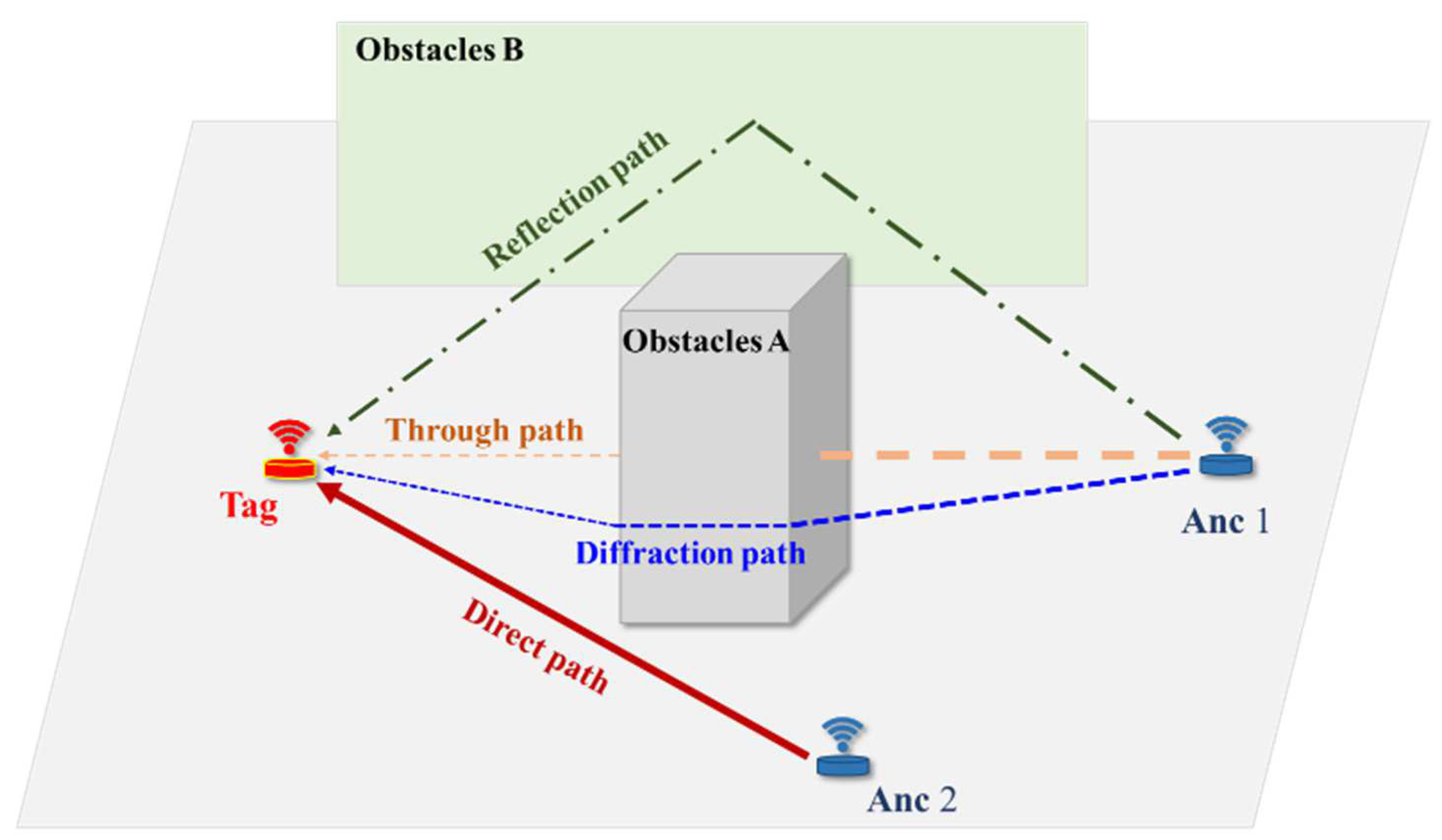
The ranging accuracy of UWB depends mainly on the accuracy of the signal time of flight (TOF). In an LOS environment, since there is no occlusion between the transceiver devices, the direct signal has the shortest distance and requires the least energy attenuation compared to the multipath signal, and the UWB has high ranging accuracy due to its own nanosecond narrow pulse characteristics. In an NLOS situation, the signal propagation path is more complex, as shown in Figure 1 for the anchor (Anc 1), and the direct path is blocked by spatial obstacles; the signal propagation path changes to transmission, reflection and diffraction, and the change of propagation medium or path causes the TOF ranging values to generate different degrees of positive errors [16].
The numerous NLOS situations that affect UWB ranging signals can be divided into two main categories based on their characteristics: one is the effect of complex indoor building structures and the other is the effect of dynamic random occlusion. Common building structures in general include concrete walls, columns, doors and glass. Similar to walls, wooden doors and glass, which have limited thickness, UWB is relatively easy to transmit and the ranging error is relatively stable, and in this case, the method of modeling the propagation error is generally used to optimize the ranging error [17]. However, the columns, which play a load-bearing role in the building structure, are generally made of steel and concrete and are large in size. The NLOS propagation signal caused by this scenario is very complex and affects UWB ranging not only in a wide range but also with unstable error variations [12]. Therefore, error modeling with fixed features is no longer an effective solution and eliminating affected ranging information in the case of redundant ranging anchors will help improve localization accuracy. The most common dynamic random NLOS is human occlusion; for example, pedestrians passing through places such as stations and shopping malls can occlude the ranging signal. This NLOS has random, short times and low impact characteristics [2], so the targeted design of an adaptive robust filtering algorithm will be an effective solution.
2.2. Indoor UWB Anchor LOS/NLOS Information Map Establishment
It is well known that indoor areas comprise complex spatial structures, but in this work, by examining these structural relationships deeply and using the information of the various features, the extreme helpfulness of carrying out positioning in the unique complexity of an indoor environment will be demonstrated. The spatial geometry, semantics, feature points and other information contained in the spatial model can be used to guide and modify the positioning effect in the indoor positioning process [18,19,20]; therefore, the use of this method has also become an effective method to improve positioning results. Currently, the most common ways of using spatial information are map matching (MM) algorithms and map aiding (MA) algorithms. Map matching algorithms project the user’s location onto a map and match the movement trajectory to the features on the map, thus reducing the error in location estimation [21]. The map-aiding algorithm uses the structural information in the map as constraints—for example, users cannot pass through walls, partitions, obstacles, etc.—and then it corrects the loss in the navigation results and improves the accuracy of the navigation solution [22]. Attia Mohanmed and Adel Moussa et al. used the map structure to correct the heading information of a gyroscope and improved its accuracy [23]. Klepal and Beauregard proposed the “through-the-wall” method to assist in localization solutions, which takes advantage of the specific constraint that pedestrians cannot pass through obstacles, such as walls and partitions, while walking, and thus corrected the localization information [24]. Zhu researched an adaptive UWB positioning error map construction method, using the idea of fingerprint positioning to range UWB on spatial grid points, classifying the size of spatial grid points in a hierarchical manner according to the distribution of error values and further establishing an error model of a non-uniform positioning error grid to correct the positioning effect [25]. Wang used a map line segment-matching algorithm for the NLOS identification of UWB signals based on the spatial relationship between the anchor and the tag, observed the change in the range value and adjusted the observed value by setting a threshold. The method uses the idea of an antidifference algorithm to improve the localization effect, but the construction of spatial information is more cumbersome and not fully utilized [26]. Based on the literature [25], Liu proposed and implemented an indoor positioning system (IPS) based on a digital twin with UWB signals. Based on the constructed digital twin, the optimal anchor layout, adaptive error map construction, and positioning error mitigation are achieved [27]. Though the study does not take into account the instability of NLOS errors, the strategy in using the new technology for building a map quickly is worth studying. Obviously, a priori information can be obtained by creating a map with appropriate guidance information and helps to achieve project objectives.
Obtaining a priori information, such as an LOS/NLOS information map of UWB anchors, in positioning scenarios with good redundancy in the deployment of anchors in the positioning environment allows the NLOS ranging errors due to the fixed spatial structure in the room to be effectively excluded.
This paper makes full use of the a priori information of indoor spatial structure features and anchor deployment locations. The ray-tracing method is used to quickly and conveniently distinguish the NLOS areas of UWB anchors and further establish the LOS/NLOS information map of anchors. The LOS/NLOS information map is used in the localization solution to accurately select all LOS anchors at the tag location and eliminate the ranging information of NLOS anchors, thus improving the localization accuracy.
Today, with the promotion and application of LiDAR equipment, the collection and map building of indoor environments have become fast and accurate. In this paper, as shown in Figure 2a, in a typical indoor office scene of 812 m2 with a complex spatial structure, a LiDAR backpack device fusing a 16-line velodyne LiDAR and panoramic camera, as shown in Figure 2b, was selected for fast information collection, with the collection process taking about 1 min. Excluding the movable objects in the scene, such as chairs and cartons, the modeling software was able to quickly generate a simple two-dimensional plan of the fixed structure of the experimental site. As shown in Figure 2d, the black rectangle is the load-bearing column of the building with a minimum side length of 76 cm. The modeling error is between 3–5 cm when using a laser rangefinder with a ranging accuracy of ±2 mm for calibration.
The LOS/NLOS of the anchor is determined by whether the line connecting the positioning tag to the anchor intersects with the spatial structure of the obstacle. If there is an intersection, the tag is blocked during the ranging process and the location of the tag relative to the anchor is NLOS; otherwise, it is LOS.
Taking a small square grid with a side length of 0.5 m in the scene area as an example, with each vertex of the square used as the location where the positioning tag is located (hereafter referred to as grid points), then the LOS/NLOS situation of the anchors must be analyzed. As shown in Figure 3, the grey squares are 0.5 × 0.5 m grids, A0 is where the anchor is located and the black squares Z0 and Z1 are the square columns at the site. Taking Z1 as an example, Z00, Z01, Z02 and Z03 are the corner angles of the square column. The two-dimensional equations of the four edges of the columns, i.e., Z00Z01, Z01Z02, Z02Z03 and Z03Z00, can be calculated by bringing in the coordinates of the angles of the column. Taking edge Z00Z01 as an example, the equation of the line for this edge is expressed as:
In the expression, is the two-dimensional coordinate of point Z00 and is the two-dimensional coordinate of point Z01.
Figure 3.
Determined schematic diagram of LOS/NLOS of anchor.

D1–D13 in Figure 3 are example grid points, and the equation for the line from the anchor to the grid point is expressed as:
where is the two-dimensional coordinate of point A0 and is the two-dimensional coordinate of point Di.
This paper can determine whether the grid point is an LOS point of anchor by calculating whether Equations (1) and (2) intersect. It can be seen clearly from Figure 3 that the line from D1–D9 to the anchor A0 does not intersect the column boundary, so D1–D9 is the LOS point for anchor A0, and the description value of the LOS of anchor is defined as “1”. Whereas the line between D10–D13 and the anchor A0 intersects the column boundary, D10–D13 are NLOS points for anchor A0, defining the description value of the NLOS of anchor as “0”. In the same way, the other anchor in the space is traversed to obtain information on the situation of the anchors deployed at the spatial grid points. Each grid point contains information in the form of a matrix of 1 row and n columns with the value “0” or “1”, n being the number of anchors deployed in the environment. Finally, the map information database of LOS/NLOS of anchor will be generated.
2.3. UWB Positioning Solution Algorithm
2.3.1. Extended Kalman Filter
The Kalman filter (KF) uses the minimum mean square error as the best criterion for estimation, provided that the system is considered linear and that the system and the measurement noise are assumed to obey a Gaussian distribution in the filtering process [28,29]. In practice, almost all systems are nonlinear, and the best approach to this problem is to linearize the nonlinear function around the mean value of the current estimated state. The extended Kalman filter (EKF) linearizes the nonlinear system locally and is suitable for weakly nonlinear systems. The core idea is to perform a first-order Taylor expansion of the nonlinear function at the filter value and then apply the KF to complete the solution on this basis. EKF is widely used because of its simplicity, speed and robustness [30]. The localization solution for the EKF can be found in the literature [31].
2.3.2. Adaptive Robust Kalman Filter
In indoor space activities, the trajectories of pedestrians will inevitably intersect. When pedestrians approach, the body obscuring the RF range will cause sudden transient changes in the measured value, which is generally random and of short duration. To address this problem, an adaptive robust extended Kalman filter (AREKF) algorithm is proposed in this paper to design a robust factor to identify and weaken the effects of range anomalies, while estimating and correcting the system noise in real time, which can effectively attenuate the effects of errors caused by random NLOS and improve the positioning accuracy and the robustness of the positioning effect.
The key technique of AREKF is to construct the observation weight matrix and reasonable adaptive factors so that the observation information, state information and their components can be effectively balanced for the optimization of state parameter valuation.
The expression for the innovation in the EKF is shown in Equation (3):
Starting from the definition of the estimation error covariance, the theoretical expression of the innovation covariance matrix is:
is the calculation of the current measured value and state estimation value, which reflects the real situation of the current measured value.
Meanwhile, the innovation covariance obtained from the algorithm recursive calculation can be expressed as:
The adaptive factor , according to the difference between and , is defined as:
Using the adaptive factor to adjust the measurement noise of the system, the adjusted expression for is:
where and are robust parameters. We choose students of different heights and genders to conduct random occlusion tests on the ranging signals, and the optimization is best when is taken as 2.5–3.5 and is taken as 3.5–4.5 by the solution.
The filtering gain of AREKF is thus expressed as:
Bringing (8) into the EKF state update estimation and posterior estimation covariance matrix equations to perform state estimation and error covariance matrix updates. Thus, the robust estimation effect of the UWB distance model is achieved in order to further realize the robust performance of the filtering and improve the accuracy of the filtering solution.
2.3.3. Positioning Algorithm Based on Anchor LOS/NLOS Information Map
The obstruction of ranging signals by indoor spatial structures can seriously affect the accuracy of ranging, and if the NLOS ranging values are brought into the positioning algorithm, the solution can seriously deviate from the true values. The anchor LOS/NLOS information map is constructed to describe the LOS relationship between the location of the positioning tag and the positioning anchor in the region, from which it is possible to visualize which anchors are not affected by the spatial structure. Therefore, under the premise that the number of anchors can complete the localization solution, the accuracy of the localization solution is effectively improved by excluding the NLOS anchor range values and using only the LOS range values for the solution.
The process of the EKF algorithm based on the anchor LOS/NLOS information map (Map-EKF) is as follows: Firstly, obtain the initial position point or the estimated position for the current moment from the previous moment in the positioning process (hereafter referred to as the estimated point). Next, set the radius value, using the estimated point as the center of the circle, and circle the area adjacent to the estimated point. Then, extract grid point information in the LOS/NLOS information map for the adjacent area. Then, aggregate the LOS/NLOS of the anchors corresponding to the grid points in the region. The anchors are then selected based on the aggregation, and the range values of the LOS anchors are brought into the observation equation in the EKF, while the filter gain is constrained using the LOS/NLOS aggregation of the anchors. The EKF update process is used to correct the estimated values and obtain the final filtering results. The block diagram of the algorithm is shown in Figure 4.
Taking the 0.5 × 0.5 m grid map building as an example, since the results of indoor positioning do not coincide with the collection point on the map every time, the nearest neighbor method is used. The anchor LOS/NLOS of the grid points within a certain range of the initial positioning point or the filtered estimated position point are then found. Based on the calculation results, the LOS anchors are selected and then the localization solution is performed to correct the previously estimated positions.
The grid on the anchor LOS/NLOS information map is a square with side length of 0.5 m and its diagonal length is about 0.707 m. Therefore, in the nearest neighbor fusion scheme, a circle is drawn with a radius of 0.71 m with the estimated point as the center, and the grid points contained in the circle are selected as the nearest neighbor points of the estimated point. As shown in Figure 5, the blue points are map grid points and the red points are localization position estimation points when the estimation points overlap with any grid point, as shown in Figure 5a, containing nine nearest neighbor points at this time, which is the situation that covers the maximum number of nearest neighbors. When the estimated point is located at the center point of the square grid, as shown in Figure 5b, it contains four nearest neighbors at this time, which is the situation that covers the least number of nearest neighbors. It can be seen that when using a circle with a radius of 0.71 m to set the nearest neighbor region, the interval of the number of nearest neighbor points n can be obtained as .
Since the maximum number of nearest neighbor points is nine, A is set as a matrix with m rows and nine columns, where the number of rows m indicates the number of anchors built in the positioning space and the elements of the matrix consist of two values of “0” or “1”. For example, if a total of 8 anchors are built in space, the value of m is taken as “8” and, assuming that the proximity of the estimated location contains 4 grid points, the grid points in the anchor LOS/NLOS information map are taken as shown in Table 1 and the value of A is taken as shown in Equation (9), in which the columns with 1–4 points are the LOS and NLOS values of the 8 anchors corresponding to the 4 grid points, because there are not enough columns, so the columns with 5–9 points are all supplemented with “1” values. Similarly, when m < 9, all 9-m columns in A are supplemented with “1” values. Assuming that the proximity range of the location estimation position contains nine grid points, the grid points are shown in the anchor LOS/NLOS information map as demonstrated in Table 2 and the value of A is taken as shown in Equation (10). It can be seen that the actual number of LOS anchors obtained should be less than or equal to that in real-world conditions because the LOS/NLOS situation of the anchors in a certain range around the estimated point is found and the solution achieved.
Let NL be a matrix of m rows and one column, indicating the LOS/NLOS of the anchor obtained based on the grid point information of the nearest neighbor area of the estimated location point. The value of each row in NL is the result and operation of the row elements in A matrix; taking Equation (10) as an example, the value of NL is:
According to the Equation (11), the anchor correlation indicates that the location estimation point is the LOS anchor for anchors A0, A2, A3, A5 and A6, while A1, A4 and A7 are NLOS anchors.
In the EKF process, the NL value is used to modify the filter gain K value to select the positioning anchors. Taking Equation (11) as an example, the ranging information of three anchors A1, A4 and A7, is discarded and the ranging values of anchors A0, A2, A3, A5 and A6 are selected to solve the positioning algorithm, so that the interference of NLOS can be excluded to improve the positioning solution accuracy.
2.3.4. Robust Adaptive EKF Algorithm Based on Anchor LOS/NLOS Information Maps
The algorithm based on the anchor LOS/NLOS information map can effectively eliminate the impact of the errors of the NLOS measurements of the anchor caused by the indoor spatial structure. The use of the robust adaptive algorithm can effectively solve the problem of random NLOS errors caused by the blocking of RF signals by pedestrians in the surrounding environment. Therefore, these two methods are combined to design the robust adaptive EKF algorithm based on the anchor LOS/NLOS information map (Map-AREKF), which makes full use of the a priori information of the physical space and the idea of robust filtering, so that the effects of fixed NLOS spatial errors and dynamic random NLOS human errors in the positioning process can be attenuated. The software flow of the algorithm is shown in Algorithm 1.
| Algorithm 1. Adaptive EKF Algorithm Code Based on Anc LOS/NLOS Information Map | |
| 1 | Initialization parameters (T,M,Q,R,F,P0) |
| 2 | Acquire starting position or initial positioning |
| 3 | Import anchor LOS/NLOS information map |
| 4 | for t = 1:M |
| 5 | for k = 1:len |
| 6 | Set the radius of adjacent area r = 0.71 |
| 7 | Get the grid points contained in the adjacent area |
| 8 | Import the anchor LOS/NLOS data near the initial positioning point NL |
| 9 | end for |
| 10 | |
| 11 | |
| 12 | |
| 13 | ; |
| 14 | |
| 15 | Use self-adaption factor to adjust the measurement noise of the system |
| 16 | |
| 17 | Modify according to MI to obtain |
| 18 | |
| 19 | |
| 20 | end for |
3. Experiments and Discussions
This section chooses two different indoor complex environments with different characteristics as experimental sites and conducts two types of experiments, one type without pedestrian random interference and the other with pedestrian random interference, at each experimental site. The algorithm proposed in Section 2.3.4 of this paper is compared with the conventional algorithm and the robust EKF algorithm (REKF) designed in the study [31] in order to verify the efficiency of the algorithm proposed in this paper in complex indoor NLOS scenarios.
3.1. Experimental Scheme and Error Statistics Method
3.1.1. Experimental Design
Experimental Site 1 shows an indoor environment, as shown in Figure 6a, with Figure 6b as the view from above. The anchors are located as red dots A0–A7 in the figure, the black squares are seven columns in the space and the presence of the columns has a severe NLOS impact on the positioning anchor. The experimental site has typical features of underground parking lots, subway stations and other such environments and is highly representative. The walking route in the experiment is shown in Figure 6b as a red dashed line, starting from the d1 position point, passing through points d2–d10 and finally ending at point d6. The whole route contains 10 straight lines and 9 right-angle bends, forming a closed circuit, and the total length is 71.5 m.
Experimental Site 2 is the indoor environment shown in Figure 7a, with Figure 7b as the view from above. This scene is a typical indoor office environment. In addition to columns, it also has office desks, iron cabinets, refrigerators, printers, wooden cabinets and other facilities. The scenario is very complex, which is more likely to cause the multipath effect of signals. The anchors are located as shown by the red dots A0–A5 in the figure and the walking route in the experiment is shown in Figure 7b as a red dashed line, starting from the d1 position point and ending at point d9. The whole route contains 9 straight lines and 7 right-angle bends and the total length is 71.5 m.
Two experimental schemes were designed for this scenario. The first one is without random pedestrian interference. During the experiment, the experimenter pushes the trolley forward by hand while bending down. The purpose is to avoid NLOS interference caused by the experimenter’s body on the ranging, and the experiment aims to consider only the effect of spatial NLOS on localization. The second experimental scheme involves random pedestrian interference. Unlike Experimental Scheme 1, in this experiment, pedestrians randomly appeared around the tag as interference, creating random human NLOS effects. It can be seen that UWB positioning in the second experiment is not only affected by spatial NLOS but also is interfered with by dynamic and random pedestrian NLOS. The effect of NLOS can be more easily compared and analyzed through different experimental designs. To sum up, four experiments were conducted in this paper, and the experimental design is shown in Table 3.
The UWB module selected for the experiment is the LinkTrackP module from NoopLoop, which uses a bidirectional ranging method to reduce the ranging errors caused by clock asynchronization with a sampling frequency of 10–100 Hz, an operating frequency band of (4243.2–4742.4) GHz and a communication distance of 500 m.
3.1.2. Systematic Error Correction and Error Statistics Method
In order to improve the accuracy of the experimental test, the systematic errors of the UWB anchors need to be corrected before the experiment is implemented. This paper uses polynomial data fitting to correct the systematic errors.
Taking Anc1–4 as an example, Figure 8a shows the ranging error of four anchors under LOS and Figure 8b shows the error effect after polynomial fitting. From the figures, it can be seen that the errors of all ranging points are within 0.09 m, and the general error range is within 0.05 m. It should be noted that after polynomial fitting, the ranging error is significantly reduced, weakening the influence of the device systematic error, which can further improve the overall UWB positioning accuracy and experimental effect. Through testing, the positioning accuracy of LOS scenes with the dilution of precision (DOP) value below 1.5 can reach 10 cm.
Due to the limitations of the experimental conditions, it was not possible to obtain the real position of the corresponding ephemeris during the movement of the tag; therefore, the ephemeris information of each path section and the stopping point was obtained through timing in the experiment, and it was assumed that walking on each path section during the experiment represented a uniform motion, then the relative true value (hereinafter referred to as RT) coordinates were calculated by using the length of each path section and the corresponding number of ephemeris. Evidently, the RT coordinates may experience some loss compared with the true position, but the method is a useful tool for comparative analysis when using the limited equipment of the experimental conditions.
The root means square error (RMSE) of the multi-frame UWB positioning results is used to express the stability of the algorithm, which is calculated as shown in Equation (12):
where is the positioning results for each frame UWB positioning algorithm and is the coordinates of the RT values of the motion derived from the ephemeral moments.
3.2. Availability Analysis of Experimental Path UWB Anchors
Taking Experimental Site 1 as an example, the NLOS range of anchors under the influence of indoor columns can be seen directly using the ray method, as shown in Figure 9. The top left corner marks the color of the corresponding anchor of NLOS area, demonstrating that the different locations of the deployment of anchors make a great difference to the size and distribution of the NLOS area. According to the NLOS map created in Section 2.2, the availability of anchors in the experimental path is obtained. The path starts from point d1, moves from d2 to d10 and ends at d6. There are 142 points in total, and they are calculated at 0.5 m intervals, as shown in Figure 10, where the horizontal axis represents the path traversed from the movement start point, d1, to the movement end point, d6, and the vertical axis shows the LOS of anchors A0–A7 at the corresponding path locations.
3.3. Comparison and Analysis of Algorithms
The path and anchor deployment in Experiments 1 and 2 are shown in Figure 6b, and the path and anchor deployment in Experiments 3 and 4 are shown in Figure 7b. The four experiments, respectively, use EKF, the REKF designed in the study [31], the Map-EKF designed in Section 2.3.3 and the Map-AREKF designed in Section 2.3.4 for positioning calculation and all carry out comparative analyses.
3.3.1. Experiment 1 Results and Analysis
Figure 11 shows the solved results of the tag movement trajectory in Experiment 1, where the solid red line is the real trajectory of the walk, the black box is the location of the square column in space and the red dot is the location of the UWB anchors. In the figure, the blue star is the localization trajectory solved by the EKF algorithm, the black circle is the localization trajectory solved by the REKF algorithm, the green star is the localization trajectory solved by the Map-EKF and the magenta triangle is the localization trajectory solved by the Map-AREKF. From the figure, it can be seen that the localization solutions of the EKF and REKF algorithms show serious deviations in the d3-d4, d4-d5 and d6-d7 segments. The reason for this is that the columns in this region block the LOS communication between the anchor and the tag, thus generating serious NLOS errors. Meanwhile, the Map-EKF and Map-AREKF algorithms, which filter the LOS/NLOS situation of the anchor, can effectively avoid the influence of NLOS errors, so the solution results of these two algorithms are close to the real trajectory, which also intuitively illustrates the effectiveness of the algorithms designed in this paper.
Using RT to calculate the ranging errors of each anchor, the errors are shown in Figure 12. It can be seen that the ranging values are seriously deviated by the NLOS caused by the spatial structure. In particular, the anchor A6 has a ranging error of more than 10 m in part of the epochs in the d6-d7 section which, combined with the spatial structure analysis, shows that the error is due to the influence of NLOS caused by Columns 5 and 6.
The LOS selection for each anchor in the Map-EKF and Map-AREKF algorithm is shown in Figure 13. The horizontal axis in the figure depicts the Experiment 1 trajectory. For example, di-di represents a pause at di point, di-di+1 represents a uniform motion from di point to di+1 point. The vertical axis shows the LOS cases of the eight anchors A0–A7 at the corresponding path positions. Figure 14 shows the combination of Figure 12 and Figure 13 for the comparative analysis of the ranging error and the LOS selection for each of the eight anchors A0–A7. The horizontal axis of the figure shows the movement trajectory situation of Experiment 1; the red star indicates the range error value of the anchor, which corresponds to the scale of the left vertical axis, and the blue star indicates the LOS/NLOS selection of the anchor by the algorithm, which corresponds to the classification of the right vertical axis. It is obvious from the figure that the algorithm based on the anchor LOS/NLOS information map selects the LOS/NLOS case of anchor well, determines the range information of the anchor as the NLOS case when the range deviation occurs and keeps the range value of the LOS anchor by eliminating the range value of the NLOS anchor, thus effectively ensuring the solution accuracy of positioning.
The absolute error of the trajectory coordinates solved by the four positioning algorithms and the RT trajectory is shown in Figure 15. From the figure, it can be seen that the error of the algorithm based on the anchor LOS/NLOS information map is significantly smaller than that of EKF and REKF, where the small part of the error of the REKE position is slightly smaller than that of EKF, illustrating the effectiveness of the algorithm for picking LOS anchors and demonstrating that the robust algorithm is not very good at eliminating the ranging error and achieving the improvement of the positioning performance of the severe NLOS errors caused by the spatial structure. In addition, it can be seen that the errors at the end of path di remain smaller than the errors on the path, because the coordinates of RT at the moment of inflection are accurate, while the position on the path between two adjacent points is derived from the number of epochs, which itself has a certain level of error.
The error probability statistics of the four localization algorithms are shown in Figure 16. As can be seen, 72% of the localization errors of the EKF algorithm are within 1 m and 90% are within 1.57 m; the REKF algorithm has a positioning error of 75% within 1 m and 90% within 1.4 m; 80% of the localization errors of the Map-EKF algorithm designed in this paper are within 0.3 m and 94% of the localization errors are within 0.4 m; and in the Map-AREKF algorithm based on the adaptive improvement, 82% of the localization errors are within 0.3 m and 95% are within 0.4 m, which is slightly better than the Map-EKF. In conclusion, the localization effect of the algorithm based on the anchor LOS/NLOS information map in this paper is significantly better than the EKF and REKF algorithms in terms of both localization accuracy and error distribution, and REKF is slightly better than EKF.
3.3.2. Experiment 2 Results and Analysis
Experiment 2 adds random pedestrian interference on the basis of Experiment 1. Figure 17 shows the solution results of the tag movement trajectory in Experiment 1, and the legend is consistent with that in Figure 11. It can be seen that the localization solution effect of both the EKF and REKF algorithms is improved compared with Experiment 1, which is shown in the d4–d5 and d6–d7 segments, while the solution effect of the Map-EKF and Map-AREKF algorithms based on filtering the LOS/NLOS situation of the anchor is reduced compared with Experiment 1, especially in the d4–d5, d6–d7 and d8–d9 segments, which show significant fluctuations, but the overall effect is better than that of both EKF and REKF algorithms.
While Figure 12, Figure 13 and Figure 14 depict aspects of Experiment 1, Figure 18, Figure 19 and Figure 20 show the error plots of each anchor, the LOS selection of each anchor and the comparison analysis of error and the LOS selection of the anchor, respectively, of Experiment 2. When comparing Figure 14 and Figure 20, it can be seen that the ranging errors of the anchors have changed. Firstly, in the NLOS stage, the ranging error of each anchor in Experiment 2 is smaller than that in Experiment 1, as shown in Figure 14f and Figure 20f; the error of individual epoch elements of the A6 anchor in the d4–d5 segment of Experiment 1 exceeds 10 m, while the error in Experiment 2 is less than 10 m, and the error in the d4-d5 segment of Experiment 1 also exceeds 10 m, while the error in Experiment 2 is about 5 m. This phenomenon illustrates that there is some randomness in the magnitude of the NLOS error values generated by the spatial structure occlusion, while the smaller error shows the improvement of the localization solving effect of both EKF and REKF algorithms seen in Figure 17 compared to that in Experiment 1. In the selected LOS stage, Experiment 2 shows a small abrupt change compared to Experiment 1, which is due to the effect of random human occlusion on the range values in Experiment 2. It can be seen that the NLOS error generated by human occlusion is essentially different from the NLOS error caused by spatial structure, and the NLOS error generated by human occlusion has a short duration and small value characteristics.
In terms of anchor selection, by comparing Figure 10, Figure 13 and Figure 19, it can be seen that the selection of the LOS anchors remains basically the same for different scenarios on the same route. For a more intuitive comparative analysis, this work normalized the epochs of the two experiments and compared them to Figure 10. As shown in Figure 21, the horizontal axis indicates the path segment passing from the motion start point d1 to the motion termination point d6, the vertical axis is the LOS situation of the eight anchors A0–A7 at the corresponding path locations and the red star is the actual situation of LOS anchors on the path, which remain consistent with that in Figure 10. The blue triangle is the selection of LOS anchors using the Experiment 1 algorithm, and the black circle is the selection of LOS anchors through the Experiment 2 algorithm. It can be seen that the two different scenarios are almost identical to the actual LOS anchor selection, with differences in individual points, and that the LOS selection is less than the actual situation, which is because the algorithm enacts the LOS/NLOS of the anchors within a certain range around the estimated point, so the actual number of LOS anchors obtained should be less than or equal to the real situation, as is the case of the results analyzed in Section 3 based on the anchor LOS/NLOS information map positioning algorithm. Statistically, the correlation coefficients of Experiment 1 and Experiment 2 with the actual LOS anchor selection are 92.96 and 92.87, respectively, and the usability of the designed algorithm for the selection of anchor is well verified by comparison.
The error probability statistics of the 4 localization algorithms in Experiment 2 are shown in Figure 22, from which it can be seen that 82% of the localization errors of the EKF algorithm are within 1 m and 90% of the localization errors are within 1.3 m; 84.3% of the localization errors of the REKF algorithm are within 1 m and 90% of the localization errors are within 1.23 m; 78% of the localization errors of the Map-EKF algorithm designed in this paper are within 0.4 m and 90% of the localization errors are within 0.57 m; and in the Map-AREKF algorithm based on the adaptive improvement, 82% of localization errors within 0.4 m and 90% are within 0.5 m, which is slightly better than the Map-EKF. As seen from the above data, under the joint interference of spatially structured NLOS and human random NLOS, the localization effect of the algorithm based on the anchor LOS/NLOS information map in this paper is significantly better than that of the EKF and REKF algorithms, both in terms of localization accuracy and error distribution. It is also obvious that the Map-AREKF algorithm outperforms the Map-EKF algorithm in this scenario. This is because the effect of the adaptive step in the Map-AREKF algorithm eliminates the effect of the abrupt change in the range value caused by random human occlusion in the solution. The effect also demonstrates the effectiveness of the adaptive algorithm in eliminating the NLOS errors generated by random human occlusions.
3.3.3. Experiment 3 Results and Analysis
The site selected in Experiment 3 is more complex than Experiment 1 and Experiment 2. In the process of building the LOS/NLOS information map of the anchor, we considered the height of the average human body and set the objects in the site that were taller than 1.35 m as obstacles. As in Experiments 1 and 2, a 0.5 m interval was used to build the anchor LOS/NLOS information map. Figure 23 shows the results of tag movement trajectory in Experiment 3. It can be seen that the localization solutions of both the EKF and REKF algorithms are severely affected by NLOS, while the Map-EKF and Map-AREKF algorithms, which are filtered by the LOS/NLOS case of the anchor, are able to effectively avoid the effect of NLOS errors. This also visually illustrates the effectiveness of the algorithms designed in this paper in complex environments.
Figure 24 shows the effect of solution of the 4 algorithms in Experiment 3 using the LOS/NLOS information maps of the anchors built with 0.2 m intervals. Figure 25 shows the Map-AREKF algorithm errors with the two different information map sampling intervals. Figure 26 shows the error probability statistics for the algorithms with two different information map sampling intervals. The data for both cases remain basically the same, and it can be seen that the change of the information map sampling interval has little effect on the Map-EKF and Map-AREKF algorithms. In comparison, the smaller the interval is set, the finer the distinction between LOS/NLOS. The selection of the sampling intervals of the information map should be less than the minimum distance between adjacent signal-obscured objects. Considering the real passable indoor environment, we suggest that the sampling interval of the information map be less than or equal to 0.5 m.
Taking Figure 26a as an example, 75% of the localization errors of the EKF algorithm in Experiment 3 are within 1 m and 80% of the localization errors are within 1.2 m; 92% of the localization errors of the REKF algorithm are within 1 m and 80% of the localization errors are within 0.55 m; 80% of the localization errors of the Map-EKF algorithm designed in this paper are within 0.185 m and 90% of the localization errors are within 0.225 m. The results of the Map-AREKF algorithm based on the adaptive improvement are essentially the same as those of the Map-EKF algorithm.
3.3.4. Experiment 4 Results and Analysis
The localization results solved by the four algorithms in Experiment 4 are shown in Figure 27. It is obvious from the figure that Map-AREKF significantly outperforms Map-EKF when random human interference is added. Figure 28 shows the absolute errors of the four algorithms. Figure 29 shows the error probability statistics for the 4 algorithms, from which it can be seen that 57% of the localization errors of the EKF algorithm are within 0.5 m; 80% of the localization errors of the REKF algorithm are within 0.5 m and 90% of the localization errors are within 0.8 m; 90% of the localization errors of the Map-EKF algorithm designed in this paper are within 0.21 m; and in the Map-AREKF algorithm based on the adaptive improvement, 90% of localization errors are within 0.2 m, which is slightly better than the Map-EKF.
Compared with Experiment 3, the error of the Map-EKF algorithm in Experiment 4 is higher than that of Map-AREKF. This also shows that although the Map-EKF algorithm can handle the effect of spatial NLOS well using the anchor LOS/NLOS information map, it cannot handle the NLOS caused by random human occlusion.
3.3.5. Conclusion and Analysis of the Experiment
This paper successfully proves the performance of the conventional EKF, REKF and the Map-EKF and Map-AREKF algorithms based on the LOS/NLOS information map of anchors in a complex NLOS environment using different experimental sites and different experimental scenarios.
Conventional EKF is relatively good in an LOS environment for the localization solution. However, in an NLOS environment, it is not possible to optimize the range value errors; consequently, localization is basically impossible.
REKF introduces the robust estimation model, so when short-term errors occur in measurement, the optimization effect is good. Similarly, Experiments 2 and 4 can effectively deal with NLOS interference caused by human occlusion. However, NLOS caused by the spatial structure is not applicable.
The Map-EKF utilizes the function of the anchor LOS/NLOS information map on the basis of EKF, which makes full use of the a priori information of the environment and is able to exclude the interference of NLOS anchor ranging errors very accurately. Therefore, it is able to handle the influence of fixed spatial structure NLOS relatively well.
The Map-AREKF adds the anti-error adaptive function to Map-EKF. In addition to the influence of Map-EKF on handling fixed spatial structure NLOS, it is also able to handle random NLOS interference well. The algorithm performs best in a complex indoor environment.
Table 4 shows the root mean square error (RMSE) of the four algorithms, Table 5 shows the statistics of time consumption using four algorithms, and Figure 30 shows the histograms of positioning error using the different algorithms. Combining the graphs, it can be seen that Map-EKF and Map-AREKF based on the anchor LOS/NLOS information map are significantly better than EKF and REKF in a complex NLOS environment. However, regarding the real-time nature of the algorithm, Map-EKF and Map-AREKF are not as good as EKF and REKF. This is because Map-EKF and Map-AREKF add information map matching to the operation, which increases the time delay. The 0.01 s single solution time of Map-AREKF, although its real-time performance is not as good as EKF, does not affect the real-time localization of non-high-speed movements, such as those of pedestrians.
In conclusion, by analyzing the results of the four experiments, we reached the following conclusions:
- The indoor spatial structure has a significant impact on the ranging, and if the NLOS error is not eliminated, serious positional deviations will occur when the ranging values with serious errors are brought into the algorithm for solving.
- The ranging information from multiple anchors does not improve positioning unless the effect of the NLOS anchor ranging errors is removed.
- REKF can make a certain degree of correction to the short-time abrupt changes in the ranging errors and performs well under the influence of human random NLOS but is not very good in the face of large NLOS error scenarios caused by indoor space structures.
- The algorithm based on the anchor LOS/NLOS information map can quickly and accurately obtain the LOS/NLOS situation of each anchor according to the indoor spatial structure, and the judgment is stable and reliable. Through experimental verification, this method is shown to be an effective means of solving the serious NLOS error interference caused by complex indoor spaces.
- The Map-AREKF algorithm proposed in this paper is able to effectively filter out LOS anchors for the localization solution in response to the NLOS effects of fixed indoor spatial structures, which essentially avoids NLOS errors caused by spatial structures. In the face of variable NLOS errors caused by human occlusion, the designed adaptive factor is able to effectively weaken the ranging errors and the positioning algorithm can achieve effective, reliable and continuous high-precision indoor positioning through experimental verification.
4. Conclusions
The development of high-precision indoor positioning has been limited by the ranging errors caused by complex indoor environments, so reasonably avoiding and eliminating the influence of environmental NLOS is an effective method for improving positioning accuracy. This research designed the Map-AREKF algorithm based on the LOS/NLOS information map of anchors in order to obtain continuous and reliable high accuracy positioning in complex indoor environments. The algorithm can effectively optimize two different types of NLOS errors, namely, static errors, caused by spatial structure, and dynamic errors, caused by random pedestrian occlusion. In solving the spatial structure-induced NLOS, we made full use of the environmental a priori information and designed an anchor LOS/NLOS information map to exclude the influence of NLOS measurement information. To address the NLOS error caused by random pedestrian occlusion, we designed a new adaptive factor based on the interference characteristics of the human body on the signal. This enables online metrics to measure the degree of anomalies in the obtained values and to correct for the effects of random human interference. Finally, the algorithm was tested and analyzed on different experimental sites and different experimental scenarios, and the experimental results verify that the algorithm designed in this paper is able to achieve a better result in complex indoor environments than the 0.32 m positioning accuracy.
Throughout the research and experiments in this paper, NLOS ranging errors were continuously found due to the instability of indoor spatial structures. Therefore, in future work, focus will be placed on the error models of spatial structure NLOS and human occlusion NLOS in order to achieve a more stable indoor positioning system in a pedestrian-based environment with few anchors.
Author Contributions
Conceptualization, H.Z. and Q.W.; methodology, H.Z. and C.Y.; software, H.Z. and J.X.; validation, H.Z., Q.W., C.Y., J.X. and B.Z.; formal analysis, H.Z., J.X. and B.Z.; investigation, H.Z. and B.Z.; resources, H.Z. and Q.W.; data curation, H.Z.; writing—original draft preparation, H.Z., Q.W., C.Y., J.X. and B.Z.; writing—review and editing, H.Z.; visualization, H.Z.; supervision, Q.W.; project administration, Q.W.; funding acquisition, Q.W. All authors have read and agreed to the published version of the manuscript.
Funding
This research was funded by the National Key Research and Development Program of China (grant No. 2020YFB1600703) and the National Natural Science Foundation of China (No. 42074039).
Data Availability Statement
Not applicable.
Conflicts of Interest
The authors declare no conflict of interest.
References
- El-Sheimy, N.; Li, Y. Indoor navigation: State of the art and future trends. Satell. Navig. 2021, 2, 7. [Google Scholar] [CrossRef]
- Tian, Q.; Wang, K.I.-K.; Salcic, Z. Human Body Shadowing Effect on UWB-Based Ranging System for Pedestrian Tracking. IEEE Trans. Instrum. Meas. 2018, 68, 4028–4037. [Google Scholar] [CrossRef]
- Wang, D.; Lu, Y.; Zhang, L.; Jiang, G. Intelligent Positioning for a Commercial Mobile Platform in Seamless Indoor/Outdoor Scenes based on Multi-sensor Fusion. Sensors 2019, 19, 1696. [Google Scholar] [CrossRef] [Green Version]
- Chen, R.; Chen, L. Smartphone-based indoor positioning technologies. In Urban Informatics; Shi, W., Goodchild, M.F., Batty, M., Kwan, M.P., Zhang, A., Eds.; Springer: Singapore, 2021; pp. 467–490. [Google Scholar]
- Li, Z.; Wang, R.; Gao, J.; Wang, J. An Approach to Improve the Positioning Performance of GPS/INS/UWB Integrated System with Two-Step Filter. Remote Sens. 2017, 10, 19. [Google Scholar] [CrossRef] [Green Version]
- Liu, F.; Wang, J.; Zhang, J.; Han, H. An Indoor Localization Method for Pedestrians Base on Combined UWB/PDR/Floor Map. Sensors 2019, 19, 2578. [Google Scholar] [CrossRef] [Green Version]
- Mur-Artal, R.; Tardós, J.D. Orb-slam2: An open-source slam system for monocular, stereo, and rgb-d cameras. IEEE Trans. Robot. 2017, 33, 1255–1262. [Google Scholar] [CrossRef] [Green Version]
- Tian, Q.; Wang, K.I.-K.; Salcic, Z. A Low-Cost INS and UWB Fusion Pedestrian Tracking System. IEEE Sens. J. 2019, 19, 3733–3740. [Google Scholar] [CrossRef]
- Chamola, V.; Hassija, V.; Gupta, V.; Guizani, M. A Comprehensive Review of the COVID-19 Pandemic and the Role of IoT, Drones, AI, Blockchain, and 5G in Managing its Impact. IEEE Access 2020, 8, 90225–90265. [Google Scholar] [CrossRef]
- Kristensen, J.B.; Ginard, M.M.; Jensen, O.K.; Shen, M. Non-line-of-sight identification for UWB indoor positioning systems using support vector machines. In Proceedings of the 2019 IEEE MTT-S International Wireless Symposium (IWS), Guangzhou, China, 19–22 May 2019; pp. 1–3. [Google Scholar]
- Chen, Y.Y.; Huang, S.P.; Wu, T.W.; Tsai, W.-T.; Liou, C.-Y.; Mao, S.-G. UWB system for indoor positioning and tracking with arbitrary target orientation, optimal anchor location, and adaptive NLOS mitigation. IEEE Trans. Veh. Technol. 2020, 69, 9304–9314. [Google Scholar] [CrossRef]
- Ruiz, A.R.J.; Granja, F.S. Comparing ubisense, bespoon, and decawave uwb location systems: Indoor performance analysis. IEEE Trans. Instrum. Meas. 2017, 66, 2106–2117. [Google Scholar] [CrossRef]
- Li, X.; Wang, Y. Research on a factor graph-based robust UWB positioning algorithm in NLOS environments. Telecommun. Syst. 2020, 76, 207–217. [Google Scholar] [CrossRef]
- Cao, B.; Wang, S.; Ge, S.; Liu, W. Improving positioning accuracy of UWB in complicated underground NLOS scenario using calibration, VBUKF, and WCA. IEEE Trans. Instrum. Meas. 2020, 70, 8501013. [Google Scholar] [CrossRef]
- Liu, F.; Li, X.; Wang, J.; Zhang, J. An adaptive UWB/MEMS-IMU complementary kalman filter for indoor location in NLOS environment. Remote Sens. 2019, 11, 2628. [Google Scholar] [CrossRef] [Green Version]
- Bieth, F.; Delmote, P. Measurement of high-power ultra wideband signal penetration through different types of walls. J. Electromagn. Waves Appl. 2018, 32, 19–32. [Google Scholar] [CrossRef]
- Chen, Z.; Xu, A.; Sui, X.; Wang, C.; Wang, S.; Gao, J.; Shi, Z. Improved-UWB/LiDAR-SLAM Tightly Coupled Positioning System with NLOS Identification Using a LiDAR Point Cloud in GNSS-Denied Environments. Remote Sens. 2022, 14, 1380. [Google Scholar] [CrossRef]
- Yu, C.; Lan, H.; Liu, Z.; El-Sheimy, N.; Yu, F. Indoor map aiding/map matching smartphone navigation using auxiliary particle filter. In China Satellite Navigation Conference (CSNC) 2016 Proceedings: Volume I; Sun, J., Liu, J., Fan, S., Wang, F., Eds.; Springer: Singapore, 2016; Volume 388, pp. 321–331. [Google Scholar]
- Kaustinen, M.; Taskinen, M.; Säntti, T.; Arvo, J. Map Matching by Using Inertial Sensors: Literature Review; University of Turku: Turku, Finland, 2015. [Google Scholar]
- Li, X.; Wang, Y.; Khoshelham, K. A Robust and Adaptive Complementary Kalman Filter Based on Mahalanobis Distance for Ultra Wideband/Inertial Measurement Unit Fusion Positioning. Sensors 2018, 18, 3435. [Google Scholar] [CrossRef] [Green Version]
- Beauregard, S.; Klepal, M. Indoor PDR performance enhancement using minimal map information and particle filters. In Proceedings of the 2008 IEEE/ION Position, Location and Navigation Symposium, Monterey, CA, USA, 5–8 May 2008; pp. 141–147. [Google Scholar]
- Cossaboom, M.; Georgy, J.; Karamat, T.B.; Noureldin, A. Augmented Kalman Filter and Map Matching for 3D RISS/GPS Integration for Land Vehicles. Int. J. Navig. Obs. 2012, 2012, 576807. [Google Scholar] [CrossRef] [Green Version]
- Li, T.; Georgy, J. Using indoor maps to enhance real-time unconstrained portable navigation. In Proceedings of the 27th International Technical Meeting of the Satellite Division of the Institute of Navigation (ION GNSS+ 2014), Tampa, FL, USA, 8–12 September 2014; pp. 3174–3183. [Google Scholar]
- Klepal, M.; Beauregard, S. A backtracking particle filter for fusing building plans with PDR displacement estimates. In Proceedings of the 2008 5th Workshop on Positioning, Navigation and Communication, Hannover, Germany, 27 March 2008; pp. 207–212. [Google Scholar]
- Zhu, X.; Yi, J.; Cheng, J.; He, L. Adapted Error Map Based Mobile Robot UWB Indoor Positioning. IEEE Trans. Instrum. Meas. 2020, 69, 6336–6350. [Google Scholar] [CrossRef]
- Wang, C.; Xu, A.; Kuang, J.; Sui, X.; Hao, Y.; Niu, X. A High-Accuracy Indoor Localization System and Applications Based on Tightly Coupled UWB/INS/Floor Map Integration. IEEE Sens. J. 2021, 21, 18166–18177. [Google Scholar] [CrossRef]
- Lou, P.; Zhao, Q.; Zhang, X.; Li, D.; Hu, J. Indoor Positioning System with UWB Based on a Digital Twin. Sensors 2022, 22, 5936. [Google Scholar] [CrossRef]
- Zhang, H.; Ayoub, R.; Sundaram, S. Sensor selection for Kalman filtering of linear dynamical systems: Complexity, limitations and greedy algorithms. Automatica 2017, 78, 202–210. [Google Scholar] [CrossRef]
- Zorzi, M. Robust Kalman Filtering Under Model Perturbations. IEEE Trans. Autom. Control 2016, 62, 2902–2907. [Google Scholar] [CrossRef] [Green Version]
- Barrau, A.; Bonnabel, S. The Invariant Extended Kalman Filter as a Stable Observer. IEEE Trans. Autom. Control 2016, 62, 1797–1812. [Google Scholar] [CrossRef] [Green Version]
- Han, H.; Wang, J.; Liu, F.; Zhang, J.; Yang, D.; Li, B. An Emergency Seamless Positioning Technique Based on ad hoc UWB Networking Using Robust EKF. Sensors 2019, 19, 3135. [Google Scholar] [CrossRef] [PubMed]
Figure 1.
Schematic diagram of LOS and NLOS propagation of UWB signals.

Figure 2.
Experimental scene information collection and map building. (a) Experimental site; (b) LiDAR backpack; (c) local features of the site; and (d) site plan.
Figure 2.
Experimental scene information collection and map building. (a) Experimental site; (b) LiDAR backpack; (c) local features of the site; and (d) site plan.

Figure 4.
Block diagram of Map-EKF.

Figure 5.
Location estimation point proximity area selection range. (a) Situation 1 and (b) Situation 2.
Figure 5.
Location estimation point proximity area selection range. (a) Situation 1 and (b) Situation 2.

Figure 6.
Experimental Site 1 environment and experimental route. (a) Site environment and (b) site plan and experimental path.
Figure 6.
Experimental Site 1 environment and experimental route. (a) Site environment and (b) site plan and experimental path.

Figure 7.
Experimental Site 2 environment and experimental route. (a) Site environment and (b) site plan and experimental path.
Figure 7.
Experimental Site 2 environment and experimental route. (a) Site environment and (b) site plan and experimental path.

Figure 8.
Error plot of polynomial fitting results. (a) Distance measurement error and (b) error after correction.
Figure 8.
Error plot of polynomial fitting results. (a) Distance measurement error and (b) error after correction.

Figure 9.
Distribution of NLOS shadows at anchors.

Figure 10.
Experimental path LOS situation of anchors.

Figure 11.
Comparison of the solution results of four localization algorithms for Experiment 1.

Figure 12.
Range error of each anchor in Experiment 1.

Figure 13.
LOS selection of each anchor under the path of Experiment 1.

Figure 14.
Comparison of LOS selection and the ranging error of each anchor on the path of Experiment 1. (a) A0 situation; (b) A1 situation; (c) A2 situation; (d) A3 situation; (e) A4 situation; (f) A5 situation; (g) A6 situation and (h) A7 situation.
Figure 14.
Comparison of LOS selection and the ranging error of each anchor on the path of Experiment 1. (a) A0 situation; (b) A1 situation; (c) A2 situation; (d) A3 situation; (e) A4 situation; (f) A5 situation; (g) A6 situation and (h) A7 situation.


Figure 15.
Absolute error of the algorithm.

Figure 16.
Probability statistics of algorithm localization error for Experiment 1.

Figure 17.
Comparison of the solution results of the four localization algorithms for Experiment 2.

Figure 18.
Range error of each anchor in Experiment 2.

Figure 19.
LOS selection of each anchor under the path of Experiment 2.

Figure 20.
Comparison of LOS selection and ranging error of each anchor under the path of Experiment 2. (a) A0 situation; (b) A1 situation; (c) A2 situation; (d) A3 situation; (e) A4 situation; (f) A5 situation; (g) A6 situation and (h) A7 situation.
Figure 20.
Comparison of LOS selection and ranging error of each anchor under the path of Experiment 2. (a) A0 situation; (b) A1 situation; (c) A2 situation; (d) A3 situation; (e) A4 situation; (f) A5 situation; (g) A6 situation and (h) A7 situation.

Figure 21.
Comparison analysis of LOS selection of each anchor under different experiments.

Figure 22.
Probability statistics of algorithm localization error for Experiment 2.

Figure 23.
Experiment 3 results of 4 localization algorithms solved when using 0.5 m interval information maps.
Figure 23.
Experiment 3 results of 4 localization algorithms solved when using 0.5 m interval information maps.

Figure 24.
Experiment 3 results of 4 localization algorithms solved when using 0.2 m interval information maps.
Figure 24.
Experiment 3 results of 4 localization algorithms solved when using 0.2 m interval information maps.

Figure 25.
Experiment 3 error of the Map-AREKF algorithm when selecting information maps with different intervals.
Figure 25.
Experiment 3 error of the Map-AREKF algorithm when selecting information maps with different intervals.

Figure 26.
Probability statistics of algorithm localization error for Experiment 3.

Figure 27.
Comparison of the solution results of the four localization algorithms for Experiment 4.

Figure 28.
Error of the four positioning algorithms for Experiment 4.

Figure 29.
Probability statistics of algorithm localization error for Experiment 4.

Figure 30.
RMSE for the four algorithms.


Table 1.
Example of values for locating the estimated point proximity area containing four grid points.
Table 1.
Example of values for locating the estimated point proximity area containing four grid points.
| Grid Point | A0 | A1 | A2 | A3 | A4 | A5 | A6 | A7 |
|---|---|---|---|---|---|---|---|---|
| D1 | 0 | 1 | 0 | 1 | 0 | 0 | 1 | 1 |
| D2 | 0 | 1 | 0 | 1 | 0 | 0 | 1 | 1 |
| D3 | 0 | 1 | 0 | 1 | 1 | 0 | 1 | 1 |
| D4 | 0 | 1 | 0 | 0 | 1 | 1 | 1 | 1 |
Table 2.
Example of values for locating the estimated point proximity area containing nine grid points.
Table 2.
Example of values for locating the estimated point proximity area containing nine grid points.
| Grid Point | A0 | A1 | A2 | A3 | A4 | A5 | A6 | A7 |
|---|---|---|---|---|---|---|---|---|
| D1 | 1 | 0 | 1 | 1 | 0 | 1 | 1 | 0 |
| D2 | 1 | 0 | 1 | 1 | 0 | 1 | 1 | 0 |
| D3 | 1 | 0 | 1 | 1 | 1 | 1 | 1 | 0 |
| D4 | 1 | 0 | 1 | 1 | 1 | 1 | 1 | 0 |
| D5 | 1 | 1 | 1 | 1 | 1 | 1 | 1 | 0 |
| D6 | 1 | 0 | 1 | 1 | 0 | 1 | 1 | 0 |
| D7 | 1 | 1 | 1 | 1 | 1 | 1 | 1 | 0 |
| D8 | 1 | 1 | 1 | 1 | 0 | 1 | 1 | 0 |
| D9 | 1 | 0 | 1 | 1 | 0 | 1 | 1 | 0 |
Table 3.
Experimental design.
| Experiment Number | Experimental Site | Experimental Scheme |
|---|---|---|
| 1 | site1 | scheme1 |
| 2 | site1 | scheme2 |
| 3 | site2 | scheme1 |
| 4 | site2 | scheme2 |
Table 4.
RMSE for the four algorithms (unit: m).
| Experiment | EKF | ARKF | Map-EKF | Map-ARKF |
|---|---|---|---|---|
| 1 | 1.0515 | 1.0069 | 0.2598 | 0.2579 |
| 2 | 0.8073 | 0.7640 | 0.3829 | 0.3219 |
| 3 (0.5 m map) | 0.9634 | 0.5091 | 0.1465 | 0.1465 |
| 3 (0.2 m map) | 0.9634 | 0.5091 | 0.1392 | 0.1392 |
| 4 | 0.9109 | 0.5074 | 0.1781 | 0.1674 |
Table 5.
Single ephemeris solving time for the four algorithms (unit: s).
| Experiment | EKF | ARKF | Map × EKF | Map × ARKF |
|---|---|---|---|---|
| 1 | 9.05 × 10⁻⁵ | 5.81 × 10⁻⁵ | 1.76 × 10⁻⁴ | 1.67 × 10⁻⁴ |
| 2 | 8.88 × 10⁻⁵ | 5.59 × 10⁻⁵ | 1.74 × 10⁻⁴ | 1.65 × 10⁻⁴ |
| 3 (0.5 m map) | 8.34 × 10⁻⁵ | 5.48 × 10⁻⁵ | 1.72 × 10⁻⁴ | 1.68 × 10⁻⁴ |
| 3 (0.2 m map) | 8.34 × 10⁻⁵ | 5.48 × 10⁻⁵ | 1.74 × 10⁻⁴ | 1.71 × 10⁻⁴ |
| 4 | 8.66 × 10⁻⁵ | 5.45 × 10⁻⁵ | 1.71 × 10⁻⁴ | 1.63 × 10⁻⁴ |
Publisher’s Note: MDPI stays neutral with regard to jurisdictional claims in published maps and institutional affiliations. |
© 2022 by the authors. Licensee MDPI, Basel, Switzerland. This article is an open access article distributed under the terms and conditions of the Creative Commons Attribution (CC BY) license (https://creativecommons.org/licenses/by/4.0/).
Share and Cite
MDPI and ACS Style
Zhang, H.; Wang, Q.; Yan, C.; Xu, J.; Zhang, B. Research on UWB Indoor Positioning Algorithm under the Influence of Human Occlusion and Spatial NLOS. Remote Sens. 2022, 14, 6338. https://doi.org/10.3390/rs14246338
AMA Style
Zhang H, Wang Q, Yan C, Xu J, Zhang B. Research on UWB Indoor Positioning Algorithm under the Influence of Human Occlusion and Spatial NLOS. Remote Sensing. 2022; 14(24):6338. https://doi.org/10.3390/rs14246338
Chicago/Turabian StyleZhang, Hao, Qing Wang, Chao Yan, Jiujing Xu, and Bo Zhang. 2022. "Research on UWB Indoor Positioning Algorithm under the Influence of Human Occlusion and Spatial NLOS" Remote Sensing 14, no. 24: 6338. https://doi.org/10.3390/rs14246338
Note that from the first issue of 2016, this journal uses article numbers instead of page numbers. See further details here.