FlowerPhenoNet: Automated Flower Detection from Multi-View Image Sequences Using Deep Neural Networks for Temporal Plant Phenotyping Analysis

Abstract

A phenotype is the composite of an observable expression of a genome for traits in a given environment. The trajectories of phenotypes computed from an image sequence and timing of important events in a plant’s life cycle can be viewed as temporal phenotypes and indicative of the plant’s growth pattern and vigor. In this paper, we introduce a novel method called FlowerPhenoNet, which uses deep neural networks for detecting flowers from multiview image sequences for high-throughput temporal plant phenotyping analysis. Following flower detection, a set of novel flower-based phenotypes are computed, e.g., the day of emergence of the first flower in a plant’s life cycle, the total number of flowers present in the plant at a given time, the highest number of flowers bloomed in the plant, growth trajectory of a flower, and the blooming trajectory of a plant. To develop a new algorithm and facilitate performance evaluation based on experimental analysis, a benchmark dataset is indispensable. Thus, we introduce a benchmark dataset called FlowerPheno, which comprises image sequences of three flowering plant species, e.g., sunflower, coleus, and canna, captured by a visible light camera in a high-throughput plant phenotyping platform from multiple view angles. The experimental analyses on the FlowerPheno dataset demonstrate the efficacy of the FlowerPhenoNet.

1. Introduction

Image-based plant phenotyping refers to the proximal sensing and quantification of a plant’s traits resulting from complex interactions between the genotype and its environment based on noninvasive analysis of image sequences that obviate the need for physical human labor [1]. It is an interdisciplinary research field that lies at the intersection of computer science, plant science, remote sensing, data science, and genomics, with the goal to link complex plant phenotypes to genetic expression for global food security under dwindling natural resources and climate variability [2]. The image-based plant phenotypes can be broadly classified into three categories, i.e., structural, physiological, and temporal [3]. The structural phenotypes characterize a plant’s shape and topology, (e.g., plant height, biomass) whereas physiological phenotypes refer to the physiological characteristics of plants, e.g., the plant’s temperature, the carbohydrate content of the stem, and photosynthetic capability of a leaf. In addition, the genotypic and environmental impact on the growth of a plant and its different components (leaves, stems, flowers, and fruits) over time has given rise to a new category of phenotype, called the temporal phenotype.

Image-based temporal phenotypes are subdivided into two categories, namely, trajectory-based and event-based. Structural and physiological phenotypes are often computed from a sequence of images captured at regular time intervals to demonstrate the temporal variation of phenotypes regulated by genotypes and environment, e.g., the growth rate of a plant, propagation of stress symptoms over time, or the leaf elongation rate. These are called trajectory-based temporal phenotypes. The fundamental difference between the growth characteristics of plants and animals is that, while most animals are born with all their body organs, plants grow throughout their life cycle by continuously producing new tissues and structures, e.g., leaves, flowers, and fruits. Furthermore, the different organs have different growth rates, and their shapes change over time both in topology and geometry. Plants not only develop new organs and bifurcate into different components during their life cycle, but they also show symptoms of senescence. The timing of important events in a plant’s life, e.g., germination, the emergence of a new leaf, flowering (i.e., the appearance of the first flower indicating the transition from the vegetative to the reproductive stage), fruiting (i.e., the appearance of first fruit), and the onset of senescence is crucial in the understanding of the overall plant’s vigor, which is likely to vary with the interaction between genotype and environment. Such phenotypes are referred to as event-based phenotypes.

Unlike the visual tracking of rigid bodies, e.g., vehicles and pedestrians, whose movements are merely characterized by the change in location, the emergence timing detection of new organs and tracking their growth over time in plants requires a different problem formulation with an entirely new set of challenges. The newly emerged organs, e.g., buds, are often occluded by leaves and assume the color and texture of the leaves, making their detection challenging. Furthermore, the rate of change (for both growth and senescence) is typically more gradual than the rigid body motion. Phyllotaxy, the plant’s mechanism to optimize light interception by re-positioning the leaves, leads to self-occlusions and leaf crossovers and adds another layer of complexity in tracking the plant’s growth.

Monitoring flower development over time plays a significant role in production management, yield estimation, and breeding programs [4]. To the best of our knowledge, there is no previous study on temporal flower phenotyping taxonomy in the literature derived from image sequences. This paper introduces a novel system called FlowerPhenoNet for flower phenotyping analysis based on the detection of flowers in a plant image sequence using deep learning for temporal flower phenotyping. Deep learning has been successfully employed in a number of real-time object detection tasks, e.g., abandoned luggage detection in public places [5] and detection and counting of vehicles on highways for visual surveillance [6]. FlowerPhenoNet has the following novelties. It introduces (a) a novel approach to flower detection from a multiview image sequence using deep learning technique for application in plant phenotyping; (b) a set of new temporal flower phenotypes with a discussion on their significance in plant science; (c) a publicly available benchmark dataset to facilitate research advancement in flower-based plant phenotyping analysis.

2. Related Works

Deep learning has been effectively explored in the state-of-the-art methods for detecting and counting flowers and fruits from images. Zhenglin et al. in [7] proposed a MangoYOLO algorithm for detecting, tracking, and counting mangoes from a time-lapse video sequence. The method uses the Hungarian algorithm [8] to correlate fruit between neighboring frames, and the Kalman filter [9] to predict the position of fruit in the following frames. The method in [10] uses the MaskRCNN algorithm for detecting tomato fruits from images captured in the controlled greenhouse environment. A faster R-CNN has been effectively used in [11,12] to develop a reliable fruit detection system from images, which is a critical task for automated yield estimation. To improve the detection performance for the case of small fruits, the method proposed in [11] incorporated a multiple classifier fusion strategy in the faster R-CNN.

Some notable research in event-based plant phenotyping includes the detection of budding and bifurcation events from 4D point clouds using a forward–backward analysis framework [13] and plant emergence detection and tracking of the coleoptile based on adaptive hierarchical segmentation and optical flow using spatio-temporal image sequence analysis [14]. For a large-scale phenotypic experiment, the seeds are usually sown in smaller pots until germination, and then transplanted to bigger pots based on visual inspection of the germination date, size, and health of the seedlings. The method described in [15] developed a deep-learning-based automated germination detection system that also supports visual inspection and transplantation of seedlings. A benchmark dataset is released to pose the germination detection problem as a new challenge. The method described in [16] uses a skeleton-graph transformation approach to detect the emergence timing of each leaf and track the individual leaves over the image sequence for automated leaf stage monitoring of maize plants.

Trajectory-based phenotypes have drawn the attention of researchers due to their efficacy in demonstrating the environmental and genotypic impact on a plant’s health for an extended time of its life cycle. Das Choudhury et al. [1] introduced a set of new holistic and component phenotypes computed from 2D side view image sequences of maize plants, and demonstrated the temporal variations of these phenotypes regulated by genotypes using line graphs. The method in [17] used a skeleton-graph transformation approach to compute stem angles from plant image sequences. The trajectories of stem angles are analyzed using time series cluster analysis and angular histogram analysis to investigate the genotypic influence on the stem angle trajectories at a given environmental condition.

The state-of-the-art methods have used deep learning techniques for detecting and counting flowers by analyzing images captured by unmanned aerial vehicles (UAVs) [4,18]. Time-series phenotyping for flowers based on analyzing images captured in high-throughput plant phenotyping platforms (HTP3) by proximal sensing, is yet to be explored. This paper introduces a novel system called FlowerPhenoNet, which uses a deep learning technique to detect flowers from an input image sequence and produces a flower status report consisting of a set of novel trajectory-based and event-based flower phenotypes. The paper also publicly releases a benchmark dataset, the first of its kind, consisting of image sequences of 60 plants belonging to three economically important species, namely, sunflower, canna, and coleus. This dataset is intended to advance the image-based time series flower phenotyping analysis.

3. Dataset

Development and public dissemination of datasets are critical for advancing research, particularly in emerging areas such as image-based plant phenotyping analysis. In order to foster the development of novel algorithms and their uniform evaluation, a benchmark dataset is indispensable. Its availability in the public domain provides the broad computer vision community with a common basis for comparative performance evaluations of different algorithms. Thus, we introduce a benchmark dataset called FlowerPheno with an aim to facilitate the development of algorithms for the detection and counting of flowers to compute flower-based phenotypes. The imaging setup used to acquire the images and the description of the dataset is given below.

3.1. Imaging Setup

The plants used to create the FlowerPheno dataset were grown in the greenhouse equipped with the Lemnatec 3D Scanalyzer of the high-throughput plant phenotyping core facilities located at the University of Nebraska-Lincoln (UNL), USA. The system has the capacity to host 672 plants with heights up to 2.5 m. It has three watering stations, each with a balance that can add water to a target weight or specific volume, and records the specific quantity of water added daily. The plants are placed on metallic and composite containers on a movable conveyor belt that transfers the plants from the greenhouse to the imaging chambers in succession to capture images of the plants in multiple modalities by proximal sensing. The cameras installed in the four imaging chambers from left to right are (a) chamber 1—visible light side view and visible light top view, (b) chamber 2—infrared side view and infrared top view, (c) chamber 3—fluorescent side view and fluorescent top view, and (d) chamber 4—hyperspectral side view and near-infrared top view. Each imaging chamber has a rotating lifter for up to 360 side view images. The specifications of the different types of cameras and detailed descriptions of the time required to capture images using those cameras can be found in [1,2]. Figure 1 shows the LemnaTec Scanalyzer 3D HTP3 at the UNL with the view of the watering station and the plants entering into the imaging chambers.

3.2. Dataset Description

The dataset consists of 60 folders containing RGB image sequences of three flowering plant species, i.e., sunflower (Helianthus annuus), canna (Canna generalis), and coleus (Plectranthus scutellarioides). There are 20 plants for each species. The images are captured from a top view, and nine side views, i.e., 0${}^{°}$, 36${}^{°}$, 72${}^{°}$, 108${}^{°}$, 144${}^{°}$, 216${}^{°}$, 252${}^{°}$, 288${}^{°}$, and 324${}^{°}$. The images were captured once daily in the LemnaTec Scanalyzer 3D high-throughput plant phenotyping facility located at the University of Nebraska-Lincoln, USA, for 24 to 35 days, starting five days after germination. Thus, each plant was imaged starting from the seedling stage until full-grown, capturing the transition event from vegetative to reproductive stage.

The dataset contains two subfolders, i.e., ‘Images’ and ‘Training’. The ‘Images’ subfolder is subdivided into three folders corresponding to the three flowering plants, namely, ‘canna’, ‘coleus’, and ‘sunflower’. The “Training” subfolder is further divided into three folders, ‘Canna-dataset’, ‘Coleus-dataset’, and ‘Sunflower-dataset’, each of which contains 100 randomly selected images along with their ground-truth (i.e., the coordinates of the bounding rectangles enclosing the flowers) in “.txt” format. The total number of images in the dataset is 17,022. The resolution of the original images is 4384 × 6576. In the released version, the images are downsampled to 420 × 420. The dataset can be freely downloaded from https://plantvision.unl.edu/dataset, accessed on 15 February 2021.

4. Materials and Methods

FlowerPhenoNet considers a sequence of images of a plant from the early vegetative to the flowering stage as the input. The goal of FlowerPhenoNet is: Given an input image sequence of a plant, P, compute the set of phenotypes, G, where P and G are formally defined as below Algorithm 1.

Algorithm 1: Problem definition: FlowerPhenoNet

Input: The image sequence of a plant, i.e., $P=\{{\alpha }_{d_1}, {\alpha }_{d_2}, \dots , {\alpha }_{d_n}\}$, where ${\alpha }_{d_i}$ denotes the image obtained on day $d_i$, n denotes the total number of imaging days, and $d_i<d_{i+1}$, $\forall 1\le i<n$. Furthermore, ${\alpha }_{d_i}=\{{\alpha }_{d_i,v_1}, {\alpha }_{d_i,v_2}, \dots , {\alpha }_{d_i,v_m}\}$, where ${\alpha }_{d_i,v_j}$ is the j-th view (vj) of the plant P taken on day $d_i$ where $d_i<d_{i+1}$ and m denotes the total number of views.

Goal: To compute a set, G of flower-based phenotypes for each image in the sequence, where $G=\{G_{d_1}, G_{d_2}, \dots , G_{d_n}\}$ and $G_{d_i}$ is the set of phenotypes for day $d_i$.

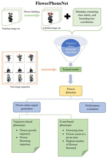
As with all deep-learning-based approaches, training is an essential process in FlowerPhenoNet. After the network is trained, a test image sequence of a plant is used to locate the flowers in each image and evaluate the performance of the network. Then, a set of novel temporal flower-based phenotypes are computed. Figure 2 shows the schematic of the FlowerPhenoNet system. Each of the steps is described next.

4.1. Image Labeling

We randomly selected 300 images from the dataset (100 images from each of the three flowering plant species, i.e., sunflower, canna, and coleus) containing multiple views of a set of plants for training the network. The plants were at different stages of growth bearing flowers from emergence to full bloom. Thus, the training set consists of a range of images containing buds to full-grown flowers, which is an essential criterion to achieve the goal of flower emergence timing detection and flower growth monitoring. Figure 3 shows some sample labeled images of the training set. The flowers in the training set are manually enclosed by rectangular boxes (shown in red) using the open source image annotation tool called ‘LabelImg’ [19].

4.2. Data Augmentation

Deep convolutional neural networks perform remarkably well on many computer vision tasks, e.g., image segmentation, image classification, and object detection. However, these networks are heavily reliant on large training datasets to combat overfitting by increasing the generalizability of the models [20]. Data augmentation strategy encompasses a suite of techniques to increase the size and quality of the training sets by usually applying various geometric and photometric transformations to the original labeled images during training [20]. It helps in adding more variety to the training set without actually having to increase the number of labeled training samples. In this method, the images in the training set are first cropped and then labeled for flowers before being subjected to augmentation. In FlowerPheno, data augmentation is performed after flower samples are labeled prior to training the network. The transformations used in this step include random horizontal flipping, scaling, and changing contrast. Figure 4 shows the results of data augmentation strategies used in FlowerPhenoNet. Note that test images are supposed to be representative of the original images without any alteration, and hence, must not be subjected to data augmentation for unbiased evaluation.

4.3. Neural Network Architecture and Training

Flower detection can be logically mapped to the object detection problem that has been widely studied in computer vision using both traditional and deep learning approaches. Object detection typically entails identifying the presence of the object, its location, and its type. YOLO (You Only Look Once) is a fast object detection algorithm proposed by [21] for real-time processing that has been widely used in a variety of applications. It is a one-stage object detection method that makes predictions of bounding boxes and class probabilities simultaneously by using an end-to-end neural network. Its architecture consists of a feature extraction network followed by a detection network. Thus, YOLO has a better inference speed than the two-stage models (e.g., R-CNN, Fast R-CNN, and Faster R-CNN). YOLOv3 used in this research uses the Darknet-53 [22] network which has 53 convolution layers with residual blocks. Residual blocks are used in deep neural networks to avoid saturation of accuracy with increasing depth.

The performance of the YOLO detector depends heavily on the quality of the labeling, i.e., masks generated from the images in the training dataset corresponding to different instances of the classes. Many open-source tools are available to generate the masks effectively. In this research, we have used the ‘LabelImg’ [19], a graphical image annotation tool, that generates the masks in the ‘YOLO’ format and hence can be fed directly into the YOLO architecture for training. Then, the images, along with their corresponding masks (ground-truth) are used to train the Darknet-53 framework, the core of the YOLOv3 architecture. The network is pre-trained on the COCO dataset [23] consisting of 80 classes. We then retrained the network with our labeled training data. Some important hyperparameters specified in our configuration include batch size (set to 32), max batches (set to 2000), and the number of filters (set to 18). The updated weights in the network were saved after 3000 epochs to constitute the FlowerPhenoNet.

YOLOv4 and YOLOv5 share the same head and neural network type as YOLOv3, but differ in the backbone, neck, and loss function ([24]). While YOLOv3 uses Darknet53 as the backbone, YOLOv4 uses CSPDarknet53. YOLOv5 uses a Focus structure with CSPdarknet53 as a backbone where the Focus layer evolved from YOLOv3. YOLOv5 replaces the first three layers of YOLOv3 to create a single focus layer. Most of the comparative studies among YOLOv3, YOLOv4, and YOLOv5 reported that YOLOv4 and YOLOv5 outperformed YOLOv3 in terms of accuracy but at the expense of slower inference speed [25]. Since the goal of FlowerPhenoNet is not to provide comparative performance analysis among different versions of YOLO for flower detection but to demonstrate the efficacy of the algorithm to compute temporal flower phenotypes for characterizing a plant’s vigor, we choose YOLOv3 for our application. YOLOX also uses YOLOv3 with Darknet-53 backbone and spatial pyramid pooling (SPP) layer as the baseline, but it is anchor-free [25]. Since anchors play a vital role in FlowerPhenoNet, YOLOX is not a feasible option.

Modern deep-learning-based object detectors make use of anchor boxes to predict the location and size of an object in an image accurately with faster speed [26]. A detailed description of the anchor box optimization technique used in FlowerPhenoNet to automatically learn the shapes of anchors during training can be found in [26]. Choosing the number of anchors is an important training hyperparameter that requires careful consideration and is determined using empirical analysis. Note that a value greater than 0.5 for mean IoU implies that the anchor boxes overlap well with the bounding boxes of the training samples. Figure 5 shows the mean intersection-over-union (IoU) versus the number of anchors. It is clear from the figure that the mean IoU can be improved if the number of anchor boxes is increased; however, using more anchor boxes in an object detector can also increase the computational complexity and lead to overfitting, which results in poor detection performance. In Figure 5, mean IoU shows an upward trend until the number of anchor boxes reaches 9, and then drops to a lower value at the number of anchor boxes 10 before it continues to remain somewhat steady. To make a trade-off between the computational complexity and the performance, we chose the value of the number of anchor boxes to be 9.

4.4. Testing and Evaluation

For testing the performance of the flower detector, we used an image sequence consisting of images of all days for available views of a plant. The test images are resized to match the size of the images in the training set. We have used IoU, confidence score (CS), and precision–recall curve as our evaluation metrics. IoU is an evaluation metric used to measure the accuracy of an object detector on a particular dataset. IoU is computed using Equation (1) where the numerator is the area of overlap between the predicted bounding box and the ground-truth bounding box. The denominator is the area of the union of the predicted bounding box and the ground-truth bounding box.

$$IoU=\frac{AreaofOverlap}{AreaofUnion}$$

(1)

The confidence score, CS, is the probability that an anchor box contains an object. It is usually predicted by a classifier. It is calculated using Equation (2) as follows:

$$CS=P\left(Object\right)\times IoU$$

(2)

where $P\left(Object\right)$ is the probability of a predicted bounding box containing an object.

We use the average precision metric to evaluate the performance of the algorithm. The average precision is a single number that incorporates the ability of the detector to make correct classifications, i.e., precision, and the ability of the detector to find all relevant objects, i.e., recall, which is computed as the area under the precision–recall curve. The precision/recall curve highlights how precise a detector is at varying levels of recall. The ideal value of precision is 1 at all levels of recall, i.e., the area under the curve equals 1.

4.5. Phenotype Computation

After the flowers are detected in the plant images, FlowerPhenoNet generates a flower status report consisting of the following temporal phenotypes.

4.5.1. Trajectory-Based

In an HTP3, a plant is imaged at regular intervals for a significant period of its life cycle to capture salient information about its development. The phenotypes computed by analyzing each image of the sequence can therefore be represented as a discrete time series, mathematically represented by, $p_1,p_2,\dots ,p_n$, where $p_i$ denotes the phenotype p for the i-th image of the plant (which is also the i-th timestamp), and n is the number of times the plant was imaged and hence is the length of the sequence [27]. A set of phenotypes computed from a time series of plant images is called a trajectory-based phenotype. Trajectory-based phenotypes are often represented graphically for visualization. In this research, we compute two trajectory based phenotypes, i.e., flower growth trajectory and blooming trajectory. Flower growth trajectory or flower blooming trajectory is formally denoted by the graphical representation of $p_1,p_2,\dots ,p_n$, where $p_i$ represents the flower size (for flower growth trajectory) or total flower count (for flower blooming trajectory) for the i-th image of the plant.

4.5.2. Event-Based

Event-based phenotype reports the timing (i.e, the day of imaging) of the significant events of a plant’s life cycle, i.e., the timing of transition from the vegetative stage to the reproductive stage by the emergence of the first flower. Thus, the flower status report consists of the following phenotypes, i.e., the timing of emergence of the first flower, the total number of flowers present at any given time in the image sequence, the size of each flower, flower growth trajectory, and the highest number of flowers bloomed in the plant during its life cycle.

5. Experimental Design and Analysis

The performance of FlowerPhenoNet is evaluated based on experimental analysis of the FlowerPheno dataset for (a) flower detection and (b) phenotype computation.

5.1. Flower Detection

Figure 6 and Figure 7 show the image sequences of a sunflower plant (Plant-ID D2) captured from a side view and the top view, respectively, along with the detected sunflowers. The figures show that multiple flowers with different sizes and orientations are efficiently detected.

Figure 8 shows the precision/recall curve for the sunflower test sequence shown in Figure 6. The average precision for all images of this sequence is 0.93. Canna and coleus plants are considered to be characterized by the presence of a single flower in an image. FlowerPhenoNet was able to detect all of them for all image sequences of FlowerPheno dataset. Hence, for canna and coleus, we show the IoUs against days for different view angles. Figure 9 and Figure 10 show the IoUs against different days for a canna and a coleus image sequence, respectively. The figures show that the IoU values lie in the range of [0.6, 0.95], where majority of them are above 0.75.

Figure 11 shows the average precision and mean IoU for all 20 sunflower plants from the FlowerPheno dataset. Mean IoU is computed by taking the mean of IoUs of all flowers in a given image. The figure shows that average precision lies in the range [0.89, 0.94], whereas mean IoU reports a slightly lower range of values, i.e., [0.816, 0.835].

Figure 12 and Figure 13 show the image sequences of a canna plant (Plant-ID D1) captured from the side view 0${}^{°}$ and the top view, respectively, along with the detected canna flower in each image. The confidence score is shown on the top of the bounding rectangle enclosing each detected flower. For the side view 0${}^{°}$, the confidence score lies in the range of [0.980, 0.999] (Figure 12), while in the case of the top view (Figure 13), the confidence score lies in the range of [0.621, 0.988].

Similarly, Figure 14 and Figure 15 show the image sequences of a coleus plant (Plant-ID D1) captured from the side view 0${}^{°}$ and the top view, respectively, along with the detected flowers in each image. The figures show a very high range of confidence scores for both the side view and the top view, in the range of [0.911, 0.999]. In summary, the results demonstrate the efficacy of FlowerPhenoNet in detecting flowers in three diverse species, where the flowers are detected even at very early stages of appearance.

5.2. Phenotype Computation

The flower emergence day of a plant is defined as the day on which the flower is first detected in the image sequence. It is clear from Figure 6 that the day of the first appearance of the flower as detected by the FlowerPhenoNet is Day 15; however, Figure 7 reports that Day 17 is the day on which the flower is first detected in this plant.

The 3D bar graphs in Figure 16a,b represent the flower status graphs for two sample sunflower plants (plant-IDs D5 and D6, respectively). The flower status graph provides important information including (a) the emergence day of the flower in each view; (b) the total number of flowers present in the plant for a given view on any day; and (c) the highest number of flowers bloomed in the plant. The 3D bars in the graph represent the number of flowers present in the plant image sequence in all views. It is clear from Figure 16b that Day 13 is the earliest when flowers are first detected in the image sequence (reported by side view 144${}^{°}$ and the top view). Hence, Day 13 is denoted as the flower emergence day for this plant. Note that all views report the existence of at least one flower for this plant on Day 16. The flower status graph reports the number of flowers present in all views and helps us determine the highest number of flowers in the plant on a given day. For example, the highest number of flowers on Day 19 is 4. The highest number of flowers blooming in the plant is 5, and that first appeared on Day 20 in several views. For plant-ID D5 (see Figure 16a), the top-view first shows a detected flower on Day 12, and hence, Day 12 is noted as the flower emergence day for this plant. Again, all views report the existence of at least one flower for this plant on Day 15. The highest number of flowers blooming in this plant is 7, and they first appeared on Day 20 in the top view.

The size of the flower is measured by the area of the bounding rectangle enclosing the detected flower in the image. The flower size as a function of time is represented as the flower growth trajectory. Note that drooping of petals, frequent change in orientation of flowers, and partial occlusions of flowers by leaves pose challenges in the accurate estimation of flower size based on area measurement from a 2D image. The computation of flower growth trajectory is not applicable for the flowers, which change their orientation frequently (e.g., sunflower). because, for those cases, the area of the bounding rectangle enclosing a detected flower in the time series image data changes in accordance to the change of orientation of the flower, and hence, is not a representation of the growth of the flower; thus, this paper uses coleus and canna to demonstrate the flower growth trajectory. Figure 17 and Figure 18 show the growth trajectories of coleus and canna flowers for five side views and the top view, respectively. The five side views are chosen alternatively from the sequence of side views in the FlowerPheno dataset such that they cover the range [0${}^{°}$, 360${}^{°}$] with uniform view interval. The results show an overall increasing trend in flower size for both canna and coleus flowers for most views.

The experimental analyses were performed using the Kaggle Notebook, a free cloud computing platform that allows executing code using dedicated GPUs. We used a GPU Kernel with Tesla P100 16 GB VRAM as GPU, with 13 GB RAM and a 2-core Intel Xeon as CPU. The training data were generated using the open-source image annotation tool called ‘LabelImg’. FlowerPhenoNet is implemented in Python programming language which is featured with a plethora of useful packages, e.g., OpenCV, TensorFlow, Keras, Scikit-learn, etc. The number of images used for training is 300. The execution time for training the FlowerPhenoNet is 1.5 h.

6. Discussion

Flowering plants (angiosperms) emerged on our planet approximately 140 to 160 million years ago and currently, they represent about 90% of the more than 350,000 known plant species [28]. Flowers are the reproductive organs of a plant and play a critical role in the production of fruits and seeds. The transition timing of vegetative meristems to the formation of flowers and their morphological development manifested in shape, size, and color provide crucial information about a plant’s vigor. Hence, the study of flower-based phenotyping is important in the understanding of plant growth processes. Furthermore, the timing of flowering is critical for reproductive success in many plant species. For example, flowering must occur early enough in the growing season to enable proper seed development, but premature flowering when a plant is small will limit the amount of seed that can be produced [29].

The proposed algorithm is applicable to a wide variety of flower species with varying shapes, architectures, and growth patterns, using images captured in an HTP3. In this paper, we focus on three representative flowering plant species, i.e., sunflower, canna, and coleus, which pose different computer vision challenges due to their variations in architectures, and thus, enable us to establish the robustness of the proposed method. Sunflower is an economically important crop primarily used as a source of edible oil, and sunflower seeds are used for food as well. One of the fastest-growing plants, sunflowers, is often used by farmers to feed livestock. A sunflower plant is characterized by the presence of multiple flowers that rotate to align with the direction of incident sunlight. Canna is a tropical plant with gladiolus-like flower spikes that bloom atop erected stems. It is one of the most popular garden plants; however, in some parts of the world, its rhizomes are consumed as a source of starch. Canna seeds are also used as beads in jewelry. Coleus is a plant that has been used since ancient times to treat heart disorders such as high blood pressure and chest pain (angina) and respiratory disorders such as asthma. In the FlowerPheno dataset, both canna and coleus plant images are considered to have single composite flowers.

With the enormous growth of the processing capability of computers, deep learning has been impacting the world in recent times, replacing traditional approaches to solving computer vision tasks. For the task of object detection, as in FlowerPhenoNet, the traditional image analysis pipelines consist of low-level image processing steps followed by intermediate-level feature extraction and ending with a classifier. State-of-the-art computer vision systems overwhelmingly use end-to-end learning that directly maps images to class labels using deep neural networks. Deep neural networks are characterized by a structure that contains a lot of layers, and in each layer, neurons are able to implicitly represent features from the data that propagate to the next layer [30]. In this way, more complex information can be obtained in later layers, and image features are automatically determined by the network. These systems have demonstrated superiority over traditional approaches for a wide variety of tasks, in many cases matching the performance of humans.

This paper introduces a novel deep-learning-based framework called FlowerPhenoNet to detect flowers in an image sequence and generate a flower status report consisting of a set of novel temporal flower phenotypes. The paper also introduces a benchmark dataset to allow further development of new methods and provide a common basis for uniform comparison of the state-of-the-art methods. The dataset consists of three representative flowering plant species, i.e., sunflower, canna, and coleus. These three different species of plants have different architectures and flowering patterns. The shapes and textures of their flowers are also different. The demonstrated high performance of FlowerPhenoNet on this dataset shows its potential applicability to a wide variety of flower species with different shapes and topologies.

Plants are not static but living organisms that change in shape and topology over time. The occlusions of flowers by the leaves, drooping of petals, and change in orientation of flowers in accordance with the incident sunlight pose challenges to the accurate computation of flower size from 2D images. In general, it is not feasible to compute the growth trajectory of a sunflower from any single view image (based on estimating the area of its enclosed bounding rectangle), as the sunflower changes its orientation based on incident sunlight at different times of the day, resulting in the change in the area of the bounding rectangle in accordance with flower rotation but not its growth. Thus, to accurately estimate the size, our future work will consider the 3D model reconstruction of the sunflowers using multiview images. In addition to the change in orientation, the occlusion of flowers by leaves also poses challenges to flower size estimation, and, consequently, computation of flower growth trajectory. Since different parts of a plant generate unique reflectance patterns in different image spaces, we will explore hyperspectral imagery in future work to address this occlusion issue. Note that our proposed method shows a consistent overall increasing trend of flower growth for coleus and canna because these two plants are not considerably affected by changes in orientation and occlusion of flowers by leaves (see Figure 17 and Figure 18).

The highest number of flowers blooming in the plant is estimated by the maximum number of flowers visible in any view in any image of the sequence. Although this assumption holds true for all sunflower plants in the FlowerPheno dataset; however, there might be cases where the image view with the maximum number of flowers excludes a few flowers that are visible in other views; thus, future work will consider view registration to ensure all flowers are counted accurately to report the highest number of flowers blooming in the plant.

7. Conclusions

The transition timing of vegetative meristems to the formation of flowers and their morphological development over time plays a significant role in yield estimation and breeding. The paper introduces a novel deep-learning-based system called FlowerPhenoNet for monitoring flower-based phenotypes using time-series images captured in an HTP3. FlowerPhenoNet uses the YOLOv3 [21] deep-learning-based object detector to locate flowers in the multiview image sequence for application in temporal plant phenotyping. A benchmark dataset is indispensable for new algorithm development, performance evaluation, and uniform comparisons among the existing algorithms. To support this goal, we publicly introduce a benchmark dataset called FlowerPheno comprising visible light image sequences of sunflower, canna, and coleus plants captured from multiple viewing angles in the LemnaTec Scanalyzer 3D HTP3. Following flower detection, FlowerPhenoNet generates a flower status report consisting of a set of novel temporal phenotypes, e.g., the day of emergence of the first flower in a plant’s life cycle, the total number of flowers present in the plant at a given time, the highest number of flowers bloomed in the plant, flower growth trajectory, and blooming trajectory. In this paper, the efficacy of FlowerPhenoNet is demonstrated using experimental analysis on three flowering plant species, namely sunflower, canna, and coleus; however, the method has the potential to be applied to a wide variety of species with varying shapes, architectures, and growth patterns. In future work, we will consider augmenting the FlowerPheno dataset to include images of more flowering plant species captured from multiple side views in the HTP3 of UNL. We will perform a comparative analysis in terms of flower detection accuracy and speed using newer object detection networks that have evolved from YOLOv3, i.e., YOLOv4, YOLOv5, YOLOX, etc., using the augmented dataset. Future work will also consider the 3D model reconstruction of the flowering plants to achieve accuracy in flower size estimation, and counting of the highest number of flowers bloomed in the plant.

References

- Das Choudhury, S.; Bashyam, S.; Qiu, Y.; Samal, A.; Awada, T. Holistic and Component Plant Phenotyping using Temporal Image Sequence. Plant Methods 2018, 14, 35. [Google Scholar] [CrossRef] [PubMed]
- Das Choudhury, S.; Samal, A.; Awada, T. Leveraging Image Analysis for High-Throughput Plant Phenotyping. Front. Plant Sci. 2019, 10, 508. [Google Scholar] [CrossRef] [PubMed]
- Samal, A.; Das Choudhury, S.; Awada, T. Image-Based Plant Phenotyping: Opportunities and Challenges. In Intelligent Image Analysis for Plant Phenotyping; Samal, A., Das Choudhury, S., Eds.; CRC Press, Taylor & Francis Group: Boca Raton, FL, USA, 2020; pp. 3–23. [Google Scholar]
- Xu, R.; Li, C.; Paterson, A.H.; Jiang, Y.; Sun, S.; Robertson, J.S. Aerial Images and Convolutional Neural Network for Cotton Bloom Detection. Front. Plant Sci. 2018, 8, 2235. [Google Scholar] [CrossRef] [PubMed] [Green Version]
- Santad, T.; Silapasuphakornwong, P.; Sookhanaphibarn, K.; Choensawat, W. Application of YOLO Deep Learning Model for Real Time Abandoned Baggage Detection. In Proceedings of the IEEE 7th Global Conference on Consumer Electronics (GCCE), Nara, Japan, 9–12 October 2018; pp. 157–158. [Google Scholar]
- Song, H.; Liang, H.; Li, H.; Dai, Z.; Yun, X. Vision-based vehicle detection and counting system using deep learning in highway scenes. Eur. Transp. Res. Rev. 2019, 11, 51. [Google Scholar] [CrossRef] [Green Version]
- Wang, Z.; Walsh, K.; Koirala, A. Mango Fruit Load Estimation Using a Video Based MangoYOLO—Kalman Filter—Hungarian Algorithm Method. Sensors 2019, 19, 2742. [Google Scholar] [CrossRef] [PubMed] [Green Version]
- Kuhn, H.W. The Hungarian Method for the assignment problem. Nav. Res. Logist. Q. 1955, 2, 83–97. [Google Scholar] [CrossRef] [Green Version]
- Kalman, R.E. A New Approach to Linear Filtering and Prediction Problems. Trans. ASME–J. Basic Eng. 1960, 82, 35–45. [Google Scholar] [CrossRef] [Green Version]
- Afonso, M.; Fonteijn, H.; Fiorentin, F.S.; Lensink, D.; Mooij, M.; Faber, N.; Polder, G.; Wehrens, R. Tomato Fruit Detection and Counting in Greenhouses Using Deep Learning. Front. Plant Sci. 2020, 11, 1759. [Google Scholar] [CrossRef] [PubMed]
- Mai, X.; Zhang, H.; Jia, X.; Meng, M.Q.H. Faster R-CNN With Classifier Fusion for Automatic Detection of Small Fruits. IEEE Trans. Autom. Sci. Eng. 2020, 17, 1555–1569. [Google Scholar] [CrossRef]
- Bargoti, S.; Underwood, J. Deep fruit detection in orchards. In Proceedings of the IEEE International Conference on Robotics and Automation, Singapore, 29 May–3 June 2017; pp. 3626–3633. [Google Scholar] [CrossRef]
- Li, Y.; Fan, X.; Mitra, N.J.; Chamovitz, D.; Cohen-Or, D.; Chen, B. Analyzing Growing Plants from 4D Point Cloud Data. ACM Trans. Graph. 2013, 32, 1–10. [Google Scholar] [CrossRef]
- Agarwal, B. Detection of Plant Emergence Based on Spatio Temporal Image Sequence Analysis. Master’s Thesis, The University of Nebraska-Lincoln, Lincoln, NE, USA, 2017. [Google Scholar]
- Scharr, H.; Bruns, B.; Fischbach, A.; Roussel, J.; Scholtes, L.; Stein, J.V. Germination Detection of Seedlings in Soil: A System, Dataset and Challenge. In Proceedings of the Computer Vision—ECCV 2020 Workshops; Bartoli, A., Fusiello, A., Eds.; Springer International Publishing: Berlin/Heidelberg, Germany, 2020; pp. 360–374. [Google Scholar]
- Bashyam, S.; Das Choudhury, S.; Samal, A.; Awada, T. Visual Growth Tracking for Automated Leaf Stage Monitoring Based on Image Sequence Analysis. Remote Sens. 2021, 13, 961. [Google Scholar] [CrossRef]
- Das Choudhury, S.; Goswami, S.; Bashyam, S.; Samal, A.; Awada, T. Automated Stem Angle Determination for Temporal Plant Phenotyping Analysis. In Proceedings of the IEEE International Conference on Computer Vision workshop on Computer Vision Problmes in Plant Phenotyping, Glasgow, UK, 28 August 2020; pp. 41–50. [Google Scholar]
- Lu, H.; Cao, Z.; Xiao, Y.; Zhuang, B.; Shen, C. TasselNet: Counting maize tassels in the wild via local counts regression network. Plant Methods 2017, 13, 79. [Google Scholar] [CrossRef] [PubMed] [Green Version]
- Tzutalin. LabelImg. Free Software: MIT License. 2015. Available online: https://www.bibsonomy.org/bibtex/24d72bded15249d2d0e3d9dc187d50e16/slicside (accessed on 3 January 2019).
- Shorten, C.; Khoshgoftaar, T.M. A survey on Image Data Augmentation for Deep Learning. J. Big Data 2019, 6, 1–48. [Google Scholar] [CrossRef]
- Redmon, J.; Farhadi, A. YOLO9000: Better, Faster, Stronger. In Proceedings of the 2017 IEEE Conference on Computer Vision and Pattern Recognition (CVPR), Honolulu, HI, USA, 21–26 July 2017; pp. 6517–6525. [Google Scholar]
- Mao, Q.C.; Sun, H.M.; Liu, Y.B.; Jia, R.S. Mini-YOLOv3: Real-time object detector for embedded applications. IEEE Access 2019, 7, 133529–133538. [Google Scholar] [CrossRef]
- Lin, T.Y.; Maire, M.; Belongie, S.; Hays, J.; Perona, P.; Ramanan, D.; Dollár, P.; Zitnick, C.L. Microsoft coco: Common objects in context. In Proceedings of the European Conference on Computer Vision; Springer: Berlin/Heidelberg, Germany, 2014; pp. 740–755. [Google Scholar]
- Nepal, U.; Eslamiat, H. Comparing YOLOv3, YOLOv4 and YOLOv5 for Autonomous Landing Spot Detection in Faulty UAVs. Sensors 2022, 22, 464. [Google Scholar] [CrossRef] [PubMed]
- Ge, Z.; Liu, S.; Wang, F.; Li, Z.; Sun, J. YOLOX: Exceeding YOLO Series in 2021. arXiv 2021, arXiv:2107.08430. [Google Scholar]
- Zhong, Y.; Wang, J.; Peng, J.; Zhang, L. Anchor Box Optimization for Object Detection. In Proceedings of the IEEE/CVF Winter Conference on Applications of Computer Vision (WACV), Snowmass Village, CO, USA, 1–5 March 2020. [Google Scholar]
- Das Choudhury, S. Time Series Modeling for Phenotypic Prediction and Phenotype-Genotype Mapping Using Neural Networks. In Proceedings of the Computer Vision—ECCV 2020 Workshops; Bartoli, A., Fusiello, A., Eds.; Springer International Publishing: Cham, Switzerland, 2020; pp. 228–243. [Google Scholar]
- Paton, A.J.; Brummitt, N.; Govaerts, R.; Harman, K.; Hinchcliffe, S.; Allkin, B.; Lughadha, E.N. Towards Target 1 of the Global Strategy for Plant Conservation: A working list of all known plant species—progress and prospects. TAXON 2008, 57, 602–611. [Google Scholar] [CrossRef]
- Amasino, R.M.; Cheung, A.Y.; Dresselhaus, T.; Kuhlemeier, C. Focus on Flowering and Reproduction. Plant Physiol. 2017, 173, 1–4. [Google Scholar] [CrossRef] [PubMed] [Green Version]
- Ubbens, J.R.; Stavness, I. Deep Plant Phenomics: A Deep Learning Platform for Complex Plant Phenotyping Tasks. Front. Plant Sci. 2017, 8, 1190. [Google Scholar] [CrossRef] [PubMed]
Figure 1.
LemnaTec Scanalyzer 3D high-throughput plant phenotyping facility at the UNL: view of the automated greenhouse (top-left); watering station (top-right); a plant entering the fluorescent chamber (bottom-left); and plants on the conveyor belt heading towards the visible light chamber (bottom-right).
Figure 2.
Block diagram of FlowerPhenoNet.
Figure 3.
Sample labeled multi-view images from FlowerPheno dataset used for training: Coleus (row-1); Canna (row-2); and Sunflower (row-3). Top-view (column-1); Side-view (column-2); Side-view (column-3); Side-view (column-4).
Figure 4.
Illustration of data augmentation strategies using transformations and illumination alteration: original image (top-left); scaled image (top-right); reflected image (bottom-left) and illumination altered image (bottom-right).
Figure 5.
Mean IoU versus number of anchors: determination of the number of anchor boxes using a sunflower test sequence by analyzing the evaluation metric mean IoU.
Figure 6.
Illustration of flower emergence timing detection using a sample sunflower image sequence (D2) for the side view 0 over consecutive days (following left to right direction) starting from Day 10 (top-left) to Day 24 (bottom-right).
Figure 7.
Illustration of flower emergence timing detection using a sample sunflower image sequence (D2) for the top view over consecutive days (following left to right direction) starting from Day 16 (top-left) to Day 27 (bottom-right).
Figure 8.
The precision/recall curve for a sunflower test sequence.
Figure 9.
Performance analysis using IoU for a canna image sequence for multiple views (Plant-ID: Canna-C1).
Figure 10.
Performance analysis using IoU for a coleus image sequence for multiple views (Plant-ID: Coleus-D1).
Figure 11.
Flower detection performance of sunflower plants from FlowerPheno dataset using average precision and mean IoU.
Figure 12.
Illustration of flower emergence timing detection and its growth over consecutive days (following left to right direction) using a sample canna image sequence (D1) for the side view 0 starting from Day 28 (top-left) to Day 35 (bottom-right).
Figure 13.
Illustration of flower emergence timing detection and its growth over consecutive days (following left to right direction) using a sample canna image sequence (D2) for the top view starting from Day 28 (top-left) to Day 35 (bottom-right).
Figure 14.
Illustration of flower emergence timing detection and its growth over consecutive days (following left to right direction) using a sample Coleus image sequence (D2) for the side view 0 starting from Day 16 (top-left) to Day 33 (bottom-right).
Figure 15.
Illustration of flower emergence timing detection and its growth over consecutive days (following left to right direction) using a sample Coleus image sequence (D2) for the top view starting from Day 16 (top-left) to Day 33 (bottom-right).
Figure 16.
The flower status graphs for two sample sunflower plants: (a) Plant-ID D5; (b) Plant-ID D6.
Figure 17.
Illustration of the growth trajectory of a canna flower in multiple views (Plant-ID: Canna-D1).
Figure 18.
Illustration of the growth trajectory of a coleus flower in multiple views (Plant-ID: Coleus-D1).