


Application of Soil Moisture Active Passive (SMAP) Satellite Data in Seismic Response Assessment

Department of Civil and Environmental Engineering, University of New Hampshire, Durham, NH 03824, USA
*
Author to whom correspondence should be addressed.
Remote Sens. 2022, 14(17), 4375; https://doi.org/10.3390/rs14174375
Submission received: 29 July 2022
/
Revised: 26 August 2022
/
Accepted: 30 August 2022
/
Published: 2 September 2022
(This article belongs to the Special Issue Satellite Soil Moisture Validation and Applications)
Abstract
:The proven relationship between soil moisture and seismic ground response highlights the need for a tool to track the Earth’s surface soil moisture before and after seismic events. This paper introduces the application of Soil Moisture Active Passive (SMAP) satellite data for global soil moisture measurement during earthquakes and consequent events. An approach is presented to study areas that experienced high level of increase in soil moisture during eleven earthquakes. Two ancillary datasets, Global Precipitation Measurement (GPM) and Global Land Data Assimilation (GLDAS), were used to isolate areas that had an earthquake-induced increase in soil moisture from those that were due to hydrological processes. SMAP-based soil moisture changes were synthesized with seismic records developed by the United States Geological Survey (USGS), mapped ground failures in reconnaissance reports, and surface changes marked by Synthetic Aperture Radar (SAR)-based damage proxy maps. In the majority of the target earthquakes, including Croatia 2020, Greece 2020, Indonesia 2018, Taiwan 2016, Ecuador 2016, and Nepal 2015, a relationship between the SMAP soil moisture estimates and seismic events was evident. For these events, the earthquake-induced soil moisture response occurred in liquefaction-prone seismic zones. The New Zealand 2016 event was the only study region for which there was a clear inconsistency between and the seismic records. The promising relationship between soil moisture changes and ground deformations indicates that SMAP would be a useful data resource for geotechnical earthquake engineering applications and reconnaissance efforts.
1. Introduction
Soil moisture impacts site characteristics including soil strength, stiffness, and damping due to the presence of inter-particle suction stresses [1,2,3,4]. Changes in the dynamic soil properties influence the seismic response of geotechnical systems such as site response, soil–structure interaction, and ground failure [5,6,7,8,9,10,11]. In addition, seismic events can cause an increase in soil moisture content, resulting in ground deformations and subsequent damage to infrastructure in extreme conditions [12,13,14,15]. This relationship between soil moisture and seismic response underscores the importance of studying the pre- and post-event soil moisture content in earthquake-hit regions. For example, the impact of the initial soil degree of water saturation on seismic compression and the consequent changes in water content have received significant attention in recent years [16,17,18,19,20]. These include the impacts of induced strain levels, soil volumetric deformation characteristics, fines content, and state of saturation. Partially saturated sands subjected to seismic compression experience an increase in degree of saturation [20].
Remotely sensed and in situ soil-moisture-measurement approaches have been widely used over the past decades [21,22,23]. Due to challenges in sensor installation, data collection, and maintenance [21], there are a limited number of large-scale in situ soil-moisture-monitoring networks, and these measurements are unlikely to be available to provide the required and immediate estimation of soil moisture before and after a seismic event. Within this context, well-calibrated remote sensing methods can provide effective alternative solutions to understand and evaluate the interaction between soil moisture and earthquake response at global scales.
Remote sensing has been used in recent decades to study geohazards such as earthquakes, volcanic eruptions, floods, and landslides [24,25,26,27,28,29]. Natural hazards assessments have benefited from remote sensing data for post-event surface damage detection [30,31,32,33], geodetic observations of volcanoes using GPS and InSAR [34], passive microwave measurements of precipitation that are applicable to improve flood forecasting [35,36], and remotely sensed soil moisture products used for analyzing landslide events [24,37,38,39].
For earthquake engineering, remote sensing techniques have been utilized to appraise different aspects of an event such as liquefaction, landslides, ground displacement, and infrastructure damage assessment [40,41,42,43]. Optical imagery has been widely used to identify ground failures [31,42] as well as structural damage [44,45]. However, optical imagery is limited by atmospheric conditions and may not have the temporal resolution and availability for pre- and post-earthquake data. Synthetic aperture radar (SAR) has also provided a tool to measure ground movements [46], detect surface changes [40], and identify structural damage [47] by measuring the reflections from its transmitted signals as well as advanced data-processing techniques [42]. Table 1 presents a summary of the satellite data used to develop remote sensing methods for the assessment of earthquake events, and their applications and challenges.
Due to the limited availability of in situ soil saturation measurements at large spatial scales, which are essential for a liquefaction or landslide probability assessment, parameters such as water table depth, precipitation measurements, and topographic conditions have been used as proxies for soil saturation to model and investigate geotechnical engineering events such as landslide and liquefaction [12,56]. Satellite image processing using thermal, near-infrared and shortwave infrared indicators as proxies for soil wetness have successfully mapped highly liquefied regions after earthquakes [25,31]. However, to date, direct observations of space-borne soil moisture data have not been used for seismic response analysis and geotechnical applications, which can be an alternative to the current proxies for soil saturation.
The Soil Moisture Active Passive [57] Earth observing satellite mission was launched in 2015 by National Aeronautics and Space Administration. SMAP detects soil moisture content in approximately the top 5 cm of the soil layer [58]. With near-global coverage, SMAP’s L-band radiometer measures the brightness temperature of Earth’s surface and estimates land surface conditions, such as vegetation water content and soil roughness, and then it derives the land surface soil moisture [59]. SMAP revisits each region around the globe every 2–3 days (or sooner) to capture surface soil moisture conditions. Using the Backus–Gilbert optimal interpolation, SMAP retrieves the soil moisture at a resolution of 9 km, and has a finer spatial resolution as well as a higher accuracy than its predecessors, such as the Tropical Rainfall Measuring Mission (TRMM) and Advanced Microwave Scanning Radiometer 2 (AMSR-2) [60]. SMAP microwave observations have been widely validated since the relevant datasets were released in April 2015 [61,62]. SMAP offers rich scientific datasets that have been used in a range of applications; for example, weather and climate predictions [63], agricultural and food productivity [64], and natural hazard monitoring, such as floods and landslides [65,66]. However, this product has not been employed by the earthquake engineering community to advance the state of the knowledge and practice. Considering the role of soil moisture content in seismic ground response, the SMAP observations may help the community understand the interaction between soil moisture and earthquakes and evaluate how pre- and post-event soil moisture affects different aspects of earthquake-induced soil response.
While earthquake-induced soil moisture responses are well-understood, the soil moisture also changes due to precipitation, infiltration, and evapotranspiration. Thus, observed soil moisture changes must account for these responses in order to determine the net response due to an earthquake. Ancillary datasets are needed at the global scale to isolate earthquake-induced soil moisture changes. The Global Precipitation Measurement (GPM) datasets [67] and Global Land Data Assimilation (GLDAS) product [68] are two products available for this purpose. The GPM monitored precipitation, which is a pivotal factor in soil moisture content, throughout the study period (time interval between pre- and post-event SMAP data). The GLDAS model data are generated from a climatologically consistent atmospheric forcing dataset and soil moisture variations are simulated based on satellite and ground-based observational meteorological data products.
The main objective of this paper is to evaluate the potential application of SMAP to quantify surface soil moisture before and after earthquakes. The paper is organized as follows: First, the target earthquakes and the data used in this study are identified. Then, the soil moisture and rainfall data products and methods are described. The findings from the integration of soil moisture variations with seismic data are presented. Finally, the conclusions and some recommendations for future investigations are given.
2. Materials and Methods
2.1. Study Regions
To evaluate seismic-induced soil moisture variations, a set of recent earthquakes coinciding with SMAP’s lifespan from April 2015 to the present that are rich in recorded seismic data were identified. This study focused on seismic areas that experienced moderate to high-intensity earthquakes during the SMAP observation period. Three main criteria were considered for event selection: (1) target earthquakes had a moment magnitude greater than 6.0; (2) events are well-documented with post-event field investigations, seismic records, and site characterizations maps; and (3) high-quality SMAP data are available; for example, SMAP cannot measure soil moisture values when a region is covered by snow and SMAP data are not reliable if radio-frequency interference (RFI) corrupts the data in regions such as Japan [69]. The geographic location, the mainshock date, and the magnitude of the eleven target earthquakes are depicted in Figure 1. The wide temporal and spatial distribution of target earthquakes ensures that the observations from this study can be extended to other seismic events.
For each earthquake, a focus zone was determined that contains all regions having a Modified Mercalli Intensity (MMI) of 5 or greater, based on data reported by the United States Geological Survey [70]; an example for the Petrinja, Croatia 2020 earthquake is shown in Figure 2 (focus zones for other study regions are shown in Figure A1 of the electronic supplement).
2.2. Data and Processing
2.2.1. Seismic Records
Seismic activity data, reconnaissance reports, and remotely sensed damage assessments from multiple resources were collected for the target events in order to qualitatively assess the possible relations between the soil moisture content dynamics of the shallow surface and the geotechnical characteristics of the earthquakes. The USGS Earthquake Hazard Program Data Center provides comprehensive near-real-time seismic data. For this study, peak ground acceleration (PGA) and MMI contours and earthquake-induced ground failure (landslide and liquefaction) estimates, which are publicly available at the USGS [70], were collected and classified for each study region and focus zone.
For all the target earthquakes in this paper except the Petrinja, Croatia 2020 earthquake, Geotechnical Extreme Events Reconnaissance (GEER) Association, funded by the National Science Foundation (NSF), assembled reconnaissance teams to record geotechnical aspects of the events [71]. For the Petrinja, Croatia 2020 earthquake, the Structural Extreme Events Reconnaissance (StEER) product [72] was used in this study. These reconnaissance reports mainly reviewed the earthquake history and geologic background of the study regions and also mapped geotechnical and, in some cases, structural damage by on-ground mapping and/or aerial imagery using small unmanned aerial vehicles.
Following major natural events, NASA’s Advanced Rapid Imaging and Analysis [73] team produces damage proxy maps (DPM) to identify the extent of potentially damaged areas. These maps are produced based on synthetic aperture radar (SAR) images [40]. DPMs were downloaded and used for three seismic zones in this research, including Samos in Greece, Palu in Indonesia, and Accumoli in Italy [73].
2.2.2. Soil Moisture and Precipitation Data
SMAP soil moisture observations are the primary dataset used to identify earthquake-induced near surface moisture changes. Because this research aims to capture and study seismic-induced soil moisture changes, the effects of climatic variables such as precipitation and evaporation on the soil moisture variation should be separated. For this purpose, three datasets were adopted. Table 2 summarizes the spatial and temporal resolution of the data products used in this study. It should be noted that in the rest of this manuscript, the spatial resolution of the GLDAS and GPM are reported in km (i.e., approximately 25 km and 10 km, respectively). For the sake of consistency, converted from kg/m2 to cm3/cm3, soil moisture values reported by GLDAS are presented herein in volumetric form.
SMAP is an Earth observation satellite, launched in January 2015, that carries an L-band radiometer and radar designed to enhance the scientific understanding of the interrelation between the land surface soil moisture, the freeze–thaw state, and the atmosphere for monitoring natural hazards, improving climate forecasts, assisting agricultural productivity, and tracking the water cycle [61]. The radar could have provided SMAP observations with a much higher spatial resolution, but it stopped transmitting data in July 2015. Nevertheless, the radiometer still continues to operate and provide high-accuracy data. This radiometer has the potential to record the soil moisture data over the global land area, excluding regions masked by urban areas, snow and ice, or inland open water bodies, and mountainous or highly vegetated areas, and its measurements are independent of weather conditions and solar illumination [58]. This study used enhanced level-3 passive surface soil moisture data (L3_SM_P_E), which were retrieved by the SMAP radiometer that provides the soil moisture in the top 5 cm of the soil column [57]. The L3_SM_P_E includes soil moisture records at 6:00 AM or 6:00 PM local solar time (LST). This data product has a grid resolution of 9 km on Equal Area Scalable Earth 2.0 grids and a 3-day average temporal resolution. In this paper, version 5 of this data product was used, which is freely available from the National Snow and Ice Data Center (NSIDC) [74] in hierarchical data format version 5 (HDF5).
GLDAS, developed by NASA, is a robust tool to model global land surface states. GLDAS-2.1 is a generation of this system that combines satellite and ground-based observational meteorological data products, including precipitation, air temperature, surface pressure, solar radiation, and wind through land surface models to estimate near-real-time global land surface variables, such as soil moisture, soil temperature, evaporation, snowmelt, and canopy transpiration, among others. In other words, GLDAS-2.1 utilizes meteorological data as the inputs to land surface models to simulate land surface variables. Hence, it does not record the perishable seismic-induced soil moisture change, and it is an appropriate tool to separate earthquake-induced moisture changes from atmospherically induced changes. GLDAS-2.1 provides soil moisture products in four different soil layers, i.e., 0–10 cm, 10–40 cm, 40–100 cm, and 100–200 cm, with a spatial resolution of 25 km at 3-h time steps. For this study, soil moisture data in the top layer (0–10 cm) were downloaded in network common data form version 4 format (NetCDF4) [75].
GPM is a joint mission between international space agencies to observe the Earth’s precipitation. The Integrated Multi-Satellite Retrievals for GPM (IMERG) algorithm consolidates and calibrates datasets from the GPM satellite constellation to estimate precipitation over the Earth’s surface at a 10 km spatial resolution with a half-hour temporal resolution. The GPM (IMERG) Level 3 Version 06 Final Run precipitation product used in this study includes bias correction based on a monthly gauge analysis. Because there might be a lag between pre- and post-event SMAP-based soil moisture data, accumulated precipitation data in this time window for study regions, measured by GPM, were downloaded and processed. The GPM data are released in network common data form version 4 format (NetCDF4) [76].
Previous studies have shown that GLDAS and SMAP soil moisture products have similar spatial patterns and show good agreement with in situ soil moisture measurements, with both soil moisture datasets having an accuracy that is generally lower than 0.04 . [77,78,79]. As discussed earlier, GLDAS soil moisture simulations cannot reflect seismically induced soil moisture changes. Therefore, in this paper, to differentiate earthquake-induced soil moisture changes from climate-induced ones, the recorded moisture change data extracted from SMAP and GLDAS were compared.
2.2.3. SMAP Event Window
Considering the SMAP repeat frequency, there is a time interval of about 24 to 72 h between pre- and post-earthquake SMAP data. Table 3 lists the mainshock date and the pre- and post-event SMAP data available for each earthquake. To avoid the effects of diurnal cycles on soil moisture, only 6:00 AM SMAP surface soil moisture retrievals were used in this study and therefore, for each earthquake, the nearest available 6:00 AM SMAP data were selected for the analysis. For example, the Petrinja, Croatia 2020 earthquake happened at 11:20 AM coordinated local time [80], which equals 12:20 LST, on 29 December 2020. The nearest available SMAP data for the Croatia region before and after this earthquake were acquired on 29 December 2020 (6:00 AM LST) and 30 December 2020 (6:00 AM LST), respectively.
Because GLDAS has a three-hour temporal resolution, soil moisture data from this platform are available less than three hours before and after earthquakes. However, since pre- and post-event SMAP soil moisture data were being compared with the GLDAS data, the soil moisture products provided by GLDAS were downloaded for the same pre- and post-event dates and times as in SMAP. The SMAP data time interval (SMAP event window), dictated by the temporal resolution of SMAP, also determined the time period for which the accumulated precipitation data (GPM) were obtained for this study.
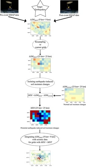
Soil moisture change () in the SMAP event window was calculated for both SMAP and GLDAS soil moisture products as follows:
where and are the soil moisture before and after the event, respectively. Figure 3 shows an example of maps calculated based on SMAP () and GLDAS () in their native spatial resolution, as well as the GPM accumulated precipitation in this time window for the Petrinja, Croatia 2020 earthquake.
2.2.4. Resampling to Coarser Grids
As shown in Table 2, the GLDAS data have the coarsest grid. For the sake of consistency of spatial resolution, SMAP and GPM data products were resampled to a spatial resolution matching GLDAS. For this purpose, the average resampling method was performed [81]. Figure 4 demonstrates examples of SMAP and GPM data products before and after the resampling.
3. Results
3.1. Relationship between ΔSM and GPM Data
Precipitation is the most important hydrological variable that influences the soil wetness condition, particularly for the near-surface. Both the GLDAS and SMAP soil moisture products effectively respond to atmospheric conditions [61,79]. Hence, a strong relationship should exist between values and the intensity and spatial pattern of rainfall events. While will follow this relationship, earthquake impacts on soil moisture may change this template for the observed . Figure 5 shows values from SMAP () and GLDAS (), as well as the amount of accumulated precipitation in the SMAP event window for some of the target earthquakes at a 25 × 25 km resolution, i.e., after resampling SMAP and GPM data to coarser grids (similar maps for other seismic zones are shown in Figure A2 of the supplement). In three of the study zones, including Meinong in Taiwan, Accumoli in Italy, and Samos in Greece, no significant rainfall was reported in the SMAP event window. While followed GPM, in which soil moisture decreased in these regions, the SMAP data showed considerable increases in soil moisture content for some grids. These increases were readily observed for many grids in Palu, Indonesia and Illapel, Chile as well. These results, in turn, suggest that SMAP can register earthquake-induced soil moisture increases.
3.2. Moisture Differences
The difference between the two sets of soil moisture change data, i.e., and , was used to identify the grids experiencing earthquake-induced soil moisture increases during seismic events. The moisture difference indicator () for each grid was expressed as follows:
Figure 6 shows the maps for all the study zones in the corresponding SMAP event window. In the Petrinja, Croatia 2020 earthquake, the is positive for most grids, meaning that the soil moisture change from SMAP () is higher than that from GLDAS ().
Because of the fundamental disparities between the methods used in SMAP and GLDAS, a difference between and might have existed even in the absence of the earthquake. For instance, for the vegetated areas with vegetation water contents more than 5 , such as forests and wetlands, SMAP can overestimate the soil moisture content [78]. Moreover, SMAP and GLDAS estimate the soil moisture for two different soil depths. Although previous studies showed strong correlations between the soil moisture of the soil columns, whether selected shallow or deep [82], this difference between shallow and deep soil moisture is still an uncertainty. GLDAS provides soil moisture values for a deeper soil layer, and it may show lower variability () in response to the atmospheric conditions [83]. Nevertheless, GLDAS helps to understand whether the SMAP increased soil moisture during the event window might be due to precipitation. To isolate the grids with a significant earthquake-induced soil moisture increase, a moisture difference threshold (MDT) was defined. In the grids for which the exceeds the MDT, the earthquake had a notable impact resulting in soil moisture increase.
Before choosing GLDAS for this study, GLDAS and SMAP were compared for longer periods in normal conditions (i.e., without an earthquake). For example, while grids with an MDI > 0.08 cm3/cm3 can be seen in the SMAP event window, the absolute values of the MDI in the absence of an earthquake in the central Croatia region under normal conditions are generally lower than 0.04 cm3/cm3. Moreover, the average absolute values of the MDI for grids of this region for the time period from January 2019 to December 2020 was approximately 0.028 cm3/cm3. However, because no verified or average value of MDT in the absence of earthquake has been reported in the literature, in this paper, several thresholds were evaluated. Threshold values, i.e., 0, 0.02, 0.04, and 0.08 , were used to identify the grids with a notable earthquake-induced soil moisture increase. Grids having an less than zero were neglected. This is a conservative assumption because in many cases the climate-induced soil moisture changes recorded by SMAP are less than that by GLDAS [78], i.e., in some grids, despite the , there might have been a seismic-induced soil moisture increase masked by a climate-induced soil moisture change.
The evaluation of the differences between the values of and () confirms that SMAP can be used to detect a seismic-induced soil moisture increase. In five out of the eleven target earthquakes—Petrinja in Croatia, Samos in Greece, Palu in Indonesia, Kaikoura in New Zealand, and Gorkha in Nepal—some grids show MDI values higher than . Given that the land surface soil moisture content has a small range of values, from 0.05 to 0.6 , an difference between and strongly supports that SMAP can capture the soil moisture increases caused by seismic events. Furthermore, although the SMAP data time interval is 72 h for most of the target earthquakes (see Table 3), an was recorded in all earthquakes, except for seismic zones in Elazig, Turkey and Puebla, Mexico.
Numerous factors such as the geological setting of the region, topographic conditions, groundwater level, earthquake characteristics, soil density, and pre-event soil moisture conditions are critical regarding how and to what extent surface soil moisture increases as a result of earthquakes. Future research is needed to study the effects of each of these factors on seismic-induced soil moisture change. For instance, the large number of grids without an earthquake-induced soil moisture increase (i.e., grids with an ) in Elazig, Turkey, in comparison with other seismic zones that have the same SMAP data time interval, may be attributed to: (1) the low pre-event soil moisture of this region; (2) a deeper groundwater level than the other study regions; and/or (3) a smaller earthquake magnitude than the other study regions.
3.3. Integration of ΔSMSMAP with Seismic Records
A more in-depth assessment of the grids with an was conducted to better understand the relationships between and the seismic records. In order to qualitatively examine the relationship between and the geotechnical aspects of the target earthquake data, maps were synthesized with ground failures reported by reconnaissance reports, DPMs produced by ARIA, and near-real-time liquefaction and landslide hazard maps developed by USGS. In this section, data were analyzed using their native spatial resolution to take advantage of the higher spatial resolution of the original SMAP data rather than the coarser resampled resolution. For example, Figure 7a–d show the grids for the seismic zone in Petrinja, Croatia at a 9 × 9 km resolution located inside the previously specified 25 × 25 km isolated grids for which the was higher than the corresponding MDTs, which were 0.08, 0.04, 0.02, and 0 , respectively. Event-specific discussions on how soil moisture change maps correlate with seismic response characteristics are presented for seven target earthquakes below. Integrated maps for the New Zealand 2016 and Chile 2015 earthquakes are shown in Figure A3 and Figure A4 of Appendix A, respectively.
3.3.1. Petrinja, Croatia
The 2020 Petrinja earthquake on 29 December with an M 6.4 mainshock resulted in pervasive liquefaction with large surface manifestations that led to structural infrastructure damage [72]. Figure 8d shows that almost all of the ground failures, identified by field reconnaissance teams, were located in grids with an . In addition, grids for which the was higher than 0.08 (Figure 8b) contained some of the reported liquefied zones and areas characterized by a high probability of liquefaction by the USGS.
3.3.2. Samos, Greece
The Samos, Greece earthquake with a moment magnitude M 7.0, occurred offshore of the northern coast of Samos Island. With rainfall close to zero in this region throughout the SMAP event window, it can be deduced that the earthquake caused an increase in the soil moisture over all of the grids depicted by a positive in Figure 9. One liquified area and some local tsunami inundations were reported in these regions by the GEER team [84]. The GEER report also found no liquefaction features in areas with high liquefaction probability where SMAP observations showed a decrease in soil moisture (Figure 9a).
Figure 10 shows the DPM of this earthquake, overlayed on the and seismic records, that identifies areas in which considerable surface changes and deformations occurred. Yellow to red pixels represent increasingly significant surface change and potential damage. The extent of potentially severely damaged areas, classified as major surface change by the DPM, indicate that there might have been other locations in grids with that experienced ground failures but were not inspected by the GEER team.
3.3.3. Palu, Indonesia
The 2018 Palu earthquake struck on 28 September 2018 in Palu City and the Central Sulawesi region of Indonesia. This earthquake triggered four massive flowslides and generated tsunami waves in coastal areas, which caused around 4340 fatalities [85]. As shown in Figure 11c, all of the reported ground failures, coastal areas impacted by tsunami waves, and most of the areas with a high probability of landslide and liquefaction occurrence were located in grids with an > 0.04 . Moreover, the DPM and USGS liquefaction and landslide hazard maps, shown in Figure 12, raise the possibility of other ground failures in areas that experienced a high soil moisture increase but were not assessed by the GEER team.
3.3.4. Accumoli, Italy
The Accumoli earthquake with a moment magnitude recorded as 6.0 occurred on 24 August 2016 in the central part of Italy. As depicted earlier in Figure 5, the central part of Italy did not experience any rainfall event in the SMAP event window. However, grids with , shown in Figure 13a, indicate a considerable effect from the seismic event on the soil moisture content of this region. Some of these grids were located within the MMI contour of 6 and inspected by reconnaissance teams [86]. Some other grids with were far from the epicenter of the earthquake and located outside of the visually inspected zones, but Figure 14 shows that these regions experienced ground failures as well.
3.3.5. Meinong, Taiwan
On 6 February 2016, southern Taiwan was struck by the Meinong earthquake. The map represents the soil moisture increase after this earthquake (see Figure 15a). This increase can be attributed to the earthquake impacts due to the absence of precipitation in its SMAP event window. GEER field reconnaissance teams reported a large number of surface manifestations of liquefaction in the surveyed areas, all of which were located in regions with MDI > 0. Grids with positive values of , corresponding to the USGS liquefaction hazard map, increase the possibility of liquefaction occurrence in regions not inspected by GEER teams [80].
3.3.6. Muisne, Ecuador
On 6 April 2016, a moment magnitude M 7.8 earthquake struck offshore of the west coast of northern Ecuador. As shown in Figure 16, high values of MDI were experienced in grids with a heightened likelihood of liquefaction. However, these areas were beyond the reconnaissance extent. For this event, SMAP data might have been used by field reconnaissance teams to flag regions with a high soil moisture increase and to assess possible ground failures.
3.3.7. Gorkha, Nepal
For the 2015 M 7.8 Nepal event, the USGS liquefaction model predicted the highest probability of liquefaction in regions that were not inspected by reconnaissance teams [87]. However, SMAP identified seismic-induced soil moisture increases (i.e., grids with MDI > 0.08 and 0.04 in Figure 17) in those areas. Similar to Muisne, Ecuador, SMAP data might have been used a priori by field reconnaissance teams to support the USGS model results and to focus regions for inspection.
4. Discussion
SMAP soil moisture data with support from soil moisture modeled by GLDAS were examined during eleven strong seismic events. Despite the limitations of the spatial and temporal resolutions of microwave remote sensing data, this study provides qualitative evidence that SMAP can detect the soil moisture increase caused by earthquakes, especially for earthquakes with one of the following conditions: (1) extensive and large surface manifestations of liquefaction, (2) a 24 h SMAP event window (Croatia 2020, Greece 2020, Indonesia 2018, Taiwan 2016, Italy 2016, Nepal 2015), (3) no rainfall during the SMAP event window (Greece 2020, Taiwan 2016, Italy 2016), and (4) high values of MDI (MDI > 0.04 ). Further research needs to be conducted to categorize the effects of hydrogeological conditions on these seismic-induced soil moisture changes.
In this study, a comparison between soil moisture obtained from SMAP and GLDAS was used to identify regions with high soil moisture increase after earthquakes, but there still exist areas for the continued development of more meticulous systems for separating climate-induced soil moisture changes from seismic-induced ones with higher spatial resolution for MDI, especially for those with a 48 or 72 h SMAP data time interval. Moreover, although the temporal resolution of SMAP data is significant in comparison with other satellite data used by the earthquake engineering community for other purposes such as damage proxy maps, the perishability of earthquake-induced soil moisture changes highlights the need for more complex systems to filter climate-induced soil moisture changes.
Another challenge is that earthquake-induced soil moisture response occurs at much finer scales than SMAP’s 9 km. Passive microwave radiometers, such as SMAP, provide a high temporal resolution but a coarse spatial resolution when compared to active microwave sensors and SARs. Over the last few years, many downscaling approaches, including satellite- and model-based methods, have been employed to downscale the coarse resolution of different satellite soil moisture products [23,88,89,90]. Previous studies provided opportunities to improve the spatial resolution of SMAP soil moisture data products to 1 km [90,91]. As the remote sensing technologies are advanced and the next generation of radars are lunched [92], better spatial resolution with global coverage will be expected. Future works would likely benefit from using well-established satellite soil moisture downscaling approaches to address the issue of SMAP’s coarse spatial resolution and to isolate seismic-induced soil moisture changes at a higher resolution; specifically, by taking advantage of both radiometer and radar measurements through the integration of both data [88].
Furthermore, the encouraging relationships between and seismic records suggest that the earthquake community could employ SMAP as a comprehensive dataset for investigations that seek to leverage interactions between land surface soil moisture and seismic events. In the majority of the target earthquakes, including Croatia 2020, Greece 2020, Indonesia 2018, Taiwan 2016, Ecuador 2016, and Nepal 2015, a relationship between land surface soil moisture and seismic events was evident. For these events, the earthquake-induced soil moisture response occurred in liquefaction-prone seismic zones. In the Italy 2016 and Chile 2015 earthquakes, though no serious liquefaction features were reported by the GEER teams, there were still SMAP grids with a notable soil moisture increase ( > 0.04 ) that may have caused other types of ground deformations, such as seismic compression. However, there is not adequate mapped evidence to confirm this theory. In Italy 2016, damage proxy maps identified ground failures at some grids with a positive MDI. New Zealand 2016 is the only study region for which there is a clear inconsistency between and the seismic records. In this seismic zone, there are a remarkable number of grids with a high MDI, but most of them are outside of the regions with high values of PGA and MMI, and also liquefied areas. As expected, for earthquakes with a 24 h SMAP event window, including Croatia 2020, Greece 2020, Italy 2018, and Taiwan 2016, the results show more substantial evidence than those with a 48–72 h SMAP data time interval. By expanding the target earthquake database, future studies may yield more finely tuned quantitative formulations.
maps combined with seismic records and damage proxy maps show that grid cells where the > 0 contain liquefied areas mapped by reconnaissance teams as well as regions with a high probability of liquefaction occurrence that were beyond the reconnaissance extent. Field reconnaissance teams could use the method presented in this study to identify regions that experienced a high soil moisture increase after each earthquake and, in combination with the USGS model results, to prioritize those regions in field surveys. For example, grids with both high values of MDI and a high liquefaction probability are highly likely to be regions that experienced liquefaction. Future research is recommended to better understand how to improve the accuracy of liquefaction probability models using MDI as a potential parameter for the surface soil saturation condition after an earthquake.
In addition to the L3_SM_P_E surface soil moisture used for this study, other SMAP data products might have value for the earthquake community. For instance, L4-SM provides estimates of the root zone soil moisture in the top 1 m of the soil column. This data product is produced by assimilating SMAP observations from the top 5 cm of the soil column with estimates provided by land surface models. L4-SM and its downscaled version [91] could be used to evaluate the effects of the pre-event root zone soil moisture on seismic site response as well as ground failures and earthquake damage.
Author Contributions
Conceptualization, A.F., M.G. and J.M.J.; methodology, A.F., M.M., M.G. and J.M.J.; data curation, A.F.; writing—original draft preparation, A.F.; writing—review and editing, A.F., M.M., M.G. and J.M.J.; visualization, A.F.; supervision, M.G. and J.M.J.; project administration, M.G.; funding acquisition, M.G. and J.M.J. All authors have read and agreed to the published version of the manuscript.
Funding
This research was funded by the National Aeronautics and Space Administration (NASA), Soil Moisture Active Passive Science Team (SMAP ST) program through award No. 80NSSC20K1808.
Data Availability Statement
All data used in this study are available from the first author upon reasonable request.
Conflicts of Interest
The authors declare no conflict of interest. The funders had no role in the design of the study; in the collection, analyses, or interpretation of data; in the writing of the manuscript; or in the decision to publish the results.
Appendix A
Figure A1.
Focus zone of all target earthquakes.

Figure A2.
Soil moisture change reported by SMAP and GLDAS and accumulated precipitation in the SMAP event window on 25 km × 25 km grids.
Figure A2.
Soil moisture change reported by SMAP and GLDAS and accumulated precipitation in the SMAP event window on 25 km × 25 km grids.

Figure A3.
(9 km × 9 km) in grids with (a) available soil moisture data, (b) > 0.08, (c) > 0.04, (d) > 0.02 , (e) > 0 integrated with seismic records for Kaikoura, New Zealand 2016 earthquake.
Figure A3.
(9 km × 9 km) in grids with (a) available soil moisture data, (b) > 0.08, (c) > 0.04, (d) > 0.02 , (e) > 0 integrated with seismic records for Kaikoura, New Zealand 2016 earthquake.

Figure A4.
(9 km × 9 km) in grids with (a) available soil moisture data, (b) > 0.04, (c) > 0.02, and (d) > 0 integrated with seismic records for Illapel, Chile 2015 earthquake.
Figure A4.
(9 km × 9 km) in grids with (a) available soil moisture data, (b) > 0.04, (c) > 0.02, and (d) > 0 integrated with seismic records for Illapel, Chile 2015 earthquake.

References
- Ghayoomi, M.; Ghadirianniari, S.; Khosravi, A.; Mirshekari, M. Seismic behavior of pile-supported systems in unsaturated sand. Soil Dyn. Earthq. Eng. 2018, 112, 162–173. [Google Scholar] [CrossRef]
- Hoyos, L.R.; Suescún-Florez, E.A.; Puppala, A.J. Stiffness of intermediate unsaturated soil from simultaneous suction-controlled resonant column and bender element testing. Eng. Geol. 2015, 188, 10–28. [Google Scholar] [CrossRef]
- Lu, N.; Likos, W.J. Suction stress characteristic curve for unsaturated soil. J. Geotech. Geoenviron. Eng. 2006, 132, 131–142. [Google Scholar] [CrossRef]
- Le, K.; Ghayoomi, M. Cyclic direct simple shear test to measure strain-dependent dynamic properties of unsaturated sand. Geotech. Test. J. 2017, 40, 381–395. [Google Scholar] [CrossRef]
- Yang, J.; Sato, T. Effects of pore-water saturation on seismic reflection and transmission from a boundary of porous soils. Bull. Seismol. Soc. Am. 2000, 90, 1313–1317. [Google Scholar] [CrossRef]
- Yang, J. Frequency-dependent amplification of unsaturated surface soil layer. J. Geotech. Geoenviron. Eng. 2006, 132, 526–531. [Google Scholar] [CrossRef]
- Yang, B.; Luo, Y.; Jeng, D.; Feng, J. Effects of moisture content on the dynamic response and failure mode of unsaturated soil slope subjected to seismic load. Bull. Seismol. Soc. Am. 2019, 109, 489–504. [Google Scholar] [CrossRef]
- Borghei, A.; Ghayoomi, M.; Turner, M. Effects of Groundwater Level on Seismic Response of Soil–Foundation Systems. J. Geotech. Geoenviron. Eng. 2020, 146, 04020110. [Google Scholar] [CrossRef]
- Mirshekari, M.; Ghayoomi, M. Centrifuge tests to assess seismic site response of partially saturated sand layers. Soil Dyn. Earthq. Eng. 2017, 94, 254–265. [Google Scholar] [CrossRef]
- D’Onza, F.; d’Onofrio, A.; Mancuso, C. Effects of Unsturated Soil State on the Local Seismic Response of Soil Deposits. In Proceedings of the 1st European Conference on Unsaturated Soils, Durham, UK, 2–4 July 2008. [Google Scholar]
- Turner, M.M.; Ghayoomi, M.; Ueda, K.; Uzuoka, R. Performance of rocking foundations on unsaturated soil layers with variable groundwater levels. Géotechnique 2021, 1–14. [Google Scholar] [CrossRef]
- Nowicki Jessee, M.; Hamburger, M.; Allstadt, K.; Wald, D.J.; Robeson, S.; Tanyas, H.; Hearne, M.; Thompson, E. A global empirical model for near-real-time assessment of seismically induced landslides. J. Geophys. Res. Earth Surf. 2018, 123, 1835–1859. [Google Scholar] [CrossRef]
- Bray, J.D.; Dashti, S. Liquefaction-induced building movements. Bull. Earthq. Eng. 2014, 12, 1129–1156. [Google Scholar] [CrossRef]
- Bird, J.F.; Bommer, J.J.; Crowley, H.; Pinho, R. Modelling liquefaction-induced building damage in earthquake loss estimation. Soil Dyn. Earthq. Eng. 2006, 26, 15–30. [Google Scholar] [CrossRef]
- Del Soldato, M.; Bianchini, S.; Calcaterra, D.; De Vita, P.; Martire, D.D.; Tomás, R.; Casagli, N. A new approach for landslide-induced damage assessment. Geomat. Nat. Hazards Risk 2017, 8, 1524–1537. [Google Scholar] [CrossRef]
- Stewart, J.P.; Smith, P.M.; Whang, D.H.; Bray, J.D. Seismic compression of two compacted earth fills shaken by the 1994 Northridge earthquake. J. Geotech. Geoenviron. Eng. 2004, 130, 461–476. [Google Scholar] [CrossRef]
- Ghayoomi, M.; McCartney, J.S.; Ko, H.-Y. Empirical methodology to estimate seismically induced settlement of partially saturated sand. J. Geotech. Geoenviron. Eng. 2013, 139, 367–376. [Google Scholar] [CrossRef]
- Mousavi, S.; Ghayoomi, M. Seismic Compression of Unsaturated Silty Sands: A Strain-Based Approach. J. Geotech. Geoenviron. Eng. 2021, 147, 04021023. [Google Scholar] [CrossRef]
- Yee, E.; Stewart, J.P.; Duku, P.M. Seismic compression behavior of sands with fines of low plasticity. In Proceedings of the GeoCongress 2012: State of the Art and Practice in Geotechnical Engineering, Oakland, CA, USA, 25–29 March 2012; pp. 839–848. [Google Scholar]
- Rong, W.; McCartney, J. Undrained Seismic Compression of Unsaturated Sand. J. Geotech. Geoenviron. Eng. 2021, 147, 04020145. [Google Scholar] [CrossRef]
- Ochsner, E.; Cosh, M.H.; Cuenca, R.; Hagimoto, Y.; Kerr, Y.H.; Njoku, E.; Zreda, M. State of the art in large-scale soil moisture monitoring. Soil Sci. Soc. Am. J. 2013, 77, 1888–1919. [Google Scholar] [CrossRef]
- Walker, J.P.; Willgoose, G.R.; Kalma, J.D. In situ measurement of soil moisture: A comparison of techniques. J. Hydrol. 2004, 293, 85–99. [Google Scholar] [CrossRef]
- Mohanty, B.P.; Cosh, M.H.; Lakshmi, V.; Montzka, C. Soil moisture remote sensing: State-of-the-science. Vadose Zone J. 2017, 16, 1–9. [Google Scholar] [CrossRef]
- Ray, R.L.; Jacobs, J.M. Relationships among remotely sensed soil moisture, precipitation and landslide events. Nat. Hazards 2007, 43, 211–222. [Google Scholar] [CrossRef]
- Ramakrishnan, D.; Mohanty, K.; Nayak, S.; Chandran, R.V. Mapping the liquefaction induced soil moisture changes using remote sensing technique: An attempt to map the earthquake induced liquefaction around Bhuj, Gujarat, India. Geotech. Geol. Eng. 2006, 24, 1581–1602. [Google Scholar] [CrossRef]
- Tralli, D.M.; Blom, R.G.; Zlotnicki, V.; Donnellan, A.; Evans, D.L. Satellite remote sensing of earthquake, volcano, flood, landslide and coastal inundation hazards. ISPRS J. Photogramm. Remote Sens. 2005, 59, 185–198. [Google Scholar] [CrossRef]
- Dell’Acqua, F.; Gamba, P. Remote sensing and earthquake damage assessment: Experiences, limits, and perspectives. Proc. IEEE 2012, 100, 2876–2890. [Google Scholar] [CrossRef]
- Chormanski, J.; Okruszko, T.; Ignar, S.; Batelaan, O.; Rebel, K.; Wassen, M. Flood mapping with remote sensing and hydrochemistry: A new method to distinguish the origin of flood water during floods. Ecol. Eng. 2011, 37, 1334–1349. [Google Scholar] [CrossRef]
- Casagli, N.; Frodella, W.; Morelli, S.; Tofani, V.; Ciampalini, A.; Intrieri, E.; Raspini, F.; Rossi, G.; Tanteri, L.; Lu, P. Spaceborne, UAV and ground-based remote sensing techniques for landslide mapping, monitoring and early warning. Geoenviron. Disasters 2017, 4, 9. [Google Scholar] [CrossRef]
- Mansouri, B.; Shinozuka, M.; Huyck, C.; Houshmand, B. Earthquake-induced change detection in the 2003 Bam, Iran, earthquake by complex analysis using Envisat ASAR data. Earthq. Spectra 2005, 21, 275–284. [Google Scholar] [CrossRef]
- Oommen, T.; Baise, L.G.; Gens, R.; Prakash, A.; Gupta, R.P. Documenting earthquake-induced liquefaction using satellite remote sensing image transformations. Environ. Eng. Geosci. 2013, 19, 303–318. [Google Scholar] [CrossRef]
- Dong, L.; Shan, J. A comprehensive review of earthquake-induced building damage detection with remote sensing techniques. ISPRS J. Photogramm. Remote Sens. 2013, 84, 85–99. [Google Scholar] [CrossRef]
- Matsuoka, M.; Yamazaki, F. Comparative analysis for detecting areas with building damage from several destructive earthquakes using satellite synthetic aperture radar images. J. Appl. Remote Sens. 2010, 4, 041867. [Google Scholar]
- Fernández, J.; Yu, T.-T.; Rodrıguez-Velasco, G.; González-Matesanz, J.; Romero, R.; Rodrıguez, G.; Quirós, R.; Dalda, A.; Aparicio, A.; Blanco, M. New geodetic monitoring system in the volcanic island of Tenerife, Canaries, Spain. Combination of InSAR and GPS techniques. J. Volcanol. Geotherm. Res. 2003, 124, 241–253. [Google Scholar] [CrossRef]
- Hossain, F.; Katiyar, N. Improving flood forecasting in international river basins. Eos Trans. Am. Geophys. Union 2006, 87, 49–54. [Google Scholar] [CrossRef]
- Vuyovich, C.; Jacobs, J.M. Snowpack and runoff generation using AMSR-E passive microwave observations in the Upper Helmand Watershed, Afghanistan. Remote Sens. Environ. 2011, 115, 3313–3321. [Google Scholar] [CrossRef]
- Brocca, L.; Ponziani, F.; Moramarco, T.; Melone, F.; Berni, N.; Wagner, W. Improving landslide forecasting using ASCAT-derived soil moisture data: A case study of the Torgiovannetto landslide in central Italy. Remote Sens. 2012, 4, 1232–1244. [Google Scholar] [CrossRef]
- Avalon Cullen, C.; Al-Suhili, R.; Khanbilvardi, R. Guidance index for shallow landslide hazard analysis. Remote Sens. 2016, 8, 866. [Google Scholar] [CrossRef]
- Guzzetti, F.; Mondini, A.C.; Cardinali, M.; Fiorucci, F.; Santangelo, M.; Chang, K.-T. Landslide inventory maps: New tools for an old problem. Earth-Sci. Rev. 2012, 112, 42–66. [Google Scholar] [CrossRef]
- Yun, S.-H.; Hudnut, K.; Owen, S.; Webb, F.; Simons, M.; Sacco, P.; Gurrola, E.; Manipon, G.; Liang, C.; Fielding, E. Rapid damage mapping for the 2015 M w 7.8 Gorkha earthquake using synthetic aperture radar data from COSMO–SkyMed and ALOS-2 Satellites. Seismol. Res. Lett. 2015, 86, 1549–1556. [Google Scholar] [CrossRef]
- Zhang, W.; Lin, J.; Peng, J.; Lu, Q. Estimating Wenchuan Earthquake induced landslides based on remote sensing. Int. J. Remote Sens. 2010, 31, 3495–3508. [Google Scholar] [CrossRef]
- Rathje, E.M.; Franke, K. Remote sensing for geotechnical earthquake reconnaissance. Soil Dyn. Earthq. Eng. 2016, 91, 304–316. [Google Scholar] [CrossRef]
- Zimmaro, P.; Nweke, C.C.; Hernandez, J.L.; Hudson, K.S.; Hudson, M.B.; Ahdi, S.K.; Boggs, M.L.; Davis, C.A.; Goulet, C.A.; Brandenberg, S.J. Liquefaction and related ground failure from July 2019 Ridgecrest earthquake sequence. Bull. Seismol. Soc. Am. 2020, 110, 1549–1566. [Google Scholar] [CrossRef]
- Ghosh, S.; Huyck, C.K.; Greene, M.; Gill, S.P.; Bevington, J.; Svekla, W.; DesRoches, R.; Eguchi, R.T. Crowdsourcing for rapid damage assessment: The global earth observation catastrophe assessment network (GEO-CAN). Earthq. Spectra 2011, 27, 179–198. [Google Scholar] [CrossRef]
- Yamazaki, F.; Yano, Y.; Matsuoka, M. Visual damage interpretation of buildings in Bam city using QuickBird images following the 2003 Bam, Iran, earthquake. Earthq. Spectra 2005, 21, 329–336. [Google Scholar] [CrossRef]
- Karimzadeh, S.; Matsuoka, M. A Preliminary Damage Assessment Using Dual Path Synthetic Aperture Radar Analysis for the M 6.4 Petrinja Earthquake (2020), Croatia. Remote Sens. 2021, 13, 2267. [Google Scholar] [CrossRef]
- Matsuoka, M.; Yamazaki, F. Building damage mapping of the 2003 Bam, Iran, earthquake using Envisat/ASAR intensity imagery. Earthq. Spectra 2005, 21, 285–294. [Google Scholar] [CrossRef]
- Harp, E.L.; Keefer, D.K.; Sato, H.P.; Yagi, H. Landslide inventories: The essential part of seismic landslide hazard analyses. Eng. Geol. 2011, 122, 9–21. [Google Scholar] [CrossRef]
- Rathje, E.M.; Secara, S.S.; Martin, J.G.; van Ballegooy, S.; Russell, J. Liquefaction-induced horizontal displacements from the Canterbury earthquake sequence in New Zealand measured from remote sensing techniques. Earthq. Spectra 2017, 33, 1475–1494. [Google Scholar] [CrossRef]
- Kieffer, D.S.; Jibson, R.; Rathje, E.M.; Kelson, K. Landslides triggered by the 2004 Niigata ken Chuetsu, Japan, earthquake. Earthq. Spectra 2006, 22, 47–73. [Google Scholar] [CrossRef]
- Chunyan, Q.; Xinjian, S.; Yunhua, L.; Guohong, Z.; Xiaogang, S.; Guifang, Z.; Liming, G.; Yufei, H. Ground surface ruptures and near-fault, large-scale displacements caused by the Wenchuan Ms8. 0 earthquake derived from pixel offset tracking on synthetic aperture radar images. Acta Geol. Sin. Engl. Ed. 2012, 86, 510–519. [Google Scholar] [CrossRef]
- Barnhart, W.D.; Yeck, W.L.; McNamara, D.E. Induced earthquake and liquefaction hazards in Oklahoma, USA: Constraints from InSAR. Remote Sens. Environ. 2018, 218, 1–12. [Google Scholar] [CrossRef]
- Ishitsuka, K.; Tsuji, T.; Matsuoka, T. Detection and mapping of soil liquefaction in the 2011 Tohoku earthquake using SAR interferometry. Earth Planets Space 2012, 64, 1267–1276. [Google Scholar] [CrossRef] [Green Version]
- Fielding, E.J.; Talebian, M.; Rosen, P.A.; Nazari, H.; Jackson, J.A.; Ghorashi, M.; Walker, R. Surface ruptures and building damage of the 2003 Bam, Iran, earthquake mapped by satellite synthetic aperture radar interferometric correlation. J. Geophys. Res. Solid Earth 2005, 110. [Google Scholar] [CrossRef]
- Sadek, S.; Dabaghi, M.; Elhajj, I.; Zimmaro, P.; Hashash, Y.M.; Yun, S.H.; O’Donnell, T.M.; Stewart, J.P. Engineering Impacts of the August 4, 2020 Port of Beirut, Lebanon Explosion; Report GEER-070; Geotechnical Extreme Events Reconnaissance Association: Canaan, CT, USA, 2021. [Google Scholar]
- Zhu, J.; Baise, L.G.; Thompson, E.M. An updated geospatial liquefaction model for global application. Bull. Seismol. Soc. Am. 2017, 107, 1365–1385. [Google Scholar] [CrossRef]
- SMAP. Technical References. 2021. Available online: https://nsidc.org/data/smap/technical-references/ (accessed on 1 November 2021).
- Entekhabi, D.; Yueh, S.; O’Neill, P.E.; Kellogg, K.H.; Allen, A.; Bindlish, R.; Brown, M.; Chan, S.; Colliander, A.; Crow, W.T.; et al. SMAP Handbook Soil Moisture Active Passive: Mapping Soil Moisture and Freeze/Thaw from Space; JPL Publication: Pasadena, CA, USA, 2014.
- Entekhabi, D.; Njoku, E.G.; O’Neill, P.E.; Kellogg, K.H.; Crow, W.T.; Edelstein, W.N.; Entin, J.K.; Goodman, S.D.; Jackson, T.J.; Johnson, J. The soil moisture active passive (SMAP) mission. Proc. IEEE 2010, 98, 704–716. [Google Scholar] [CrossRef]
- Mao, Y.; Crow, W.T.; Nijssen, B. A unified data-driven method to derive hydrologic dynamics from global SMAP surface soil moisture and GPM precipitation data. Water Resour. Res. 2020, 56, e2019WR024949. [Google Scholar] [CrossRef]
- Chen, Q.; Zeng, J.; Cui, C.; Li, Z.; Chen, K.-S.; Bai, X.; Xu, J. Soil moisture retrieval from SMAP: A validation and error analysis study using ground-based observations over the little Washita watershed. IEEE Trans. Geosci. Remote Sens. 2017, 56, 1394–1408. [Google Scholar] [CrossRef]
- Stillman, S.; Zeng, X. Evaluation of SMAP soil moisture relative to five other satellite products using the climate reference network measurements over USA. IEEE Trans. Geosci. Remote Sens. 2018, 56, 6296–6305. [Google Scholar] [CrossRef]
- Forgotson, C.; O’Neill, P.E.; Carrera, M.L.; Bélair, S.; Das, N.N.; Mladenova, I.E.; Bolten, J.D.; Jacobs, J.M.; Cho, E.; Escobar, V.M. How satellite soil moisture data can help to monitor the impacts of climate change: SMAP case studies. IEEE J. Sel. Top. Appl. Earth Obs. Remote Sens. 2020, 13, 1590–1596. [Google Scholar] [CrossRef]
- Karthikeyan, L.; Chawla, I.; Mishra, A.K. A review of remote sensing applications in agriculture for food security: Crop growth and yield, irrigation, and crop losses. J. Hydrol. 2020, 586, 124905. [Google Scholar] [CrossRef]
- Xu, Y.; Kim, J.; George, D.L.; Lu, Z. Characterizing seasonally rainfall-driven movement of a translational landslide using SAR imagery and SMAP soil moisture. Remote Sens. 2019, 11, 2347. [Google Scholar] [CrossRef]
- Davitt, A.; Schumann, G.; Forgotson, C.; McDonald, K.C. The utility of SMAP soil moisture and freeze-thaw datasets as precursors to spring-melt flood conditions: A case study in the Red River of the North Basin. IEEE J. Sel. Top. Appl. Earth Obs. Remote Sens. 2019, 12, 2848–2861. [Google Scholar] [CrossRef]
- Sun, Q.; Miao, C.; Duan, Q.; Ashouri, H.; Sorooshian, S.; Hsu, K.L. A review of global precipitation data sets: Data sources, estimation, and intercomparisons. Rev. Geophys. 2018, 56, 79–107. [Google Scholar] [CrossRef]
- Rodell, M.; Houser, P.; Jambor, U.; Gottschalck, J.; Mitchell, K.; Meng, C.-J.; Arsenault, K.; Cosgrove, B.; Radakovich, J.; Bosilovich, M. The global land data assimilation system. Bull. Am. Meteorol. Soc. 2004, 85, 381–394. [Google Scholar] [CrossRef]
- Mohammed, P.N.; Aksoy, M.; Piepmeier, J.R.; Johnson, J.T.; Bringer, A. SMAP L-band microwave radiometer: RFI mitigation prelaunch analysis and first year on-orbit observations. IEEE Trans. Geosci. Remote Sens. 2016, 54, 6035–6047. [Google Scholar] [CrossRef]
- USGS. Earthquake Catalog. 2021. Available online: https://earthquake.usgs.gov/earthquakes/search/ (accessed on 1 November 2021).
- GEER. Geotechnical Extreme Events Reconnaissance. 2022. Available online: http://www.geerassociation.org/ (accessed on 1 November 2021).
- Miranda, E.; Brzev, S.; Bijelic, N.; Arbanas, Ž.; Bartolac, M.; Jagodnik, V.; Lazarević, D.; Mihalić Arbanas, S.; Zlatović, S.; Acosta, A. Petrinja, Croatia December 29, 2020, Mw 6.4 Earthquake Joint Reconnaissance Report (JRR); Learning From Earthquakes (LFE) Program of the Earthquake Engineering Research Institute (EERI); Structural Extreme Events Reconnaissance (StEER) Network. 2021. Available online: https://www.research-collection.ethz.ch/handle/20.500.11850/465058 (accessed on 1 November 2021).
- ARIA. Damage Proxy Maps. 2021. Available online: https://aria-share.jpl.nasa.gov/ (accessed on 1 November 2021).
- O’Neill, P.E.S.; Chan, E.G.; Njoku, T.; Jackson, R.; Bindlish; Chaubell, J. SMAP Enhanced L3 Radiometer Global Daily 9 km EASE-Grid Soil Moisture, Version 4; National Snow & Ice Data Center: Boulder, CO, USA, 2020. [CrossRef]
- Beaudoing, H.; Rodell, M.; NASA; GSFC; HSL. GLDAS Noah Land Surface Model L4 3 Hourly 0.25 x 0.25 Degree V2.1; Goddard Earth Sciences Data and Information Services Center (GES DISC): Greenbelt, MD, USA, 2020. [CrossRef]
- Huffman, G.; Stocker, E.; Bolvin, D.; Nelkin, E.; Tan, J. GPM IMERG Final Precipitation L3 Half Hourly 0.1 Degree × 0.1 Degree V06; Goddard Earth Sciences Data and Information Services Center (GES DISC): Greenbelt, MD, USA, 2019.
- Kim, H.; Parinussa, R.; Konings, A.G.; Wagner, W.; Cosh, M.H.; Lakshmi, V.; Zohaib, M.; Choi, M. Global-scale assessment and combination of SMAP with ASCAT (active) and AMSR2 (passive) soil moisture products. Remote Sens. Environ. 2018, 204, 260–275. [Google Scholar] [CrossRef]
- Fang, B.; Kansara, P.; Dandridge, C.; Lakshmi, V. Drought monitoring using high spatial resolution soil moisture data over Australia in 2015–2019. J. Hydrol. 2021, 594, 125960. [Google Scholar] [CrossRef]
- Wu, Z.; Feng, H.; He, H.; Zhou, J.; Zhang, Y. Evaluation of Soil Moisture Climatology and Anomaly Components Derived From ERA5-Land and GLDAS-2.1 in China. Water Resour. Manag. 2021, 35, 629–643. [Google Scholar] [CrossRef]
- Sun, J.; Hutchinson, T.C.; Clahan, K.; Menq, F.; Lo, E.; Chang, W.-J.; Tsai, C.-C.; Ma, K.-F. Geotechnical Reconnaissance of the 2016 Mw 6.3 Meinong Earthquake, Taiwan. A report of the NSF- Sponsored GEER Association Team GEER Association Report No. GEER-046. 2016. Available online: https://geerassociation.org/component/geer_reports/?view=geerreports&id=73 (accessed on 1 November 2021).
- Joseph, G. Fundamentals of Remote Sensing; Universities Press: Telangana, India, 2005. [Google Scholar]
- Dong, J.; Akbar, R.; Short Gianotti, D.J.; Feldman, A.F.; Crow, W.T.; Entekhabi, D. Can Surface Soil Moisture Information Identify Evapotranspiration Regime Transitions? Geophys. Res. Lett. 2022, 49, e2021GL097697. [Google Scholar] [CrossRef]
- Paris Anguela, T.; Zribi, M.; Hasenauer, S.; Habets, F.; Loumagne, C. Analysis of surface and root-zone soil moisture dynamics with ERS scatterometer and the hydrometeorological model SAFRAN-ISBA-MODCOU at Grand Morin watershed (France). Hydrol. Earth Syst. Sci. 2008, 12, 1415–1424. [Google Scholar] [CrossRef] [Green Version]
- Çetin, K.; Mylonakis, G.; Sextos, A.; Stewart, J.; Irmak, T. Seismological and Engineering Effects of the M 7.0 Samos Island (Aegean Sea) Earthquake; GEER Report 069; Hellenic Association of Earthquake Engineering: Athens, Greece, 2020. [Google Scholar]
- Mason, H.B.; Gallant, A.P.; Hutabarat, D.; Montgomery, J.; Reed, A.N.; Wartman, J.; Irsyam, M.; Prakoso, W.; Djarwadi, D.; Harnanto, D. Geotechnical Reconnaissance: The 28 September 2018 M7. 5 Palu-Donggala, Indonesia Earthquake; Geotechnical Extreme Events Reconnaissance Association: Atlanta, GA, USA, 2021. [Google Scholar]
- GEER. Engineering Reconnaissance of the 24 August 2016 Central Italy Earthquake, Version 2; A Report of the NSF-Sponsored GEER Association Team GEER Association Report No. GEER-050B; Geotechnical Extreme Events Reconnaissance Association: Atlanta, GA, USA, 2016; Available online: http://www.geerassociation.org/ (accessed on 1 November 2021).
- Hashash, Y.; Tiwari, B.; Moss, R.E.; Asimaki, D.; Clahan, K.B.; Kieffer, D.S.; Dreger, D.S.; Macdonald, A.; Madugo, C.M.; Mason, H.B. Geotechnical Field Reconnaissance: Gorkha (Nepal) Earthquake of April 25, 2015 and Related Shaking Sequence; Geotechnical Extreme Event Reconnaisance GEER Association Report No. GEER-040; Geotechnical Extreme Events Reconnaissance Association: Atlanta, GA, USA, 2015; Volume 1. [Google Scholar]
- Peng, J.; Loew, A.; Merlin, O.; Verhoest, N.E. A review of spatial downscaling of satellite remotely sensed soil moisture. Rev. Geophys. 2017, 55, 341–366. [Google Scholar] [CrossRef]
- Xu, C.; Qu, J.J.; Hao, X.; Cosh, M.H.; Prueger, J.H.; Zhu, Z.; Gutenberg, L. Downscaling of surface soil moisture retrieval by combining MODIS/Landsat and in situ measurements. Remote Sens. 2018, 10, 210. [Google Scholar] [CrossRef]
- Abbaszadeh, P.; Moradkhani, H.; Zhan, X. Downscaling SMAP radiometer soil moisture over the CONUS using an ensemble learning method. Water Resour. Res. 2019, 55, 324–344. [Google Scholar] [CrossRef]
- Fang, B.; Lakshmi, V.; Cosh, M.; Liu, P.W.; Bindlish, R.; Jackson, T.J. A global 1-km downscaled SMAP soil moisture product based on thermal inertia theory. Vadose Zone J. 2022, 21, e20182. [Google Scholar] [CrossRef]
- Kellogg, K.; Hoffman, P.; Standley, S.; Shaffer, S.; Rosen, P.; Edelstein, W.; Dunn, C.; Baker, C.; Barela, P.; Shen, Y. NASA-ISRO synthetic aperture radar (NISAR) mission. In Proceedings of the 2020 IEEE Aerospace Conference, Big Sky, MT, USA, 7–14 March 2020; pp. 1–21. [Google Scholar]
Figure 1.
Target earthquakes.

Figure 2.
Focus zone of Petrinja, Croatia 29 December 2020 earthquake.

Figure 3.
Soil moisture change of Croatia region reported by (a) SMAP () and (b) GLDAS ( ), and (c) GPM accumulated precipitation of Croatia region in the SMAP event window. White grids are locations where SMAP soil moisture data are not available (e.g., due to mountain, water, etc.).
Figure 3.
Soil moisture change of Croatia region reported by (a) SMAP () and (b) GLDAS ( ), and (c) GPM accumulated precipitation of Croatia region in the SMAP event window. White grids are locations where SMAP soil moisture data are not available (e.g., due to mountain, water, etc.).

Figure 4.
(a) Soil moisture change of Croatia region reported by SMAP (9 km × 9 km). (b) Resampled soil moisture change of Croatia region reported by SMAP with coarser grid (25 km × 25 km). (c) Accumulated precipitation of Croatia region in the SMAP event window (10 km × 10 km). (d) Resampled accumulated precipitation of Croatia region in the SMAP event window with coarser grid (25 km × 25 km).

Figure 5.
Soil moisture change reported by SMAP and GLDAS and accumulated precipitation in the SMAP event window on 25 km × 25 km grids.
Figure 5.
Soil moisture change reported by SMAP and GLDAS and accumulated precipitation in the SMAP event window on 25 km × 25 km grids.

Figure 6.
Difference map of SMAP-based and GLDAS-based soil moisture change for all target earthquakes.
Figure 6.
Difference map of SMAP-based and GLDAS-based soil moisture change for all target earthquakes.

Figure 7.
(9 km × 9 km) for Petrinja, Croatia 2020 earthquake in isolated grids for which (a) > 0.08, (b) > 0.04, (c) > 0.02, and (d) > 0 .
Figure 7.
(9 km × 9 km) for Petrinja, Croatia 2020 earthquake in isolated grids for which (a) > 0.08, (b) > 0.04, (c) > 0.02, and (d) > 0 .

Figure 8.
(9 km × 9 km) in grids with (a) available soil moisture data, (b) > 0.08, (c) > 0.04, (d) > 0.02, and (e) > 0 integrated with seismic records for Petrinja, Croatia 2020 earthquake.
Figure 8.
(9 km × 9 km) in grids with (a) available soil moisture data, (b) > 0.08, (c) > 0.04, (d) > 0.02, and (e) > 0 integrated with seismic records for Petrinja, Croatia 2020 earthquake.

Figure 9.
(9 km × 9 km) in grids with (a) available soil moisture data, (b) > 0.08, and (c) > 0.04 integrated with seismic records for Samos, Greece 2020 earthquake.
Figure 9.
(9 km × 9 km) in grids with (a) available soil moisture data, (b) > 0.08, and (c) > 0.04 integrated with seismic records for Samos, Greece 2020 earthquake.

Figure 10.
Damage proxy map of Samos, Greece 2020 earthquake, identifying areas in which considerable deformations occurred, overlayed on seismic records and (9 km × 9 km) in grids with > 0. The DPM surface changes range from minor (yellow pixels) to major (red pixels) for potential damage.
Figure 10.
Damage proxy map of Samos, Greece 2020 earthquake, identifying areas in which considerable deformations occurred, overlayed on seismic records and (9 km × 9 km) in grids with > 0. The DPM surface changes range from minor (yellow pixels) to major (red pixels) for potential damage.

Figure 11.
(9 km × 9 km) in grids with (a) available soil moisture data, (b) > 0.08, and (c) > 0.04 integrated with seismic records for Palu, Indonesia 2018 earthquake.
Figure 11.
(9 km × 9 km) in grids with (a) available soil moisture data, (b) > 0.08, and (c) > 0.04 integrated with seismic records for Palu, Indonesia 2018 earthquake.

Figure 12.
Damage proxy map of Palu, Indonesia 2018 earthquake, identifying areas in which considerable deformations, overlayed on seismic records and (9 km × 9 km) in grids with > 0.04 . The DPM surface changes range from minor (yellow pixels) to major (red pixels) for potential damage.
Figure 12.
Damage proxy map of Palu, Indonesia 2018 earthquake, identifying areas in which considerable deformations, overlayed on seismic records and (9 km × 9 km) in grids with > 0.04 . The DPM surface changes range from minor (yellow pixels) to major (red pixels) for potential damage.

Figure 13.
(9 km × 9 km) in grids with (a) available soil moisture data, (b) > 0.04, and (c) > 0.02 integrated with seismic records for Accumoli, Italy 2016 earthquake.
Figure 13.
(9 km × 9 km) in grids with (a) available soil moisture data, (b) > 0.04, and (c) > 0.02 integrated with seismic records for Accumoli, Italy 2016 earthquake.

Figure 14.
Damage proxy map of Accumoli, Italy 2016 earthquake, identifying areas in which considerable deformations occurred, overlayed on seismic records and (9 km × 9 km) in grids with > 0. The DPM surface changes range from minor (yellow pixels) to major (red pixels) for potential damage.
Figure 14.
Damage proxy map of Accumoli, Italy 2016 earthquake, identifying areas in which considerable deformations occurred, overlayed on seismic records and (9 km × 9 km) in grids with > 0. The DPM surface changes range from minor (yellow pixels) to major (red pixels) for potential damage.

Figure 15.
(9 km × 9 km) in grids with (a) available soil moisture data, (b) > 0.04, (c) > 0.02, and (d) > 0 integrated with seismic records for Meinong, Taiwan 2016 earthquake.
Figure 15.
(9 km × 9 km) in grids with (a) available soil moisture data, (b) > 0.04, (c) > 0.02, and (d) > 0 integrated with seismic records for Meinong, Taiwan 2016 earthquake.

Figure 16.
(9 km × 9 km) in grids with (a) available soil moisture data, (b) > 0.04, (c) > 0.02, and (d) > 0 integrated with seismic records for Muisne, Ecuador 2016 earthquake.
Figure 16.
(9 km × 9 km) in grids with (a) available soil moisture data, (b) > 0.04, (c) > 0.02, and (d) > 0 integrated with seismic records for Muisne, Ecuador 2016 earthquake.

Figure 17.
(9 km × 9 km) in grids with (a) available soil moisture data, (b) > 0.08, (c) > 0.04, (d) > 0.02, (e) > 0 integrated with seismic records for Gorkha, Nepal 2015 earthquake.
Figure 17.
(9 km × 9 km) in grids with (a) available soil moisture data, (b) > 0.08, (c) > 0.04, (d) > 0.02, (e) > 0 integrated with seismic records for Gorkha, Nepal 2015 earthquake.


Table 1.
Satellite data used in earthquake engineering.
| Technique | Satellite | Challenge | Application | Literature |
|---|---|---|---|---|
| Optical satellite imagery | GeoEye IKONOS Landsat Quickbird Worldview |
| Identification of ground failures | [31,48,49,50] |
| Pixel-based or object-based identification of structural damage | [44,45] | |||
| Synthetic aperture radar | ALOS CSK COSMO ENVISAT Sentinel |
| Measurement of ground movements and slip across faults | [46,51,52] |
| Detection of surface change | [40,53] | |||
| Pixel-based identification of structural damage | [47,54,55] |
Table 2.
Summary of remote-sensing-derived data products.
| Platform | Product | Spatial Resolution | Temporal Resolution | Unit |
|---|---|---|---|---|
| SMAP | Soil moisture | 9 km | 1–3 days | cm3/cm3 |
| GLDAS | Soil moisture | 0.25° | 3-hourly | kg/m2 |
| GPM | Precipitation | 0.1° | Half-hourly | mm |
Table 3.
Available pre- and post-event SMAP data (SMAP event window).
| Study Region | Earthquake Name | Pre-Event SMAP Data | Event Date | Post-Event SMAP Data |
|---|---|---|---|---|
| Croatia | Petrinja, Mw 6.4 | 29 December 2020 | 29 December 2020 | 30 December 2020 |
| Greece | Samos, Mw 7 | 30 October 2020 | 30 October 2020 | 2 November 2020 |
| Turkey | Elazig, Mw 6.7 | 23 January 2020 | 24 January 2020 | 26 January 2020 |
| Indonesia | Palu, Mw 7.5 | 27 September 2018 | 28 September 2018 | 30 September 2018 |
| Mexico | Puebla, Mw 7.1 | 17 September 2017 | 19 September 2017 | 20 September 2017 |
| New Zealand | Kaikoura, Mw 6.4 | 12 November 2016 | 13 November 2016 | 15 November 2016 |
| Italy | Accumoli, Mw 6.2 | 23 August 2016 | 24 August 2016 | 24 August 2016 |
| Ecuador | Muisne, Mw 7.8 | 16 April 2016 | 16 April 2016 | 18 April 2016 |
| Taiwan | Meinong, Mw 6.4 | 5 February 2016 | 5 February 2016 | 6 February 2016 |
| Chile | Illapel, Mw 7.8 | 16 September 2015 | 16 September 2015 | 19 September 2015 |
| Nepal | Gorkha, Mw 8.3 | 23 April 2015 | 25 April 2015 | 26 April 2015 |
Publisher’s Note: MDPI stays neutral with regard to jurisdictional claims in published maps and institutional affiliations. |
© 2022 by the authors. Licensee MDPI, Basel, Switzerland. This article is an open access article distributed under the terms and conditions of the Creative Commons Attribution (CC BY) license (https://creativecommons.org/licenses/by/4.0/).
Share and Cite
MDPI and ACS Style
Farahani, A.; Moradikhaneghahi, M.; Ghayoomi, M.; Jacobs, J.M. Application of Soil Moisture Active Passive (SMAP) Satellite Data in Seismic Response Assessment. Remote Sens. 2022, 14, 4375. https://doi.org/10.3390/rs14174375
AMA Style
Farahani A, Moradikhaneghahi M, Ghayoomi M, Jacobs JM. Application of Soil Moisture Active Passive (SMAP) Satellite Data in Seismic Response Assessment. Remote Sensing. 2022; 14(17):4375. https://doi.org/10.3390/rs14174375
Chicago/Turabian StyleFarahani, Ali, Mahsa Moradikhaneghahi, Majid Ghayoomi, and Jennifer M. Jacobs. 2022. "Application of Soil Moisture Active Passive (SMAP) Satellite Data in Seismic Response Assessment" Remote Sensing 14, no. 17: 4375. https://doi.org/10.3390/rs14174375
Note that from the first issue of 2016, this journal uses article numbers instead of page numbers. See further details here.