
Creating a Detailed Wetland Inventory with Sentinel-2 Time-Series Data and Google Earth Engine in the Prairie Pothole Region of Canada

 ,
,  ,
,  ,
,  , and
, and 
Abstract
:
1. Introduction
2. Data and Methods
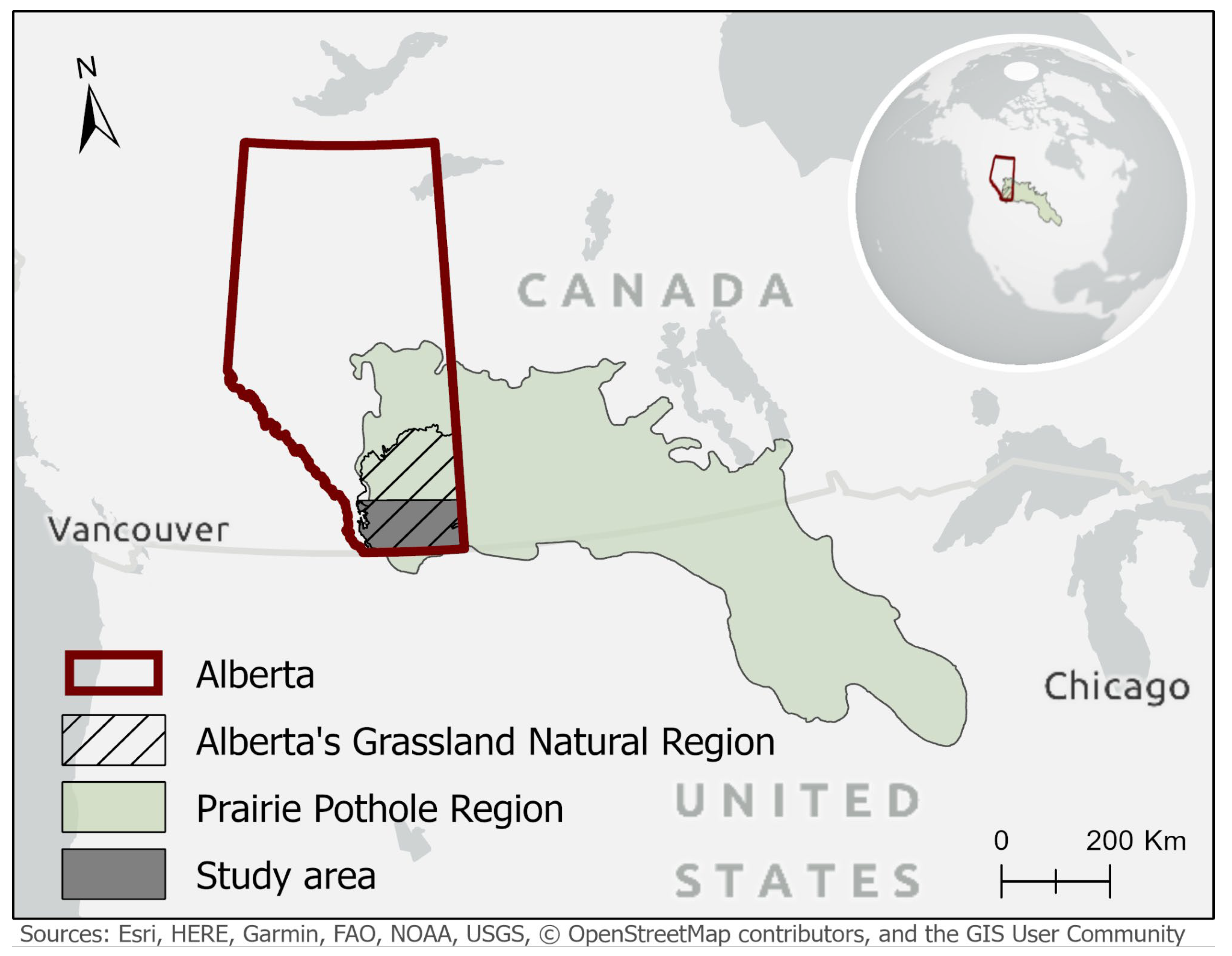
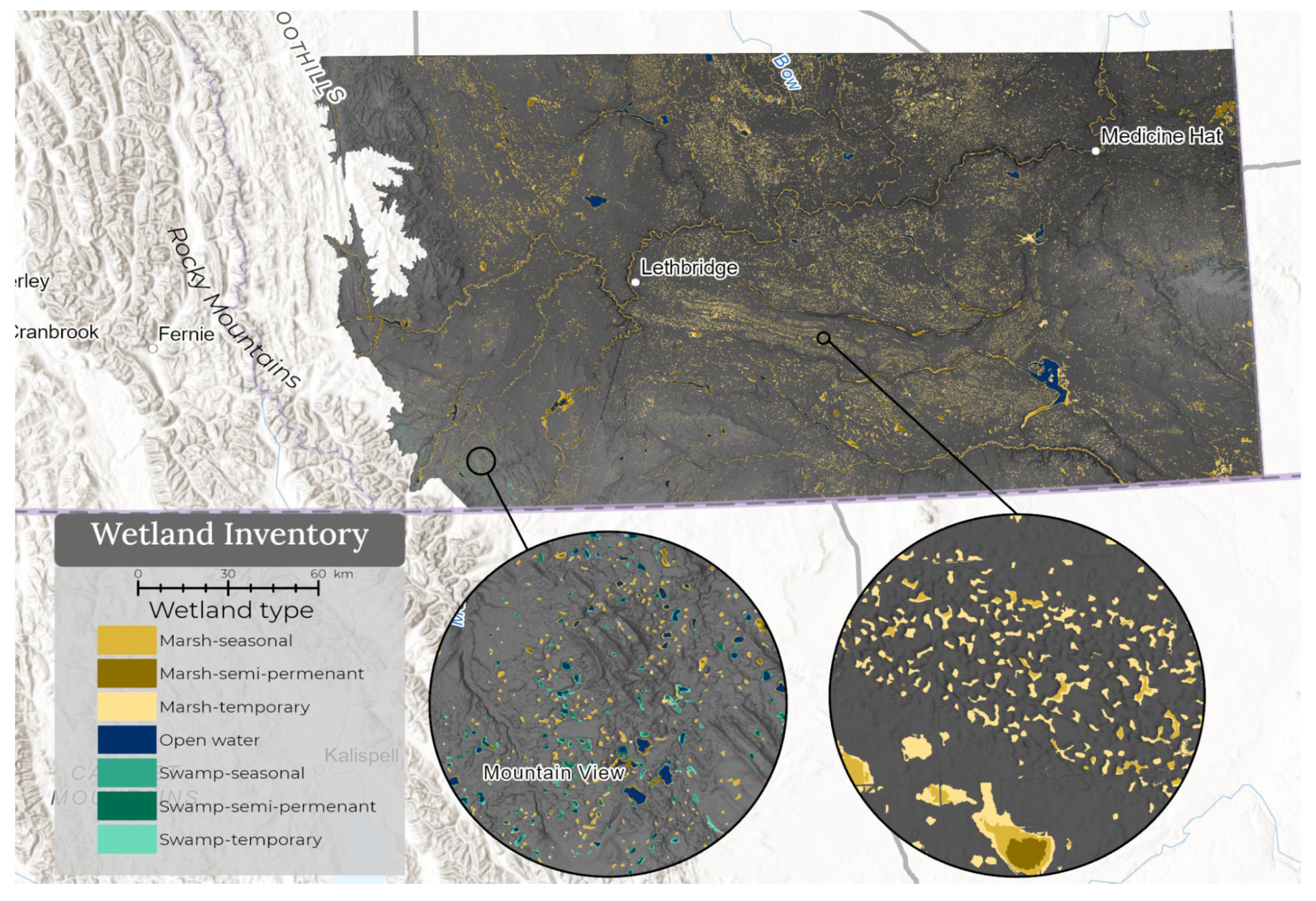
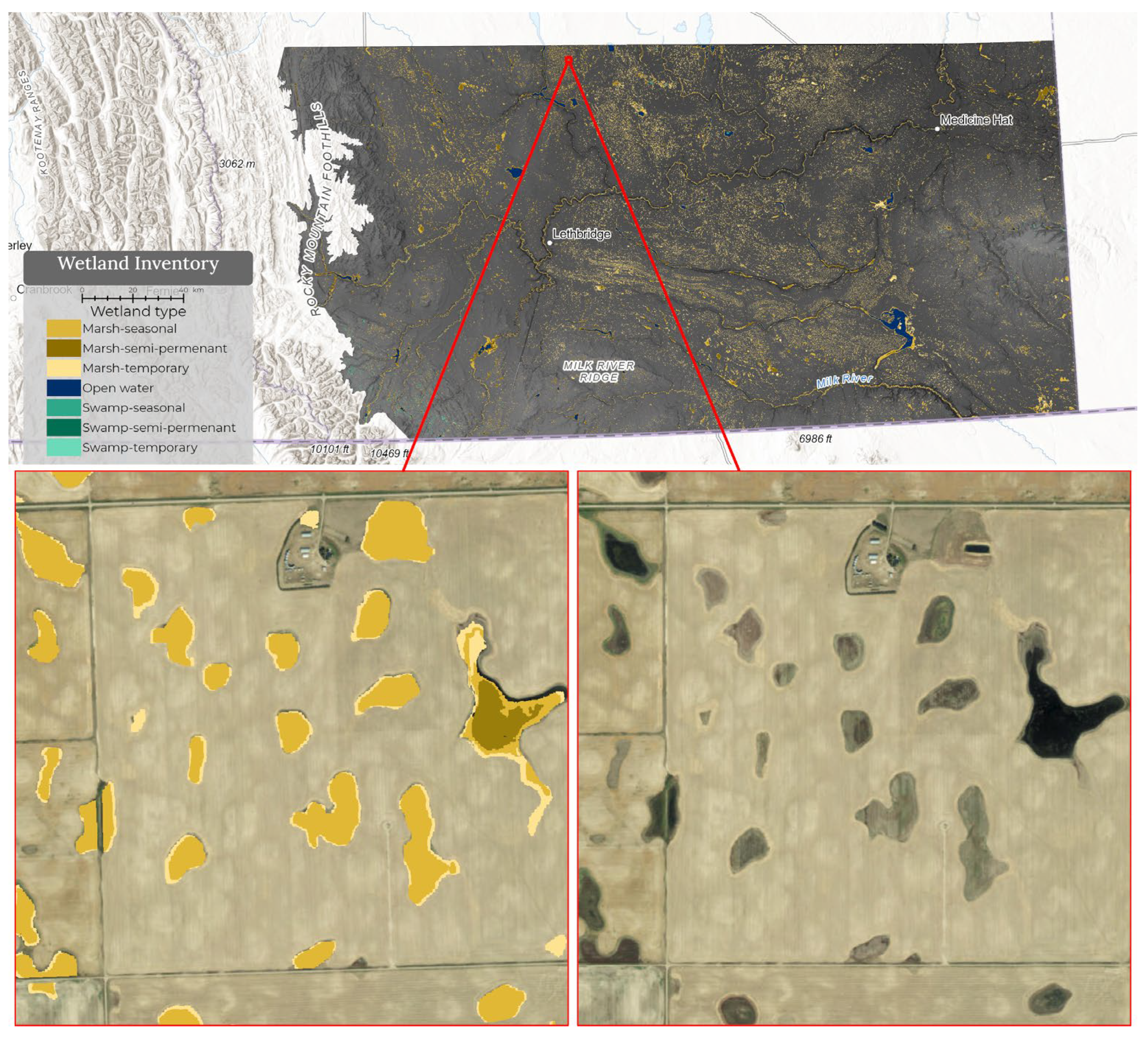
2.1. Study Area
2.2. Data
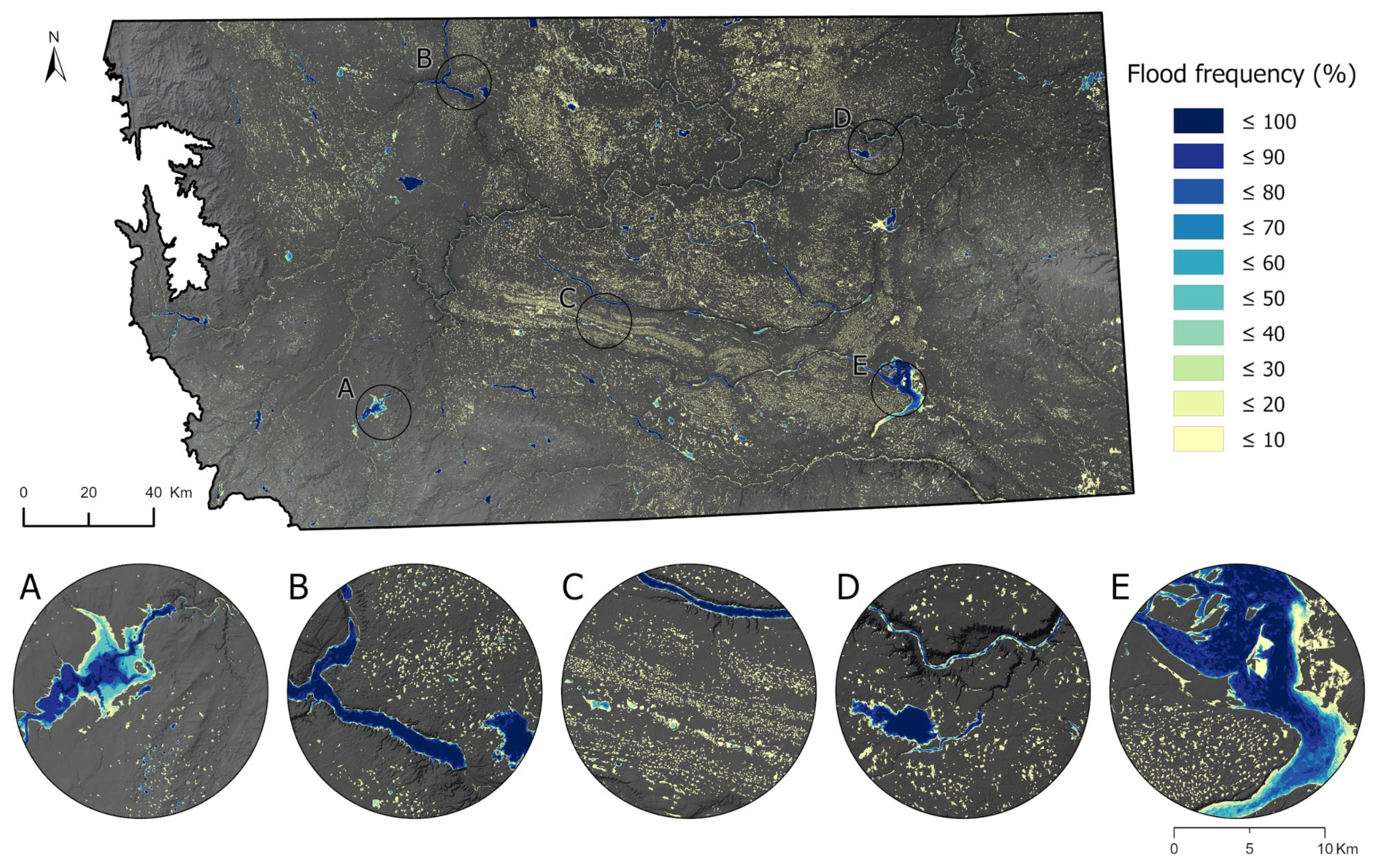
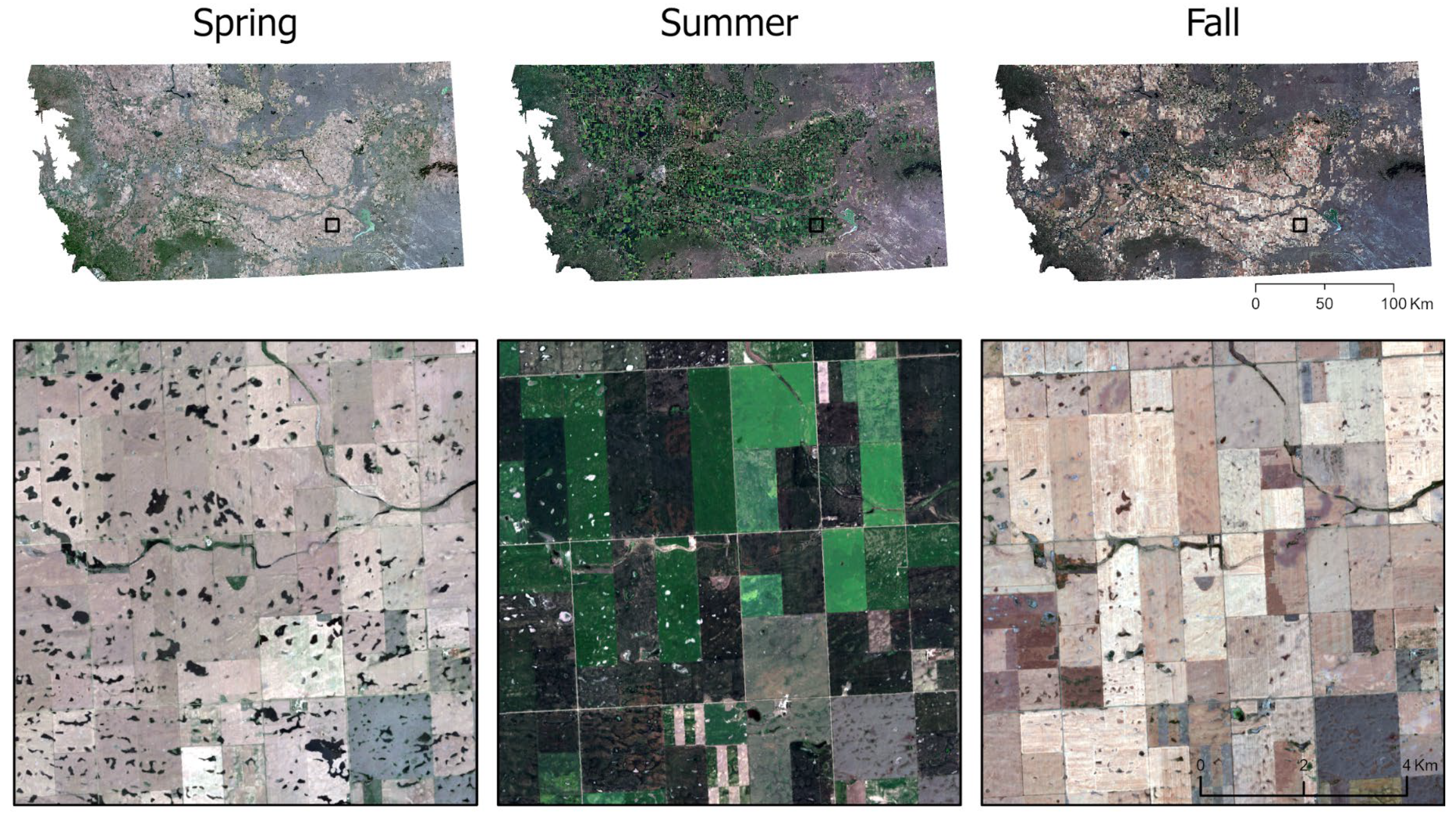
2.3. Hydroperiod
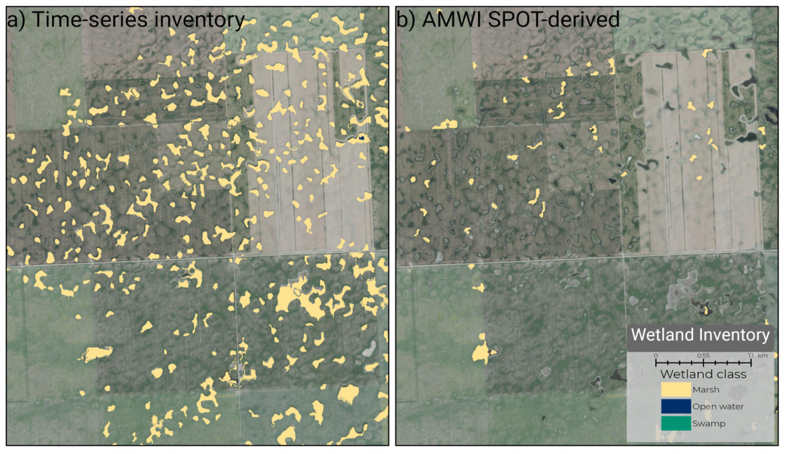
2.4. Wetland Inventory
2.5. Accuracy Assessment
3. Results
4. Discussion
5. Conclusions
Author Contributions
Funding
Data Availability Statement
Acknowledgments
Conflicts of Interest
References
- Batt, B.; Anderson, M.; Anderson, C.; Caswell, F. The Use of Prairie Potholes by North American Ducks. In Northern Prairie Wetlands; van der Valke, A., Ed.; Iowa State University Press: Ames, IA, USA, 1989; Volume 204, p. 227. [Google Scholar]
- Pattison-Williams, J.K.; Pomeroy, J.W.; Badiou, P.; Gabor, S. Wetlands, flood control and ecosystem services in the Smith Creek Drainage Basin: A case study in Saskatchewan, Canada. Ecol. Econ. 2018, 147, 36–47. [Google Scholar] [CrossRef]
- Wu, Q.; Lane, C.R. Delineation and quantification of wetland depressions in the Prairie Pothole Region of North Dakota. Wetlands 2016, 36, 215–227. [Google Scholar] [CrossRef]
- Wu, Q.; Lane, C.R.; Wang, L.; Vanderhoof, M.K.; Christensen, J.R.; Liu, H. Efficient delineation of nested depression hierarchy in digital elevation models for hydrological analysis using level-set method. J. Am. Water Resour. Assoc. 2019, 55, 354–368. [Google Scholar] [CrossRef] [PubMed]
- Dahl, T.E. Wetlands Losses in the United States, 1780’s to 1980’s; US Department of the Interior, Fish and Wildlife Service: Washington, DC, USA, 1990. [Google Scholar]
- Brinson, M.M.; Malvárez, A.I. Temperate freshwater wetlands: Types, status, and threats. Environ. Conserv. 2002, 28, 115–133. [Google Scholar] [CrossRef]
- Warner, B.; Rubec, C. The Canadian Wetland Classification System; Wetlands Research Centre, University of Waterloo: Waterloo, ON, Canada, 1997. [Google Scholar]
- Water Policy Branch, Policy and Planning Division. Alberta Environment and Sustainable Resource Development. In Alberta Wetland Classification System; Water Policy Branch, Policy and Planning Division: Edmonton, AB, Canada, 2015. [Google Scholar]
- Stewart, R.E.; Kantrud, H.A. Classification of Natural Ponds and Lakes in the Glaciated Prairie Region; U.S. Bureau of Sport Fisheries and Wildlife: Washington, DC, USA, 1971; Volume 92. [Google Scholar]
- Montgomery, J.S.; Mahoney, C.; Brisco, B.; Boychuk, L.; Cobbaert, D.; Hopkinson, C. Remote Sensing of Wetlands in the Prairie Pothole Region of North America. Remote Sens. 2021, 13, 3878. [Google Scholar] [CrossRef]
- Boudart, J. Mapping the Way for Conservation: Using Cutting-Edge Geographic Information Systems Technology, Ducks Unlimited Is Harnessing the Power of Data to Guide Its Work. Available online: https://www.ducks.org/conservation/national/mapping-the-way-for-conservation (accessed on 23 May 2022).
- Hird, J.N.; DeLancey, E.R.; McDermid, G.J.; Kariyeva, J. Google earth engine, open-access satellite data, and machine learning in support of large-area probabilistic wetland mapping. Remote Sens. 2017, 9, 1315. [Google Scholar] [CrossRef] [Green Version]
- Amani, M.; Mahdavi, S.; Afshar, M.; Brisco, B.; Huang, W.; Mirzadeh, S.M.J.; White, L.; Banks, S.; Montgomery, J.; Hopkinson, C. Canadian wetland inventory using google earth engine: The first map and preliminary results. Remote Sens. 2019, 11, 842. [Google Scholar] [CrossRef] [Green Version]
- Merchant, M.A.; Warren, R.K.; Edwards, R.; Kenyon, J.K. An object-based assessment of multi-wavelength SAR, optical imagery and topographical datasets for operational wetland mapping in boreal Yukon, Canada. Can. J. Remote Sens. 2019, 45, 308–332. [Google Scholar] [CrossRef]
- DeLancey, E.R.; Simms, J.F.; Mahdianpari, M.; Brisco, B.; Mahoney, C.; Kariyeva, J. Comparing deep learning and shallow learning for large-scale wetland classification in Alberta, Canada. Remote Sens. 2020, 12, 2. [Google Scholar] [CrossRef] [Green Version]
- Mahdianpari, M.; Salehi, B.; Mohammadimanesh, F.; Brisco, B.; Homayouni, S.; Gill, E.; DeLancey, E.R.; Bourgeau-Chavez, L. Big data for a big country: The first generation of Canadian wetland inventory map at a spatial resolution of 10-m using Sentinel-1 and Sentinel-2 data on the Google Earth Engine cloud computing platform. Can. J. Remote Sens. 2020, 46, 15–33. [Google Scholar] [CrossRef]
- DeVries, B.; Huang, C.; Lang, M.W.; Jones, J.W.; Huang, W.; Creed, I.F.; Carroll, M.L. Automated quantification of surface water inundation in wetlands using optical satellite imagery. Remote Sens. 2017, 9, 807. [Google Scholar] [CrossRef] [Green Version]
- Alberta Biodiversity Monitoring Institute. ABMI 3x7 Photoplot Landcover Dataset Data Model; Alberta Biodiversity Monitoring Institute: Edmonton, AB, Canada, 2016; p. 69. [Google Scholar]
- Castilla, G.; Hird, J.; Hall, R.J.; Schieck, J.; McDermid, G.J. Completion and updating of a landsat-based land cover polygon layer for Alberta, Canada. Can. J. Remote Sens. 2014, 40, 92–109. [Google Scholar] [CrossRef]
- DeLancey, E.R.; Kariyeva, J.; Bried, J.T.; Hird, J.N. Large-scale probabilistic identification of boreal peatlands using Google Earth Engine, open-access satellite data, and machine learning. PLoS ONE 2019, 14, e0218165. [Google Scholar] [CrossRef] [PubMed] [Green Version]
- Pouliot, D.; Latifovic, R.; Pasher, J.; Duffe, J. Assessment of convolution neural networks for wetland mapping with landsat in the central Canadian boreal forest region. Remote Sens. 2019, 11, 772. [Google Scholar] [CrossRef] [Green Version]
- Amani, M.; Brisco, B.; Mahdavi, S.; Ghorbanian, A.; Moghimi, A.; Delancey, E.; Merchant, M.A.; Jahncke, R.; Fedorchuk, L.; Mui, A. Evaluation of the Landsat-based Canadian Wetland Inventory Map using Multiple Sources: Challenges of Large-scale Wetland Classification using Remote Sensing. IEEE J. Sel. Top. Appl. Earth Obs. Remote Sens. 2020, 14, 32–52. [Google Scholar] [CrossRef]
- Amani, M.; Poncos, V.; Brisco, B.; Foroughnia, F.; DeLancey, E.D.; Ranjbar, S. InSAR Coherence Analysis for Wetlands in Alberta, Canada Using Time-Series Sentinel-1 Data. Remote Sens. 2021, 13, 3315. [Google Scholar] [CrossRef]
- Wu, Q.; Lane, C.R.; Li, X.; Zhao, K.; Zhou, Y.; Clinton, N.; DeVries, B.; Golden, H.E.; Lang, M.W. Integrating LiDAR data and multi-temporal aerial imagery to map wetland inundation dynamics using Google Earth Engine. Remote Sens. Environ. 2019, 228, 1–13. [Google Scholar] [CrossRef] [Green Version]
- Gorelick, N.; Hancher, M.; Dixon, M.; Ilyushchenko, S.; Thau, D.; Moore, R. Google Earth Engine: Planetary-scale geospatial analysis for everyone. Remote Sens. Environ. 2017, 202, 18–27. [Google Scholar] [CrossRef]
- Brisco, B.; Schmitt, A.; Murnaghan, K.; Kaya, S.; Roth, A. SAR polarimetric change detection for flooded vegetation. Int. J. Digit. Earth 2013, 6, 103–114. [Google Scholar] [CrossRef]
- Brisco, B. Mapping and Monitoring Surface Water and Wetlands with Synthetic Aperture radar. In Remote Sensing of Wetlands: Applications and Advances; Tiner, R.W., Lang, M.W., Klemas, V.V., Eds.; CRC Press, Taylor & Francis Group: Boca Raton, FL, USA, 2015; pp. 119–136. [Google Scholar]
- White, L.; Brisco, B.; Dabboor, M.; Schmitt, A.; Pratt, A. A collection of SAR methodologies for monitoring wetlands. Remote Sens. 2015, 7, 7615–7645. [Google Scholar] [CrossRef] [Green Version]
- DeLancey, E.R.; Kariyeva, J.; Cranston, J.; Brisco, B. Monitoring hydro temporal variability in Alberta, Canada with multi-temporal Sentinel-1 SAR data. Can. J. Remote Sens. 2018, 44, 1–10. [Google Scholar] [CrossRef]
- Schaffler, S.; Chini, M.; Dorigo, W.; Plank, S. Monitoring surface water dynamics in the Prairie Pothole Region of North Dakota using dual-polarised Sentinel-1 synthetic aperture radar (SAR) time series. Hydrol. Earth Syst. Sci. 2022, 26, 841–860. [Google Scholar] [CrossRef]
- Montgomery, J.S.; Hopkinson, C.; Brisco, B.; Patterson, S.; Rood, S.B. Wetland hydroperiod classification in the western prairies using multitemporal synthetic aperture radar. Hydrol. Process. 2018, 32, 1476–1490. [Google Scholar] [CrossRef]
- DeLancey, E.R.; Brisco, B.; Canisius, F.; Murnaghan, K.; Beaudette, L.; Kariyeva, J. The synergistic use of RADARSAT-2 ascending and descending images to improve surface water detection accuracy in Alberta, Canada. Can. J. Remote Sens. 2019, 45, 759–769. [Google Scholar] [CrossRef]
- Natural Regions Committee. Natural Regions and Subregions of Alberta; Downing, D.J., Pettapiece, W.W., Eds.; Government of Alberta: Edmonton, AB, Canada, 2006. [Google Scholar]
- Environment Canada. Medicine Hat Historical Weather. Available online: https://climate.weather.gc.ca/historical_data/search_historic_data_e.html (accessed on 18 May 2021).
- Winter, T.C.; Rosenberry, D.O. The interaction of ground water with prairie pothole wetlands in the Cottonwood Lake area, east-central North Dakota, 1979–1990. Wetlands 1995, 15, 193–211. [Google Scholar] [CrossRef]
- Huang, S.; Dahal, D.; Young, C.; Changder, G.; Liu, S. Integration of Palmer Drought Severity Index and remote sensing data to simulate wetland water surface from 1910 to 2009 in Cottonwood Lake area, North Dakota. Remote Sens. Environ. 2011, 115, 337–3389. [Google Scholar] [CrossRef] [Green Version]
- Alberta Biodiversity Monitoring Institute and Alberta Human Footprint Monitoring Program. Alberta Biodiversity Monitoring Institute and Alberta Human Footprint Monitoring Program Wall-to-Wall Human Footprint Inventory 2018; Alberta Biodiversity Monitoring Institute and Alberta Human Footprint Monitoring Program: Edmonton, AB, Canada, 2020; p. 145. [Google Scholar]
- Esri. “Light Gray Canvas” [Baselayer]. Scale not Given. Created: 26 September 2011. Available online: https://www.arcgis.com/home/item.html?id=8b3d38c0819547faa83f7b7aca80bd76 (accessed on 23 May 2022).
- Potapov, P.; Li, X.; Hernandez-Serna, A.; Tyukavina, A.; Hansen, M.C.; Kommareddy, A.; Pickens, A.; Turubanova, S.; Tang, H.; Silva, C.E. Mapping global forest canopy height through integration of GEDI and Landsat data. Remote Sens. Environ. 2021, 253, 112165. [Google Scholar] [CrossRef]
- Achanta, R.; Susstrunk, S. Superpixels and Polygons Using Simple Non-Iterative Clustering. In Proceedings of the IEEE Conference on Computer Vision and Pattern Recognition, Honolulu, HI, USA, 21–25 July 2017. [Google Scholar]
- Breiman, L.; Friedman, J.; Stone, C.J.; Olshen, R.A. Classification and Regression Trees; Routeledge: New York, NY, USA, 1984; p. 368. [Google Scholar] [CrossRef]
- Esri. “Terrain with Labels” [Baselayer]. Scale not Given. Created: 9 June 2016. Available online: https://www.arcgis.com/home/item.html?id=a52ab98763904006aa382d90e906fdd5 (accessed on 23 May 2022).
- Esri. “World Imagery” [Baselayer]. Scale not Given. Created: 12 December 2009. Available online: https://www.arcgis.com/home/item.html?id=10df2279f9684e4a9f6a7f08febac2a9 (accessed on 23 May 2022).
- Hardy, A.; Oakes, G.; Ettritch, G. Tropical Wetland (TropWet) Mapping Tool: The Automatic Detection of Open and Vegetated Waterbodies in Google Earth Engine for Tropical Wetlands. Remote Sens. 2020, 12, 1182. [Google Scholar] [CrossRef] [Green Version]
- Pekel, J.-F.; Cottam, A.; Gorelick, N.; Belward, A.S. High-resolution mapping of global surface water and its long-term changes. Nature 2016, 540, 418–422. [Google Scholar] [CrossRef]
- ABMI Wetland Inventory. Available online: https://abmi.ca/home/data-analytics/da-top/da-product-overview/Advanced-Landcover-Prediction-and-Habitat-Assessment--ALPHA--Products/ABMI-Wetland-Inventory.html (accessed on 23 May 2022).


| Class | Forms | Water Permanence Types 1 |
|---|---|---|
| Marsh | Graminoid | Temporary [II] |
| Seasonal [III] | ||
| Semi-permanent [IV] | ||
| Swamp | Wooded, coniferous | |
| Wooded, mixedwood | ||
| Wooded, deciduous | ||
| Shrubby | Temporary [II] 2 | |
| Seasonal [III] 2 | ||
| Shallow Open Water | Subersed and/or floating aquatic vegetation | Seasonal [III] |
| Semi-permanent [IV] | ||
| Permanent [V] | ||
| Intermittent [VI] | ||
| Bare | Seasonal [III] | |
| Semi-permanent [IV] | ||
| Permanent [V] | ||
| 1 Roman numerals for wetland permanence types relate to wetland classes as outlined in [9]. | ||
| 2 Swamp water permanence types are only applicable to shrubby swamps given a current a lack of available information on wooded swamp types. | ||
| Hydroperiod Value (%) | Vegetation Height (m) | Wetland Classification |
|---|---|---|
| 85–100 | Not applied | Open water |
| 51–84 | <2 | Semi-permanent marsh |
| 51–84 | >2 | Semi-permanent swamp |
| 20–50 | <2 | Seasonal marsh |
| 20–50 | >2 | Seasonal swamp |
| 1–19 | <2 | Temporary marsh |
| 1–19 | >2 | Temporary swamp |
| 0–1 | Not applied | Upland |
| Hydroperiod-Based Wetland Inventory | ||||||
|---|---|---|---|---|---|---|
| Validation Dataset | Marsh | Open Water | Swamp | Upland | Total | Producer Accuracy |
| Marsh | 2260.33 | 0.04 | 0.58 | 878 | 3138.95 | 0.72 |
| Shallow Open water | 616.24 | 66.67 | 1.19 | 42.31 | 726.41 | 0.09 |
| Swamp | 0.1 | 0.1 | ||||
| Upland | 903.62 | 0.09 | 45,225.74 | 46,129.45 | 0.98 | |
| Total | 3780.19 | 66.71 | 1.86 | 46,146.15 | ||
| User Accuracy | 0.6 | 1 | 0.98 | OA = 95% | ||
| Hydroperiod-Based Wetland Inventory | ||||
|---|---|---|---|---|
| Validation Dataset | Wetland | Upland | Total | Producer Accuracy |
| Wetland | 2945.05 | 920.41 | 3865.46 | 0.76 |
| Upland | 903.71 | 45,225.74 | 46,129.45 | 0.98 |
| Total | 3848.76 | 46,146.15 | ||
| User Accuracy | 0.77 | 0.98 | OA = 96% | |
Publisher’s Note: MDPI stays neutral with regard to jurisdictional claims in published maps and institutional affiliations. |
© 2022 by the authors. Licensee MDPI, Basel, Switzerland. This article is an open access article distributed under the terms and conditions of the Creative Commons Attribution (CC BY) license (https://creativecommons.org/licenses/by/4.0/).
Share and Cite
DeLancey, E.R.; Czekajlo, A.; Boychuk, L.; Gregory, F.; Amani, M.; Brisco, B.; Kariyeva, J.; Hird, J.N. Creating a Detailed Wetland Inventory with Sentinel-2 Time-Series Data and Google Earth Engine in the Prairie Pothole Region of Canada. Remote Sens. 2022, 14, 3401. https://doi.org/10.3390/rs14143401
DeLancey ER, Czekajlo A, Boychuk L, Gregory F, Amani M, Brisco B, Kariyeva J, Hird JN. Creating a Detailed Wetland Inventory with Sentinel-2 Time-Series Data and Google Earth Engine in the Prairie Pothole Region of Canada. Remote Sensing. 2022; 14(14):3401. https://doi.org/10.3390/rs14143401
Chicago/Turabian StyleDeLancey, Evan R., Agatha Czekajlo, Lyle Boychuk, Fiona Gregory, Meisam Amani, Brian Brisco, Jahan Kariyeva, and Jennifer N. Hird. 2022. "Creating a Detailed Wetland Inventory with Sentinel-2 Time-Series Data and Google Earth Engine in the Prairie Pothole Region of Canada" Remote Sensing 14, no. 14: 3401. https://doi.org/10.3390/rs14143401