
High Wind Geophysical Model Function Modeling for the HY-2A Scatterometer Using Neural Network


1
School of Geography and Remote Sensing, Guangzhou University, Guangzhou 510006, China
2
School of Geography and Planning, Sun Yat-sen University, Guangzhou 510275, China
3
National Satellite Ocean Application Service, Beijing 100081, China
*
Author to whom correspondence should be addressed.
Remote Sens. 2022, 14(10), 2335; https://doi.org/10.3390/rs14102335
Submission received: 2 March 2022
/
Revised: 2 May 2022
/
Accepted: 10 May 2022
/
Published: 12 May 2022
(This article belongs to the Special Issue High Winds and High Seas)
Abstract
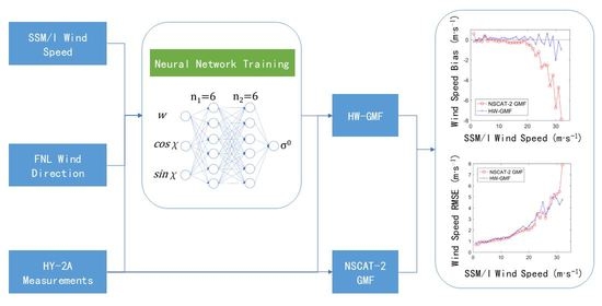
:Under low to medium wind speeds and no rainfall, the retrieved vector wind from a scatterometer is accurate and reliable. However, under high wind conditions, the currently used geophysical model function (GMF), such as NSCAT-2, for wind vector retrieval has the disadvantage of overestimating the backscattering coefficient, which leads to a decrease in the quality of the retrieved ocean surface winds. To enhance the wind retrieval precision of the HY-2A scatterometer under high wind conditions, a new GMF for high wind (HW-GMF) is established by using the neural network method based on the backscattering coefficient data of the HY-2A scatterometer combined with the wind speed data of the Special Sensor Microwave Imager (SSM/I) and the Final (FNL) operational global analysis wind direction data from the National Centers for Environmental Prediction (NCEP). The absolute value of the mean deviation between the predicted σ0 by the HW-GMF and the measured σ0 by the HY-2A scatterometer is less than 0.1 dB, indicating that the HW-GMF has high accuracy. To verify the HW-GMF performance, the wind field inversion accuracy of the HW-GMF is compared with that of the NSCAT-2 GMF, a GMF currently used in the data processing of the HY-2A scatterometer. The experimental results show that the deviation between the HW-GMF retrieved wind speed and the SSM/I wind speed is within 2 m/s in the high wind speed range of 15–35 m/s, indicating that the HW-GMF improves the precision of the wind speed inversion of the HY-2A scatterometer under high wind speed conditions.
1. Introduction
The sea surface wind stress is the largest source of momentum that directly drives the movement of seawater at various scales, which ranges from sea surface waves to the ocean current system. The sea surface wind couples the atmosphere and the ocean and regulates the global and regional climate by promoting the exchange of heat, water, and chemicals between the atmosphere and the ocean. Knowledge of the ocean wind is the basis for understanding the principles and mechanisms of many oceanic, meteorological, and climatic phenomena, and this information also plays a vital role in predicting changes in air-sea interactions [1]. Therefore, the ocean surface wind observation data can be used in regional and global numerical weather prediction systems to expand forecast capability and improve forecast accuracy of future weather at different scales.
Before microwave radars were widely used, the ocean surface wind observation was generally performed by traditional methods, and the platforms equipped with the anemometer mainly include ships, offshore buoys, and coastal stations. Sea surface wind observation data based on buoy or ship measurements have high accuracy at low and medium wind speeds, but these real-time wind measurement devices can only observe the wind vector at a particular point, and the spatial and temporal distribution is uneven and cannot cover the global ocean [2]. After the introduction of microwave radar observation methods, the satellite microwave scatterometer was proven to be one of the effective instruments that is capable of measuring the ocean surface wind speed and direction simultaneously, under almost all weather conditions. Seasat-A was the first marine satellite launched by the National Aeronautics and Space Administration (NASA) in 1978, and it was equipped with a Ku-band scatterometer. In the study of the Seasat-A scatterometer, it was found that under the conditions of moderate wind speeds, the retrieved wind vectors were consistent with the instrument design specifications, which demonstrates that the Ku-band scatterometer has a high feasibility for measuring the sea surface wind field with moderate wind speeds [3,4]. In contrast, the scatterometer series developed by the European Space Agency (ESA) are the C-band spaceborne microwave instruments. The first operational C-band scatterometer was carried onboard the European Remote Sensing (ERS) satellite ERS-1. Quilfen and Bentamy tested the accuracy of the wind field product of the ERS-1 scatterometer and found that the wind inversion accuracy of the ERS-1 scatterometer was reliable except for in the case of a low incidence angle [5]. Early Ku-band and C-band scatterometers have been testified to be effective sensors for ocean surface wind observation.
Relying on the data obtained in the laboratory, many researchers have conducted theoretical studies on the relationship between the wind and backscattering coefficients [6]. Due to the complexity of the interaction between the ocean surface and microwave, these geophysical model functions (GMFs) based on theoretical research cannot be fully applied to operational wind field inversion [7]. Therefore, at present, a GMF based on empirical fitting is usually used in the operational wind vector inversion of a scatterometer [8,9,10,11,12,13]. By comparing the normalized radar cross section (NRCS) measured by the airborne C/Ku band scatterometer and the NRCS predicted by COMD4, SASS 2, and NSCAT-1, Carswell et al. found that all three GMFs overestimate the backscatter coefficients to some extent compared with the measured NRCS when the wind speed exceeds 15 m/s [14,15]. In addition to research on the measurement accuracy of airborne scatterometers under high wind speed conditions, researchers have also studied the performance of spaceborne scatterometers in high wind speed range. Because the synchronous observation data under different conditions is limited, there are fewer on-site verification data for spaceborne scatterometers. However, the research results show that the spaceborne scatterometer has the same trend as the airborne scatterometer in the inversion of the wind field; that is, under high wind conditions, the wind inversion precision by the scatterometer in Ku band and C band decreases. In the study of satellite ERS-1, Zeng and Brown pointed out that due to the errors in the buoy data or numerical weather prediction wind data used for modelling and verifying the GMF, for wind speeds greater than 20 m/s, the error inherited from the buoy data or numerical model wind data causes the retrieved wind speed by the ERS-1 scatterometer to be underestimated relative to its actual value [16]. In strong wind conditions, the NRCS measured by the scatterometer still contains wind speed information. Zec and Jones found that when the wind speed does not exceed 15 m/s, that is, under the moderate wind speed conditions, the wind retrieval accuracy of NSCAT is reliable, but when the wind speed exceeds 20 m/s, the NSCAT scatterometer underestimates the retrieved wind speed. To solve this problem, a specific GMF for tropical cyclone wind retrieval (TCGMF) was established to improve the precision of high wind speed inversion of NSCAT [17]. Yueh et al. studied and verified the performance of the QuikSCAT scatterometer in the wind inversion of typhoon Floyd. The results showed that the NSCAT-2 GMF used in wind field inversion causes the inverted wind speed to be underestimated. To solve this problem in the NSCAT-2 GMF, they proposed an improved GMF that can enhance the performance of the QuikSCAT scatterometer for typhoon wind observation [18]. In the follow-up study, Yueh et al. improved the second harmonic coefficient A2 of the QSCAT1 GMF representing the ratio of the backscatter coefficient under the conditions of upwind and crosswind and proposed a GMF, which can be used for wind field inversion with wind speeds above 23 m/s. The results show that the proposed GMF is effective for improving the wind inversion precision under the condition of high wind speeds [19].
In summary, ocean surface wind inversion under strong wind conditions by a scatterometer has already been one of the difficult problems in scatterometry. The reasons for the decline of high wind speed inversion precision of a scatterometer may include the following aspects:
- (1)
- Declined sensitivity in backscatter
Relevant studies have shown that C and Ku-band scatterometers both have the problem of a reduced sensitivity in the backscattering coefficients for the wind speeds above 30 m/s. For C-band, when wind speed is above 35 m/s, the backscattering coefficient starts to become saturated, which means that different wind speeds may produce very similar backscattering coefficients, which will eventually lead to a degradation of wind inversion precision.
- (2)
- Rain effect
Strong winds and rain often accompany each other. Rainfall has a direct impact on backscatter measurement of scatterometer, by backscattering the forward signal from the rain-droplets, and by attenuating the returned signal. Rainfall also impacts the observations that are often used as inputs for building a GMF, resulting in a bad GMF at high winds. Therefore, very strict rain flagging of these observations has to be performed in wind retrieval.
- (3)
- Scarcity of observations
There is a scarcity of observations at very high winds to use as ground truth to develop the GMFs. GMFs based on empirical methods are usually obtained by statistical fitting of the sea surface backscattering coefficients and the synchronously measured sea surface wind field or numerical forecast wind field. Because there are few data samples with high wind speeds on the sea surface, most of the GMF curves for high wind speed segments are constructed by empirical extrapolation, which usually results in the underestimation of the wind speeds retrieved by these GMFs in high wind speed conditions. Moreover, the noise due to the scarcity of observations results in wrong estimates of the GMF coefficients.
The HY-2A scatterometer was put into operation in October 2011, which adopts dual-polarized pencil beam, conical scanning mode, and works in Ku band with a center frequency of 13.256 GHz. The scatterometer makes observations from two incident angles with two polarizations: the inner beam corresponds to HH polarization, and the outer beam corresponds to VV polarization, and the incident angles are 41° and 48°, respectively, which can provide a global ocean wind observation at a spatial resolution of 25 km. The NSCAT-2 model is currently used to retrieve ocean surface wind from the HY-2A scatterometer measurements [20]. Since the launch of the HY-2A satellite, many scholars have evaluated or improved the wind measurement accuracy of its scatterometer. In their study of the HY-2A scatterometer radiometric calibration, Mu and Song considered that GMF has a great influence on the calibration process. It is found that there is some systematic deviation among different GMFs when using an ocean target method for radiometric calibration [21]. Using the ocean target calibration technique, Peng et al. found that the calibration coefficient of the HY-2A scatterometer NRCS is 1.7 dB for both VV and HH polarizations, and they further verified the stability and reliability of the scatterometer measurement by the Amazon rainforest. Accordingly, the RMS errors of the retrieved wind speed and direction are approximately 1.19 m/s and 18.74°, respectively [22]. Wang et al. validated the wind inversion precision of the HY-2A scatterometer by comparing the retrieved winds with the collocated International Comprehensive Ocean-Atmosphere Data Set (ICOADS), and found that in conditions of medium and low wind speed, HY-2A wind speed is similar to ICOADS wind speed, while in high wind speed conditions, the HY-2A scatterometer tends to underestimate the wind speed [23]. Xing et al. verified the retrieved wind field data of HY-2A scatterometer during 2012 to 2014 by using buoy data, ECMWF wind field data, and ASCAT scatterometer wind data. It was found that the RMSE error of wind speed was less than 2 m/s in the range of 2–24 m/s, which could meet the designed quality requirement [24]. Wang et al. conducted a first quality assessment of HY-2A SCAT wind products through the comparison of the first six months operationally released SCAT wind products with in situ data and found that HY-2A wind speed has an increased negative bias with increasing wind speed above 3 m/s compared against oceanic buoy data [25]. Wu and Chen made a validation and intercomparison HY-2A, Metop-A, and Oceansat-2 scatterometers based on buoy wind data and concluded that the HY-2A scatterometer nearly meets the mission requirement with RMSE 1.23 m/s for wind speed and 22.85° for wind direction and no seasonal variation was found [26]. Yang et al. found that the wind speed residuals of HY-2A are higher in low and high wind speed ranges than in moderate wind speeds when compared with in situ observations [27]. Zheng et al. demonstrated that both bias and RMSE of wind speeds between HY-2A and WindSat show latitude dependence and have significant latitudinal fluctuations [28]. Xu et al. proposed an artificial neural network to retrieve wind field by combining the observations of the radiometer and scatterometer onboard the HY-2A satellite and obtained a better result than using scatterometer data alone [29]. Xie et al. attempted to build a rain effect correction model based on neural network for the HY-2A scatterometer in rainy conditions and found that the neural network can effectively reduce systematic deviation in backscatter coefficients as well as in the retrieved wind speed caused by rain [30]. Zhang et al. made an evaluation of the performance of HY-2B scatterometer with the Amazon Forest observations and found that the scatterometer instrument had met all the design requirements [31]. Wang et al. validated the wind products of the HY-2C scatterometer by comparing them to collocated buoys and ECMWF winds and showed that the HY-2C winds have a good agreement with the HY-2B winds in the wind speed range of 4–17 m/s [32].
The NSCAT-2 GMF is a semiempirical model based on numerical weather prediction (NWP) wind data. Due to the scarcity of NWP wind data in high wind speed range, the NSCAT-2 model is established by the extrapolation method when the wind speed is above 20 m/s [18]. Therefore, the ocean surface wind vector values retrieved by this GMF also have poor wind speed accuracy under strong wind conditions. To improve the HY-2A scatterometer accuracy in wind measurement under strong wind conditions, the SSM/I wind speed data and the FNL wind direction data are collocated and used to establish a neural network-based high wind speed GMF based on its observation characteristics in this paper. The novelty of this paper is to refine the geophysical model function of an HY-2A scatterometer at high wind speed by using a neural network.
This paper is organized as follows. The datasets, data validation, and the methods of GMF modeling and wind vector retrieval are introduced in Section 2. The experimental results as well as some preliminary explanations and analysis are described in detail in Section 3. Section 4 and Section 5 present the discussion and conclusions, respectively.
2. Data and Methods
In this section, first, the HY-2A scatterometer backscattering coefficient data, SSM/I sea surface wind field data, FNL sea surface wind field data, TAO buoy measurement wind vector data, and NII typhoon data for GMF modeling are briefly described; then, the accuracy of SSM/I data and FNL data used to establish the GMF are validated; finally, the BP neural network for modelling the HW-GMF and the wind vector retrieval method by scatterometer are presented.
2.1. DataSet
2.1.1. HY-2A Scatterometer Data
One of the data sets used in this study is the level 2A data product of the HY-2A scatterometer with temporal coverage from 1 January 2013 to 31 December 2013. The parameters of the data product include the acquisition time of each measurement of the HY-2A scatterometer, the longitude and latitude of the center of each beam footprint, angle of incidence, observation azimuth, backscatter coefficient (σ0), and quality flag. Eight months of the data are used for modeling and four months for verification. The data set is divided into two parts according to the polarization mode; one corresponds to the VV polarization, and the other corresponds to the HH polarization. The unit of σ0 is the decibel unit (dB).
2.1.2. SSM/I Wind Field Data
The Special Sensor Microwave Imager (SSM/I) is a spaceborne microwave radiometer. Since 1987, the near polar orbit Defense Meteorological Satellite Program (DMSP) has been equipped with the SSM/I series radiometers. The SSM/I sensor contains seven microwave radiation channels that can be used to measure the microwave radiation from both the ground and atmosphere at the same time. According to the obtained microwave radiation, the radiant brightness temperature of the atmosphere, and that of the sea or land surface, can be estimated. The main parameters observed by the radiometer include the sea surface wind speed, sea surface temperature, water vapor in the atmosphere, liquid water in clouds, and rain rate.
In this study, the SSM/I data used in modeling and validation are from the remote sensing systems (RSS) website. The SSM/I data of RSS are generated by using a constantly improved inversion algorithm. For the SSMI radiometer, a radiative transfer model (RTM) is used to retrieve the ocean and atmosphere parameters. The general RTM function expression for a radiometer measurement can be written as follows [33]:
In the above formula, TB represents the brightness temperature measured by the radiometer, p denotes the polarization, TBU is the brightness temperature of the upward radiation from the atmosphere, τ is the transmittance of the atmosphere, Ep is the total emissivity of the ocean surface, TS denotes the sea surface temperature (SST), TBΩ is the brightness temperature of the downward sky radiation scattered by the ocean surface, Rp is the reflectivity of the ocean surface, TBD is the brightness temperature of the downward atmospheric radiation reflected by the ocean surface, Tcold is the effective brightness temperature of the cold space, and TB,scat,p is the atmospheric path length correction term for the downward radiation of the sky.
The emissivity of the ocean surface E can be expressed as the sum of the following three parts:
where E0 is the specular component of the ocean surface emissivity, ΔEW is the isotropic component induced by wind, and ΔEϕ is the wind direction-related emissivity component.
The algorithm has been refined, improved, and verified for more than 20 years and has high reliability. This study uses version 7 of the SSM/I data for modeling and verification. The SSM/I data are organized in the form of regular global latitude and longitude grids divided by 0.25 degrees, including the neutral wind speed at 10 m height above the ocean surface, water vapor in the atmosphere, liquid water in clouds, and rain rate, with a time interval of 0.2 h. This study uses the wind speed data of the SSM/I radiometer as one of the inputs to establish the high wind speed GMF for the HY-2A scatterometer. Because the SSM/I radiometer can only provide wind speed data, wind direction information from other data sources will be used in GMF modeling.
2.1.3. FNL Data
This study uses the FNL wind data from NCEP for GMF modeling. The FNL data are a global meteorological forecast data set generated by the Global Data Assimilation System (GDAS). Its time resolution and spatial resolution are 6 h and 1° × 1°, respectively. It provides various meteorological parameters, such as sea level pressure, sea surface temperature, ice cover, relative humidity, ocean surface wind (u and v components), and ozone. This study uses u and v components of the FNL 10 m neutral wind to derive wind direction for GMF modeling. The main reason why the FNL wind speed is not used for modeling is that, when compared with NII wind data at high wind speeds, the FNL wind speed is systematically lower. The detailed validation information is presented in Section 2.2.
2.1.4. TAO Data
The measurement wind data from 27 TAO buoys are used for wind quality verification. The measurement data of the TAO buoys, which are deployed and maintained by the National Data Buoy Center (NDBC) can provide various types of oceanic and atmospheric parameters, such as shortwave radiation, longwave radiation, rain rate, ocean surface vector wind (wind speed and direction), relative humidity, temperature of the air, sea surface pressure, sea surface temperature, temperature, salinity, and density of sea water. Most of the ocean surface wind vector data of TAO buoys are measured at a height of 4 m above the sea surface. Therefore, the wind speed measured at a height of 4 m must be converted to that at a height of 10 m, which is the reference height of the SSM/I and FNL data. The conversion formula is as follows [34,35]:
where Uz is the wind speed at a height of z, m, and u* denotes the friction velocity such that
where UN10 is the neutral wind speed at 10 m height; a and b are constant coefficients. In Equation (4), for UN10 < 8 m/s, a = 0.0283, b = 0.00513 m/s; and for UN10 ≥ 8 m/s, a = 0.051, b = −0.14 m/s [36,37]. The UN10 can be calculated by following equation:
where z0 is the roughness length, and k is the von Karman constant, which is usually assigned a value of 0.4 in practical applications. Using the Equations (3)–(5), the neutral stability winds at 10 m height, U10, can be accurately computed through an iterative process.
2.1.5. NII Typhoon Data
The NII typhoon historical data provided by UNISYS Weather are the reanalysis data after assimilation based on the National Oceanic and Atmospheric Administration (NOAA) marine meteorological observation data. The NII typhoon data provide the position and maximum wind speed of each typhoon moving center that occurs in the Atlantic, Pacific, and Indian Oceans every year. The accuracy of the wind speed is 5 knots (about 2.57 m/s), and the time frequency of acquisition is every 6 h.
2.2. Data Validation
This study is aimed at establishing a high wind GMF for the HY-2A scatterometer. Building such a GMF requires accurate external reference data for modeling and validation. To ensure the accuracy of the established GMF, there are certain requirements for the data volume. The TAO buoy data and the NII typhoon data described in the previous section are reliable in accuracy, but the amount of data is small, so it cannot be used as the reference data to construct the GMF. Therefore, in this study, these two kinds of data are used as validation data to evaluate the precision of the modeling data and to ensure the accuracy of high wind speed data used for modeling. Based on the above modeling data requirements, the authors use SSM/I and FNL data as inputs to establish the high wind speed GMF and use the TAO and NII data to verify the accuracy of these two data directly or indirectly.
First, the authors should evaluate the accuracy of the FNL wind data to determine whether it can meet the requirements of building a high wind speed GMF for the HY-2A scatterometer. The adopted method matches the FNL wind field data with the Tao buoy data in time and space and performs a statistical analysis on the errors. FNL data provide global gridded wind data of 1° × 1° every 6 h. The measurement interval of the TAO buoy data is 10 min, and the positions of the TAO buoys are distributed near the equator. FNL data and TAO data can be completely matched in time and space during the matching process. After matching the data from January to December 2013, a total of 18,766 match-up pairs of FNL and TAO spatiotemporal synchronous data were obtained, and the error of the FNL wind direction data was statistically analyzed.
When performing error statistics on the matched wind directions, the 360-degree periodicity of the wind direction data must be considered [38]. The numerical jump from 360° to 0° will lead to a discrepancy between the calculation result and its real value. Therefore, the wind direction deviation must be converted to a value between −180° and 180°. The conversion formula is as follows:
where dirFNL is the FNL wind direction, dirTAO is the TAO wind direction, and direr is the wind direction deviation between TAO and FNL (FNL wind direction minus the TAO wind direction). After a statistical calculation of the error, the average wind direction error of TAO and FNL is −0.3433°, and the root mean square error (RMSE) is 11.0203°. The statistical results show that the FNL wind direction and TAO wind direction have high fitting degrees and that the FNL wind direction has high accuracy. Figure 1a is a scatter plot between FNL and TAO matched wind direction data pairs. The wind direction trend reflected in the scatter plot is consistent with the statistical results. The scatter distribution of the FNL and TAO wind directions is concentrated, which shows that the difference between them is small.
This study used SSM/I wind speed and FNL wind direction as inputs for GMF modeling. The main reason for choosing SSM/I wind speed instead of FNL wind speed in modeling is that the FNL wind speed is lower than its corresponding real value under high wind conditions. To ensure the reliability of the GMF, the SSM/I wind speed data with higher accuracy should be used in modeling.
The data of wind speed retrieved by SSM/I and provided by RSS are obtained from the inversion of the sea surface brightness temperature model established by Wentz [39]. With the aid of the in situ data, the model has been continuously adjusted and improved through changes in the radiometer instrument parameters [40]. The retrieved sea surface wind speed has high accuracy and reliability. In the operational inversion model of the radiometer, the wind speed increases with the increase of brightness temperature, and they show a single value function relationship. As a result, the radiometer is still sensitive to the change of wind speed under the condition of high winds [33]. The wind speed retrieved from the SSM/I radiometer, which is provided by RSS, have been subjected to accurate atmospheric correction and data verification. When the wind speed is lower than 40 m/s, it has high inversion accuracy. To verify the accuracy of wind speed retrieved by the SSM/I radiometer, TAO data and SSM/I data are collocated temporally and spatially, and an error assessment is performed. The time range of data used for validation is 12 months, from 1 January 2013 to 31 December 2013, and 13,978 data pairs were obtained. The wind speed retrieved by the SSM/I radiometer is 10 m above the sea surface, while the wind speed measured by TAO is 4 m above the sea surface. Equation (3) can be used to convert the wind speed from 4 m height to 10 m height. The bias of wind speed is defined as the difference between SSM/I wind speed and TAO wind speed (SSM/I minus TAO). Through statistical calculation, the average bias error of SSM/I wind speed against TAO wind speed is −0.2579 m/s. Figure 1b shows the scatter plot between the wind speed retrieved by SSM/I radiometer and the wind speed measured by TAO buoy. From this figure, it can be seen that the distribution of the matching data points is basically near the diagonal, indicating that the deviation between the wind speed retrieved by SMM/I radiometer and the wind speed measured by TAO buoy is small, and the SSM/I radiometer wind speed is accurate in the range of low and medium wind speed. Table 1 shows the statistical results of the bias and standard deviation between FNL wind direction and TAO wind direction, and between SSM/I wind speed and TAO wind speed.
This study attempts to construct an improved GMF of high wind speed for the HY-2A scatterometer; therefore, the high wind speed segment of the data used for modeling also needs to be tested for accuracy. Due to the limitation of the wind measurement mechanism and performance of the sea surface buoy, there are very few TAO wind vector data, of which the wind speed is larger than 15 m/s. Therefore, the Tao buoy data can only verify the SSM/I wind of low and medium wind speed, while for the condition of high wind speed, it is necessary to use other sea surface wind data with high wind speed for validation. The 6-h historical records of the NII typhoon data provided by the UNISYS weather contain the geographical locations of the typhoon track and its maximum sustained wind speed. Unlike gusts, the sustained wind speed is obtained by averaging the wind speed within one minute of sampling. According to the international unified standard, the maximum sustained wind speed is measured at a height of 10 m above the sea surface from the typhoon eye wall (around the typhoon center). As a consequence, the maximum sustained wind speed represents the highest average wind speed in one minute near the eye of a tropical cyclone [41,42].
Due to the large temporal and spatial differences in data acquisition of SSM/I and NII, the collocated paired samples used to test the high wind speed accuracy of SSM/I are insufficient. For validating the high wind speed accuracy of SSM/I, the authors use an indirect verification method to test its quality. In the study, the authors found that the FNL data and SSM/I data have good spatial-temporal consistency, and there are 306 matched data samples between them. Therefore, FNL data can be used as intermediate data to verify the reliability of the SSM/I high wind speeds by calculating and comparing the wind speed bias of NII and SSM/I against FNL, respectively.
Figure 2a,b show the scatter diagram of NII and FNL wind speeds and SSM/I and FNL wind speeds in the wind speed range of 10–35 m/s, respectively. It should be noted that since the NII wind speed gives a wind speed value every 5 knots (about 2.57 m/s), the scattering of data points in Figure 2a is relatively sparse. From Figure 2, the authors can find that the wind speeds of NII and SSM/I are both greater than FNL at wind speed higher than 15 m/s, indicating that the FNL wind speed may be underestimated in the high wind speed range, while the wind speeds of NII and SSM/I are consistent with each other. Therefore, the wind speed of SSM/I is more reliable than that of FNL in the range of high wind speed. To further evaluate the accuracy of SSM/I wind speed in the high wind speed range, the authors statistically calculated the wind speed bias errors of SSM/I and NII relative to FNL. Table 2 presents the statistical results. It can be found that the average wind speed of NII and SSM/I in the high wind speed range is 0.6758 m/s and 0.5402 m/s larger than that of FNL, respectively. According to the statistical results, the wind speeds of NII and SSM/I maintain a good consistency in the high wind speed range. Thus, the authors can draw a conclusion that in the high wind speed range, the wind speed accuracy of SSM/I is higher and more suitable for establishing the GMF than FNL.
2.3. Methods
The observation of ocean surface wind by a scatterometer is an indirect process. To invert the vector wind from scatterometer measurements, the radar backscattering coefficient (σ0) must be quantitatively related to ocean surface wind. Although GMF is not generally given in analytical form, it plays a very important role in the development of scatterometer instruments and the design of a data processing system. The performance of GMF has a strong constraint and impact on the wind retrieval accuracy. This study attempts to apply the BP neural network model to the construction of the HW-GMF for the HY-2A scatterometer. The BP neural network is one of the most commonly used machine learning methods, which has the strong ability of nonlinear modeling and complex function fitting. The GMF correlating σ0 and the sea surface wind vector is highly nonlinear, and neural network training is suitable for GMF modeling. Obtaining the sea surface wind vectors from σ0 measured by the scatterometer requires a process of inversion. Remote sensing inversion is usually defined as the process of deriving the best estimation of one or more corresponding geophysical variables for a given observation set under the condition of observation errors. The appropriate algorithm is helpful to further improve the accuracy of wind field inversion of scatterometer.
2.3.1. Geophysical Model Function
Researchers have made many attempts to establish a theoretical GMF. Since there is incomplete knowledge about the sea surface topology and the backscattering mechanism of electromagnetic waves from sea surface, the physical modeling of Bragg scattering and specular reflection has not been completed. Thus far, the results of the physical modeling are not satisfactory and cannot be used for operational wind field retrieval. Another way is to build the GMF through an empirical method. The empirical GMFs are usually used in the practice of retrieving sea surface wind vectors from radar backscatter measurements. Different researchers have used different data to establish a variety of GMFs and adjusted them according to the characteristics of different radar instruments. However, for side-looking radars, many researchers assume that the relationship between the backscatter coefficient and the relative azimuth in GMF satisfies the biharmonic relationship and take it as the basic form for an empirical GMF in modeling. The sea state variables, such as wind speed and direction, are related to the observed radar backscatter. Such a GMF is generally defined as:
where σ0 represents the radar backscattering coefficient of the ocean surface. w and χ denote wind speed and the relative azimuth between upwind direction and radar observation direction, that is, the relative wind direction. “…” represents other geophysical variables other than the wind vector that affect the σ0 measured by the scatterometer, including sea surface temperature, long wave, atmospheric boundary layer, and so on. θ and p represent the incident angle and polarization mode, respectively. The coefficient of ANp is a function of incidence angle θ, wind speed w, and polarization p [43,44].
2.3.2. BP Neural Network Modeling
A BP neural network generally contains multi-layer neurons. The learning mechanism of a BP network is when the signal is transmitted forward, and the error propagates backward. In the forward transmission, the signal enters the neural network from the input layer, then is processed layer by layer, and finally reaches the output layer. In this process, each neuron calculates its output according to its current weight and threshold and transmits the output to the next layer of neurons. The residual at the output is the main criterion for the termination of network training. If the residual error at the output is greater than the given threshold, the error will propagate backward, and the weight and threshold of each neuron will be adjusted accordingly. This training process is iterative until the residual at the output meets the requirements, or the number of iterations exceeds the preset maximum value. According to the above analysis, the BP network is suitable for solving problems with complex internal mechanisms. In the training process, the following aspects have an important impact on the training effect of the neural network, namely, distribution of training samples, neural network structure, activation function, and termination conditions.
Data distribution determines whether the sample features can be fully learned during the neural network training process. The input data are randomly divided into 3 parts: training samples, test samples, and confirmation samples. Balanced data can ensure that the data of different features are evenly distributed in the three samples in the process of training, and the neural network learns the features of all different types of data and can better check these features.
The backscattering coefficient data measured by the HY-2A scatterometer, SSM/I wind speed data and FNL wind direction data with a temporal coverage from 1 January 2013 to 31 December 2013 are used for modeling. After the spatiotemporal matching of these three types of data, a total of 4,133,723 data samples were obtained. Among them, the data of 8 months (1, 3, 4, 6, 7, 9, 10, 12) are used for neural network modeling, and the data of the remaining 4 months (2, 5, 8, 11) are used to verify the established HW-GMF. Lin and Portabella found that rain contaminates the scatterometer measurement leading to overestimation of wind speed, which makes it difficult to discern between rain and high winds for the Ku-band scatterometer [45]. To ensure the quality of the HY-2A matched data, the authors use the SSM/I rain rate data as a reference to exclude the data contaminated by rain. When the rain rate is higher than 0 mm/h, the data will be identified as rain and removed from the modeling data set. There were 3,011,150 data samples that remained after rain screening. When the wind speed of SSM/I is above 35 m/s, there is not enough matched data for the model input. The wind speed range of SSM/I data used for modeling is 1–35 m/s. To make the input data evenly distributed, the strategy of data sampling is to classify the original matched data samples by polarization, wind speed, and relative wind direction. In the classification, the wind speed interval and relative wind direction interval are 1 m/s and 1°, respectively. To reduce the amount of data and make the distribution of input data balanced, 50 data samples are randomly selected for each classification interval to form a dataset for modeling. If there are less than 50 data samples in one classification interval, repeated extraction is performed to ensure that each classification interval contains 50 data samples for modeling. Finally, 526,500 groups of the matched wind speed, wind direction, and sigma naught for HH polarization and 532,000 groups of the matched wind speed, wind direction, and sigma naught for VV polarization were obtained for neural network training.
In this study, two neural networks are trained to establish the HW-GMF for HH and VV polarization by using matched data with different polarizations. Figure 3 shows the topology of the neural network model used for training. The neural network consists of an input layer, two hidden layers, and an output layer. The input layer includes three inputs, namely, the SSM/I wind speed, represented by symbol w; the sine of relative wind direction, represented by the symbol sinχ; and the cosine of relative wind direction, represented by the symbol cosχ. Each of the two hidden layers includes six neural nodes. The output of the neural network is the HY-2A σ0. The BP neural network uses the gradient descent algorithm for optimization, so it is more convenient to normalize the data of the input and output and keep the range of all input and output nodes between [−1, 1]. Normalization of input and output data can make the learning and convergence of the neural network easier to obtain. The normalization formula is as follows:
where, x represents the input value; y is the normalization result of x; ymax is the maximum value after normalization, set to 1 in this study; ymin is the minimum value after normalization, set to −1 in this study; and xmax and xmin are the maximum value and the minimum value of the original input data, respectively.
For neural networks, neurons in each layer need an activation function to transfer information to the next layer, which is responsible for mapping the input of the neurons to the output. If there is no activation function, the output of a neuron in each layer is the linear summation of the inputs of the previous layer, and the output of the whole neural network is the linear summation of the input of the neural network. As a result, in this case, the neural network will lose its approximation ability to complex nonlinear functions. By introducing nonlinear factors into neurons, the activation function enables the neural network to approach any nonlinear function, so that it can be applied to a variety of nonlinear modeling. In this study, the neurons in the first hidden layer use sigmoid or logistic function as their activation function, which can convert an input number to the range of 0–1. The sigmoid function is suitable when the feature difference is complex, or the difference is not particularly large. The sigmoid function is as follows:
The activation function used between the two hidden layers is Identity. The advantage of the Identity function is that the amplitude of the output will not increase significantly with increasing depth, thereby making the network more stable and the gradient can be returned more easily. The identity function formula is as follows:
The activation function between the last hidden layer and the output layer is Tanh, which is also called a hyperbolic tangent function, and the output range is [−1, 1]. Tanh’s effect will be very good when the difference in features is obvious, and the feature effect will continue to expand during the cycle. The Tanh function formula is as follows:
Different from the traditional empirical modeling method, the specific formula form of GMF is not assumed in advance in neural network modeling. The quantitative relationship between the backscatter coefficient and wind speed, relative azimuth, and radar observation parameters is completely determined by neural network training with modeling data. As a result, the GMF obtained by neural network is more objective.
2.3.3. Wind Vector Retrieval
There are many methods for geophysical variable inversion from remotely sensed data, and the Bayesian method is one of the most commonly used methods. Due to the high nonlinearity of the inversion process, the Bayesian method is also suitable for wind vector inversion of scatterometer. Several algorithms, such as the maximum likelihood and the least sum of squares, have been developed, which can be used for Bayesian optimization and are based on the expected statistical objects. Maximum likelihood estimation (MLE) is one of the most widely used algorithms in the operational wind field inversion of the scatterometer [46]. The formula of MLE objective function is as follows:
In the above equation, JMLE is the value of MLE objective function, which depends on wind speed w and direction Φ; N is the independent observation times of radar beam within the current wind vector cell (WVC); zi is the i-th measurement of σ0; M is the model value of σ0 obtained from the GMF; w is wind speed; Φ is the wind direction; and Δk represents the variance of σ0 measurement.
Due to the nonlinearity of the objective function, the numerical method is used to retrieve the sea surface wind vector of the scatterometer. The specific steps of wind vector retrieval are as follows:
- (1)
- Take the wind direction as 0 degrees, give a starting wind speed (such as 7 m/s), find the wind speed that makes the objective function obtain the maximum value according to the wind speed interval, and record the wind speed and the corresponding objective function value.
- (2)
- Increment wind direction, take the wind speed determined at previous wind direction as the starting wind speed, determine and record the wind speed and associated objective function value for the current wind direction.
- (3)
- Move to the next wind direction, repeat step (2) until all the wind speeds and objective function values are found for every wind direction within the range between 0° and 360°.
- (4)
- Search and rank the local maxima of Equation (12) along wind direction. Record the local maxima and their corresponding wind speeds and wind directions as wind vector ambiguities.
In this study, a search is conducted with a wind speed resolution of 0.1 m/s and a wind direction resolution of 2°.
According to Bayes’ theorem, the mathematical meaning of MLE objective function is the probability that a wind vector solution is the real solution. The maximum likelihood estimation alone cannot solve the unique wind vector solution. For multiple measurements with small azimuth differences, different wind vectors may produce a set of identical likelihood values. Even if there are enough measurement values obtained from different azimuths, theoretically, multiple solutions can be eliminated, but the presence of noise may still cause the occurrence of multiple solutions. After the maximum likelihood calculation, up to four MLE maxima are usually selected as the wind vector ambiguity solutions. To determine the unique wind vector from the wind ambiguity solutions, a spatial filter algorithm is generally used for ambiguity removal (AR).
In the wind inversion of the HY-2A scatterometer, the circle median filter algorithm is used to remove the ambiguous wind vector solutions. The formula of the two-dimensional discrete circle median filter function is as follows [47].
where is the wind vector residual sum in the filter window. The sliding window of the median filter is a N × N grid, the coordinates of the center grid is (i, j), and Aijk is the set of wind solutions. Vmn is the most probable wind vector solution corresponding to the maximum likelihood estimation on the grid point (m, n) in the window, h = INT(N/2) − 1, INT means to take an integer, Wm′n′ is the distance weight from the current position (m, n) to the center of the window (i, j) (m′ = m − i, n′ = n − j), (Lkij)P is the maximum likelihood estimation corresponding to the k-th wind vector solution in grid (i, j), and p is the weight coefficient. For each window, in the center grid (i,j), Aij1 is replaced by the wind vector solution Vij* corresponding to the smallest filter function value Eijk. In this way, the sliding window is repeatedly calculated until Vij* does not change.
3. Results
This section provides a detailed description of the experimental results and gives some preliminary explanations and analysis.
In the last section, taking the observation data of TAO buoy as a reference, the wind speed accuracy of SSM/I and the wind direction accuracy of FNL are analyzed and statistically validated. The results show that the error of SSM/I wind speed relative to TAO wind speed is small at low and medium wind speeds, and the FNL wind direction is also highly consistent with the TAO wind direction, indicating that the FNL wind direction has a high accuracy. The SSM/I data in the high wind range have been indirectly validated with the FNL wind speed and NII typhoon data, indicating that wind speed of SSM/I over 15 m/s have high reliability and can be used to establish the HW-GMF of HY-2A scatterometer. After confirming the quality of SSM/I and FNL data, the data sets of HH and VV polarization for training and verification are obtained by matching them spatially and temporally with the measured backscattering coefficients of the HY-2A scatterometer. Through neural network training, the authors obtained the HH and VV polarized HW-GMF by using wind speed of SSM/I and wind direction of FNL. In this section, the established HW-GMF will be tested.
The GMF used for operational wind field inversion of the HY-2A scatterometer is the NSCAT-2 model, which is developed based on NSCAT scatterometer data. Similar to the QuikSCAT scatterometer, the HY-2A scatterometer also works in Ku-band. However, some technical parameters of the HY-2A scatterometer differ from those of QuikSCAT. For example, the incident angles of horizontal polarization and vertical polarization of QuikSCAT are 46° and 54°, respectively, while those of HY-2A are 41° and 48°, respectively. Their frequencies are also different. The frequency of QuikSCAT is 13.402 GHz, while that of the HY-2A scatterometer is 13.256 GHz. Therefore, errors arise when the NSCAT-2 GMF is used in wind vector inversion of the HY-2A scatterometer. In this study, the NSCAT-2 is taken as the main contrast object to verify the applicability of the established HW-GMF to the HY-2A scatterometer.
3.1. Comparison of GMFs
In the previous section, the BP network was used to construct the HW-GMF. Establishing such a GMF aims at solving the problem that the retrieved wind speed is underestimated by the NSCAT-2 when it is applied to wind field inversion of the HY-2A scatterometer. To more intuitively explain the difference between the established high wind GMF (HW-GMF) and the NSCAT-2 GMF, the variation curves of the backscattering coefficients of HW-GMF and NSCAT-2 GMF with the relative wind direction are plotted separately for HH and VV polarization. The HW-GMF and NSCAT-2 model curves under different polarizations are shown in Figure 4, in which the wind speed range is 5–35 m/s. The model curves are presented every 5 m/s in terms of wind speed. Figure 4a,b show the HH polarization model curves of the HW-GMF and NSCAT-2 GMF, respectively, and Figure 4c,d show the VV polarization model curves of the HW-GMF and NSCAT-2 GMF. It is very obvious in the HH polarization and VV polarization model curves that, compared with NSCAT-2 GMF, the backscatter coefficient of HW-GMF is still differentiated under the condition of high wind speed, and hence can reflect the higher wind speed. By comparing (a), (b), (c), and (d), it can be seen that for wind speed exceeding 20 m/s, the model value of HW-GMF is significantly lower than that of NSCAT-2. This result indicates that, compared with NSCAT-2 GMF, the backscattering coefficient of HW-GMF can still be distinguished at high wind speed, and a higher wind speed can be retrieved. Figure 5 shows the variation curve of the average backscattering coefficient of HW-GMF and NSCAT-2 with wind speed. In this figure, the backscattering coefficient is the average value of the backscattering coefficient at all azimuth angles and the wind speed range is 1–35 m/s. For a given wind speed, the backscattering coefficient is averaged in the range of 0–359° of the relative wind direction, and the interval of the relative wind direction is 1°. Figure 5a shows the HH polarization, and Figure 5b shows the VV polarization. In Figure 6, the solid red line represents the NSCAT-2, and the dashed blue line represents the HW-GMF. It can also be clearly seen from this figure that for wind speed exceeding 20 m/s, the HW-GMF improves the overestimation of the backscattering coefficients in the NSCAT-2 model. For wind speed above 30 m/s, the backscattering coefficient of HW-GMF rises slowly and there is still room for inversion of wind speed.
3.2. Model Backscattering Coefficient Verification
In Section 3.1, by comparing the models of HW-GMF and NSCAT-2, it is preliminarily shown that the HW-GMF can solve the problem in which the backscattering coefficient is overestimated under high wind conditions, and the backscattering coefficient is in good agreement with the measured value. At the same time, the backscatter coefficient at high wind speed (up to 35 m/s) is still sensitive to wind speed. To further verify the improvement effect of HW-GMF, the authors substitute wind speed of SSM/I and wind direction of FNL into HW-GMF and NSCAT-2, respectively, to forward calculate the backscattering coefficient model values under HH and VV polarization. The authors also perform a statistical test with the HY-2A measured backscattering coefficients. Figure 6 shows a scatter plot between the model σ0 forward simulated by the NSCAT-2 GMF given the SSM/I wind speed and FNL wind direction and the corresponding measured σ0 of HY-2A scatterometer. Figure 6a shows the HH polarization, and Figure 6b shows the VV polarization. As reflected in the scatter plot, the data pairs of the model σ0 predicted by NSCAT-2 and the measured σ0 acquired by HY-2A scatterometer basically show a linear diagonal distribution in the low and medium range of σ0, with most of the data pairs concentrated near the diagonal line. However, when the HY-2A measured σ0 gradually increases to close to −10 dB, the model σ0 appears to be higher than the measured σ0. The larger σ0 is, the higher the inversion wind speed. Thus, when the model σ0 is larger than the measured σ0, the inversion of the measured σ0 with the NSCAT-2 model will cause wind speed to be underestimated under high wind speed conditions. The scatter plot of the σ0 predicted by NSCAT-2 and the σ0 measured by HY-2A indirectly reflects such a fact that the retrieved wind speed by the NSCAT-2 GMF is lower than its actual value under high wind conditions.
Figure 7 shows a scatter plot of the σ0 predicted by HW-GMF and the σ0 measured by HY-2A. Figure 7a corresponds to HH polarization, and Figure 7b corresponds to VV polarization. In these two figures, the scatter distribution is aggregated in accordance with the diagonal line. When σ0 is low, the distribution of a few data points is discrete because the signal-to-noise ratio (SNR) is low under the condition of low wind speed, leading to larger deviations in the measured σ0. When σ0 gradually increases, most of the data points are distributed diagonally, and even when the measured σ0 is greater than −10 dB, the scatter distribution is still diagonal centered and there is no obvious systematic deviation between the model σ0 and the measured σ0. These figures indicate that the σ0 predicted by HW-GMF and the σ0 measured by HY-2A maintain a good fit at high wind speed, and the wind speed retrieved by HW-GMF is more real and reliable than that retrieved by the NSCAT-2 GMF.
Through a comparison of the scatter plots, the fitting trend between the model predicted σ0 of NSCAT-2 GMF and HW-GMF and the HY-2A measured σ0 shows that the HW-GMF has better applicability to the HY-2A scatterometer than the NSCAT-2 GMF does, especially when the wind speed is high. The model σ0 of HW-GMF is more consistent with the HY-2A measured σ0 than the NSCAT-2 GMF is. To further compare the difference between the model σ0 of NSCAT-2 GMF and HW-GMF, the error between the model σ0 and measured σ0 is classified and statistically validated. The correctness of the model is validated by calculating the average deviation between the model value and the measured value of σ0 (model σ0 minus measured σ0) in each 1 m/s wind speed interval. Figure 8 shows a line chart of the mean value of the errors calculated for each wind speed interval. Figure 8a shows the variation of the average bias between the model value and measured value of σ0 with different wind speeds for HH polarization, and Figure 8b shows that for VV polarization. As can be seen from these two line charts, the mean bias of the HW-GMF is small, basically close to 0. In contrast, the mean bias error of the NSCAT-2 GMF deviates greatly from the 0-value line when the SSM/I wind speed is low and high. At low wind speeds, the mean bias error decreases with increasing wind speed, while at high wind speeds, the bias increases with the increase of wind speed. Additionally, the error of the model σ0 of HW-GMF relative to the measured value is very small, close to 0, and the absolute value of mean error is below 0.1 dB. In general, the mean bias error of the HW-GMF is much smaller than that of the NSCAT-2 GMF. Although the model deviation of the two polarizations is generally small, the fluctuation of VV polarization is larger than that of HH polarization, which may be due to the larger incident angle of VV polarization, resulting in a greater path loss and lower signal-to-noise (SNR) ratio of the backscattered power. In addition, the neural network model is trained with the goal of global optimization, so there may be some small deviations due to the influence of noise in the training data at some local positions, such as a local small peak of VV polarization at 15–16 m/s position in Figure 8b. As for the larger fluctuation of the σ0 mean bias at the wind speed above 28 m/s, it is mainly caused by the less collocated data points for modeling and validation.
To facilitate the practical application and further verification of the HW-GMF, the specific backscattering coefficient values of HW-GMF are given in Table 3 and Table 4. Table 3 shows HH polarization and Table 4 shows VV polarization. The wind speed interval and relative azimuth interval in these two tables are 1 m/s and 5° respectively. The unit of backscattering coefficient in these two tables is dB. Although in the tables, in order to facilitate comparison with NSCAT-2 model, the authors only provide the backscatter coefficient value at discrete positions, in fact, after the neural network converges, the authors can use the weight coefficients of the neural network to calculate the backscatter coefficient value at any given wind speed and relative azimuth, that is, the neural network provides a continuous mapping relationship. In contrast, for the NSCAT-2 model, in the wind field inversion, the backscatter coefficient model value at the position of non-integer wind speed needs to be obtained by interpolation.
3.3. Validation of Retrieved Wind Vectors
In Section 3.2, by comparing the scatter plots and the statistical error results of the model σ0 of GMF and the measured σ0 of HY-2A, it was preliminarily verified that the HW-GMF is more suitable for wind vector inversion of HY-2A scatterometer than NSCAT-2. To verify the effect of the HW-GMF in the HY-2A wind retrieval, the HW-GMF and the NSCAT-2 GMF are applied to invert the wind vectors from the backscattering coefficient data measured by the HY-2A scatterometer. The FNL wind direction is used as the reference to remove the ambiguous wind vector solutions, and a total of 8993 data pairs of the retrieved wind vectors are obtained. Taking the SSM/I wind speed as the reference, the retrieved wind speeds of the HW-GMF and NSCAT-2 GMF are subtracted from the corresponding wind speeds of SSM/I, and the average bias of the retrieved wind speed against the reference wind speed is calculated statistically on each 1 m/s interval of SSM/I wind speed. Figure 9a shows a line chart of the average bias error of retrieved wind speed relative to SSM/I wind speed, and Figure 9b shows the histogram of the percentage of data points falling into each wind speed interval of 1 m/s. As seen from Figure 9a, for wind speed below 20 m/s, the average biases of the wind speed retrieved by the two GMFs relative to the SSM/I wind speed are both small, and the retrieved wind speed bias error is close to zero, without obvious deviation. By contrast, in the wind speed range above 20 m/s, the average bias error of wind speed retrieved by NSCAT-2 gradually deviates from the zero-value line, and the deviation increases with the increase of wind speed, which indicates that the retrieved wind speed by the NSCAT-2 is lower than that of SSM/I under high wind speed. In contrast, the average bias error of wind speed retrieved by HW-GMF always remains around the zero-value line. When wind speed exceeds 20 m/s, the average bias error of the HW-GMF wind speed begins to fluctuate. This is probably because when wind speed exceeds 20 m/s, the SSM/I data available for wind retrieval verification decrease rapidly with increasing wind speed, which affects the statistical error results. Compared with the NSCAT-2 GMF, the error of the retrieved wind speed by the HW-GMF under the condition of high wind is smaller, no more than 2 m/s, except for 30 m/s. Figure 9b intuitively reflects the distribution of the data points in different wind speed intervals. Over 7 m/s, the percentage of data points decreases with the increasing wind speed, which causes fluctuations and uncertainties in error statistics. Figure 10 shows a line chart of the RMSE of retrieved wind speed relative to SSM/I wind speed. As can be seen from Figure 10, when the wind speed is lower than 15 m/s, the RMSE error of the wind speed retrieved by the two GMFs is very close, and their variational curves with the wind speed almost coincide. When the wind speed exceeds 15 m/s, both curves show a certain degree of fluctuation, but they are also very close on the whole. In the range of 1–35 m/s wind speed, the overall average error of RMSE retrieved by NSCAT-2 and HW-GMF is 1.25 m/s and 1.32 m/s, respectively. The difference between the two GMFs is within 0.1 m/s, so it can be considered that the RMSE errors of the two GMFs are approximately at the same level.
To show the entire distributions of wind speed of NSCAT-2, HW-GMF, and SSM/I, the probability density functions (PDFs) of these three wind speeds are plotted in Figure 11. Figure 11 shows that the PDF curves of the three wind speeds are consistent in the overall distribution shape, and there is no large deviation from the peak position, which indicates that the wind speeds retrieved by the two GMFs do not produce significant errors in the low and moderate wind speeds. It should be noted that due to the small proportion of data in the high wind speed section, the distribution difference of retrieved wind speed between NSCAT-2 and HW-GMF models in the high wind speeds cannot be well reflected in this figure.
Under the influence of measurement noise and GMF periodicity, the MLE wind retrieval algorithm will generally obtain several possible solutions. To obtain a unique wind vector solution, an ambiguity removal procedure is required. This study used the same circle median filter algorithm as in the HY-2A scatterometer data processing system to perform the wind vector ambiguity removal. To obtain a better filtering effect, the FNL wind direction is used to initialize the retrieved wind field before ambiguity removal. The wind vector whose wind direction is closest to FNL is selected as the initial wind vector of each wind vector cell. A statistical analysis was performed to examine the wind direction errors of the HW-GMF model and NSCAT-2 model. Figure 12a shows the scatter plot of the wind direction retrieved by NSCAT-2 and the FNL wind direction, and Figure 12b shows a scatter plot of the wind direction retrieved by HW-GMF and the FNL wind direction. In both figures, scatter points concentrated near the diagonal line means there are no significant errors in NSCAT-2 and HW-GMF retrieval wind direction. In both figures, most of the scattered points are concentrated near the diagonal line, which means that there is no significant systematic deviation between the wind direction retrieved by the two models and the FNL reference wind direction. Table 5 shows the error statistical results of the wind direction retrieved by the two models relative to the FNL wind direction. As shown in Table 5, the mean bias of wind direction between NSCAT-2 and FNL is 0.0719°, and the mean bias between HW-GMF and FNL is −0.0377°. The mean absolute error of wind direction of NSCAT-2 and HW-GMF is 9.5635° and 9.4481°, and the RMS error of NSCAT-2 and HW-GMF is 16.2826° and 16.3213°, respectively. Scatter plots and error statistics indicate that the errors of wind direction of the two models are very close and can be said to have considerable retrieval accuracy.
4. Discussion
Measuring the wind vectors of the sea surface by scatterometers is an indirect process. The scatterometer emits microwave beams to the ocean surface and receives and measures the echo signals. The wind momentum makes the sea surface rough. A change in a wind vector causes a change in the sea surface roughness, and then a change in the backscattered energy from the sea surface. Based on the correlation of the backscattered energy with the ocean surface wind, a scatterometer can extract the ocean surface wind information by quantitatively measuring the NRCS or backscattering coefficient.
The HY-2A scatterometer works in Ku-band and is similar to QuikSCAT in design. At low and medium wind speed, the accuracy of wind speed and direction measured by HY-2A scatterometer meets the requirements. However, due to the limitations of the inversion method and the performance of the scatterometer, the wind measurement accuracy of scatterometer decreases under conditions of high wind speed. The main reasons for the decline in the wind measurement accuracy of the scatterometer at high wind speed are: (1) Under the condition of high wind speed, it is difficult to obtain sufficient measured data of the sea surface, so there is not enough measured data of the sea surface to establish a reliable high wind GMF. (2) The area with high wind speeds is most likely the same area where a tropical cyclone is located, and strong wind is usually accompanied by rainfall. The effect of rainfall on the sea surface affects the backscattered energy and the corresponding backscattering coefficient received by the scatterometer, thus resulting in a large error in the wind measurement accuracy of the scatterometer at high wind speed. (3) The influence of gradient wind under high wind conditions will also reduce the wind measurement accuracy of the scatterometer. In addition, as wind speed increases, the sensitivity of the backscattering coefficient to the change in wind speed will decline and finally saturate, making it very difficult to obtain accurate wind vectors under strong wind conditions by the scatterometer [48,49]. The NSCAT-2 GMF, which is used to operationally retrieve ocean surface wind from the HY-2A scatterometer measurements, is a semiempirical geophysical model based partly on numerical weather prediction (NWP) wind field data. Because of the insufficient amount of data with high wind speed in the NWP wind field data product, the NSCAT-2 model is established by a numerical extrapolation method for high wind speed above 20 m/s. Thus, using NSCAT-2 for wind vector retrieval will inevitably lead to a poor accuracy of wind speed under strong wind conditions.
To improve the wind measurement accuracy of HY-2A scatterometer under high wind conditions, this study combines and collocates the SSM/I wind speed data and FNL wind direction data, and the BP neural network is used to establish a high wind GMF based on the observation characteristics of the HY-2A scatterometer. The radiometer achieves wind speed inversion by measuring the brightness temperature of sea surface microwave radiation. In the radiation from the sea surface, the brightness temperature of the calm sea surface is only affected by the dielectric constant and the temperature of sea water. Therefore, the brightness temperature of the calm sea surface can be calculated by measuring these two physical parameters of the sea water, and the variation part is mainly the wind-induced sea surface radiation, which depends on wind speed. Based on the above mechanism of radiometer wind measurement, the radiometer does not easily lose the sensitivity or tend to saturation under the condition of high wind speed and hence can accurately measure high wind speed [50,51]. This is the main reason why this study uses radiometer wind speed instead of scatterometer wind speed as the reference for high wind GMF modeling. In addition to SSM/I radiometer, although several other spaceborne radiometers can provide sea surface wind speed measurement data, such as AMSR-2, AMSR-E, WinSat, and so on, these radiometers either have poor space-time matching with the HY-2A satellite, thus cannot obtain sufficient matching data for modeling, or the data consistency and stability are not as good as SSM/I. Therefore, after comprehensive consideration, the authors finally adopted SSM/I radiometer wind speed data for high wind speed GMF modeling. By comparing with the FNL wind speed, this paper verified the consistency of SSM/I wind speed and NII wind speed and found that the FNL wind speed at high wind speed is obviously lower than the wind speed of NII typhoon data, while the SSM/I wind speed does not exhibit this phenomenon, which indicates that the wind speed of SSM/I at high wind speed is consistent with the NII wind speed. Moreover, the reason why FNL wind direction was used as one of the modeling data in this study is mainly based on the following two considerations: first, FNL reanalysis data is the final wind product after integrating a lot of measured data, which has been used and validated by many international researchers, and there is no obvious systematic deviation in its wind accuracy; Second, it has been used for the absolute calibration and wind field quality validation of the HY-2A satellite scatterometer. In order to ensure the consistency of the reference wind field, the FNL wind direction is used as the reference wind direction for HW-GMF modeling.
NSCAT-2 model can be considered as one of the most important and widely used GMFs in the development of the Ku band scatterometer. It was applied to the operational wind field inversion of the NSCAT scatterometer. Although it is specially developed for NSCAT scatterometer, NSCAT-2 lays the framework and foundation of the GMF of the Ku band scatterometer. Most of the following Ku band GMFs are based on it and obtained through some improvement and optimization. For example, the Qscat-1 model is obtained by optimizing the model values at the incident angles of 46° and 54° in the NSCAT-2 model, while leaving the rest unchanged. NSCAT-3 and NSCAT-4 models are also derived from NSCAT-2 by using buoy data as a reference to modify the retrieved wind speed, but the adjustment coefficients of the two models are different. The adjustment formula of the NSCAT-4 model is as follows [52]:
where and represent the wind speeds retrieved from NSCAT-4 and NSCAT-2, respectively. This means that according to the above formula, a 24 m/s wind speed from NSCAT-2 corresponds to a 21.2 m/s NSCAT-4 wind speed retrieval. In other words, the retrieved wind speed of NSCAT-4 is lower than that of NSCAT-2 at the high wind speeds greater than 15 m/s. Based on the above considerations, this study takes the NSCAT-2 instead of NSCAT-4 model as the comparison object to test the effect of the constructed HW-GMF in improving the accuracy of wind speed inversion in high wind speed range.
Affected by the modeling data and the ocean surface microwave backscatter mechanism, this study has the following limitations. Firstly, because SSM/I radiometer wind speed and FNL wind direction are used as the input data of neural network, the accuracy and reliability of HW-GMF must be affected by the quality of these two datasets. Although the data quality of SSM/I wind speed and FNL wind direction has been verified, improved, and optimized for many years, they are also the results of inversion or prediction using relevant models, so there are inevitably some errors in them. As a result, the reliability of HW-GMF depends on the reliability of SSM/I wind speed and FNL wind direction, and more in situ measured data need to be used for long-term verification. Secondly, through high wind speed modeling, the model value of the backscatter coefficient can be more consistent with its measured value, and the systematic deviation between them can be reduced, but the physical effect of decrease in the sensitivity of pol-polarization echo signal of scatterometer in high wind speed cannot be changed. Therefore, the constructed HW-GMF in this study can only eliminate the systematic deviation of the retrieved wind speed, but cannot effectively reduce the RMSE error, as shown in Figure 10.
5. Conclusions
Studying the characteristics of the backscattering coefficient is an important field, and its influence on wind field inversion under high wind speeds is a significant topic. In this study, a high wind GMF is established for the HY-2A scatterometer to invert ocean surface wind. The purpose is to improve the wind field inversion accuracy of the HY-2A scatterometer under high wind speed conditions. Based on the temporally and spatially synchronized data of the SSM/I wind speed, FNL wind direction and HY-2A measured σ0, the HW-GMFs for HH polarization and VV polarization are established by neural network training and validated. The test contents include the model comparison between the HW-GMF and NSCAT-2 GMF, the accuracy test of the model predicted σ0, and the error test of the retrieved wind field. All three tests prove that the established high wind GMF improves the wind retrieval accuracy of HY-2A scatterometer and can effectively solve the problem that the wind speed is underestimated under the condition of high wind speed when the NSCAT-2 is used for wind retrieval.
Through this study, the authors can draw the following conclusions:
(1) The BP neural network used in this study can implement the GMF modeling of the HY-2A scatterometer. When the data sample contains noise and the distribution is uneven, it can still converge stably and obtain smooth model curves, achieving a good learning effect. The experimental study in this paper proves the feasibility of applying the BP neural network to the construction of scatterometer GMF.
(2) Through the analysis of the constructed HW-GMF for the HY-2A scatterometer, it can be preliminarily concluded that under high wind speed conditions, the backscattering coefficient increases gradually with the increasing wind speed. Even when wind speed is above 35 m/s, the backscattering coefficient has enough sensitivity to the wind speed, and there is no obvious saturation phenomenon, which means that HW-GMF can be applied to wind field inversion under high wind speed (15–35 m/s).
(3) Through the statistical test between the model σ0 of HW-GMF and NSCAT-2 and the measured σ0 of HY-2A, it is found that the model σ0 of HW-GMF is more consistent with the measured σ0 of HY-2A. This result shows that the HW-GMF is more suitable for wind field inversion of the HY-2A scatterometer than NSCAT-2, especially at high wind speed. In addition, the experimental results of wind field inversion demonstrate that the mean wind speed error between HW-GMF and SSM/I is always lower than 2 m/s when wind speed is above 20 m/s. The retrieved wind speed by HW-GMF is closer to the SSM/I wind speed than that of NSCAT-2 GMF. It can be considered that the established HW-GMF is reliable for the HY-2A scatterometer.
Author Contributions
Conceptualization, investigation, writing-review and editing, project administration and funding acquisition: X.X.; Data curation, methodology, software, writing-original draft: J.W.; Formal analysis, validation, supervision, M.L. All authors have read and agreed to the published version of the manuscript.
Funding
This research was funded in part by the National Natural Science Foundation of China (Grant Numbers: 41876204), and in part by Special Fund Project for Marine Economic Development of Guangdong Province (Grant Number: GDNRC [2020]013).
Data Availability Statement
The HY-2A data were downloaded from http://www.nsoas.org.cn/, and the FNL data were downloaded from https://rda.ucar.edu/datasets/ds083.2/#!access (accessed on 20 March 2020).
Acknowledgments
The authors would like to thank the National Centers for Environmental Prediction (NCEP), the National Data Buoy Center (NDBC), and the UNISIS for providing the FNL (final) operational global analysis data, the TAO buoy data, and the NII typhoon data, respectively.
Conflicts of Interest
The authors declare no conflict of interest.
References
- Liu, W.T. Progress in scatterometer application. J. Oceanogr. 2002, 58, 121–136. [Google Scholar] [CrossRef]
- Dickinson, S.; Kelly, K.; Caruso, M.; McPhaden, M. Comparisons between the TAO buoy and NASA scatterometer wind vectors. J. Atmos. Ocean. Technol. 2001, 18, 799–806. [Google Scholar] [CrossRef]
- Schroeder, L.; Boggs, D.; Dome, G.; Halberstam, I.; Jones, W.; Pierson, W.; Wentz, F. The relationship between wind vector and normalized radar cross section used to derive SEASAT-A satellite scatterometer winds. J. Geophys. Res. 1982, 87, 313–336. [Google Scholar] [CrossRef]
- Brown, R.; Cardone, V.; Guymer, T.; Hawkins, J.; Overland, J.; Pierson, W.; Peteherych, S.; Wilkerson, J.; Woiceshyn, P.; Wurtele, M. Surface wind analyses for SEASAT. J. Geophys. Res. 1982, 87, 3355–3364. [Google Scholar] [CrossRef]
- Quilfen, Y.; Bentamy, A. Calibration/validation of ERS-1 scatterometer precision products. In Proceedings of the 1994 IEEE International Geoscience and Remote Sensing Symposium, Pasadena, CA, USA, 8–12 August 1994. [Google Scholar]
- Portabella, M. Wind Field Retrieval from Satellite Radar Systems. Ph.D. Thesis, University of Barcelona, Barcelona, Spain, 2002. [Google Scholar]
- Kloe, J.; Stoffelen, A.; Verhoef, A. Improved use of scatterometer measurements by using stress-equivalent reference winds. IEEE J.-Stars. 2017, 10, 2340–2347. [Google Scholar] [CrossRef]
- Ricciardulli, L.; Wentz, F.J. A scatterometer geophysical model function for climate-quality winds: QuikSCAT Ku-2011. J. Atmos. Ocean. Technol. 2015, 32, 1829–1846. [Google Scholar] [CrossRef]
- Soisuvarn, S.; Jelenak, Z.; Chang, P.S.; Alsweiss, S.O.; Zhu, Q. CMOD5.H—A high wind geophysical model function for c-band vertically polarized satellite scatterometer measurements. IEEE Trans. Geosci. Remote Sens. 2013, 51, 3744–3760. [Google Scholar] [CrossRef]
- Wentz, F.J.; Smith, D.K. A model function for the ocean-normalized radar cross section at 14 GHz derived from NSCAT observations. J. Geophys. Res. 1999, 104, 11499–11514. [Google Scholar] [CrossRef]
- Stoffelen, A.; Verspeek, J.; Vogelzang, J.; Verhoef, A. The CMOD7 geophysical model function for ASCAT and ERS wind retrievals. IEEE J.-Stars. 2017, 10, 2123–2134. [Google Scholar] [CrossRef]
- Wang, Z.; Stoffelen, A.; Zhao, C.; Vogelzang, J.; Verhoef, A.; Verspeek, J.; Lin, M.; Chen, G. An SST-dependent ku-band geophysical model function for RapidScat. J. Geophys. Res. Ocean. 2017, 122, 3461–3480. [Google Scholar] [CrossRef]
- Lin, W.; Portabella, M.; Stoffelen, A.; Verhoef, A.; Wang, Z. Validation of the NSCAT-5 geophysical model function for Scatsat-1 wind scatterometer. In Proceedings of the 2018 IEEE International Geoscience and Remote Sensing Symposium, Valencia, Spain, 22–27 July 2018. [Google Scholar]
- Carswell, J.; Carson, S.; McIntosh, R.; Li, F.; Neumann, G.; McLaughlin, D.; Wilkerson, J.; Black, P.; Nghiem, S.V. Airborne scatterometers: Investigating ocean backscatter under low- and high- wind conditions. Proc. IEEE 1995, 82, 1835–1860. [Google Scholar] [CrossRef]
- Donnelly, W.; Carswell, J.; McIntosh, R.; Chang, P.; Wilkerson, J. Revised ocean backscatter models at C and Ku band under high-wind conditions. J. Geophys. Res. 1999, 104, 11411–11498. [Google Scholar] [CrossRef]
- Zeng, L.; Brown, R.A. Scatterometer observations at high wind speeds. J. Appl. Meteorol. 1998, 37, 1412–1420. [Google Scholar] [CrossRef]
- Zec, J.; Jones, W.L. Tropical cyclone geophysical model function for ocean surface wind retrievals from NASA scatterometer measurements at high wind speeds. In Proceedings of the 1999 IEEE International Geoscience and Remote Sensing Symposium, Hamburg, Germany, 28 June–2 July 1999. [Google Scholar]
- Yueh, S.H.; Stiles, B.W.; Bryan, W.; Tsai, W.Y.; Hu, H.; Liu, W.T. QuikSCAT geophysical model function for tropical cyclones and application to hurricane Floyd. IEEE Trans. Geosci. Remote Sens. 2001, 39, 2601–2612. [Google Scholar] [CrossRef]
- Yueh, S.H.; Stiles, B.W.; Liu, W.T. QuikSCAT wind retrievals for tropical cyclones. IEEE Trans. Geosci. Remote Sens. 2003, 41, 2616–2628. [Google Scholar] [CrossRef] [Green Version]
- Zou, J.; Xie, X.; Zhang, Y.; Lin, M. Wind retrieval processing for HY-2A microwave scatterometer. In Proceedings of the 2014 IEEE International Geoscience and Remote Sensing Symposium, Quebec City, QC, Canada, 13–18 July 2014. [Google Scholar]
- Mu, B.; Song, Q. In-orbit radiometric calibration of the HY-2A microwave scatterometer through open ocean measurements. J. Remote Sens. 2014, 18, 1072–1086. [Google Scholar]
- Peng, H.; Mu, B.; Lin, M.; Zhou, W. HY-2A satellite calibration and validation approach and results. In Proceedings of the 2014 IEEE International Geoscience and Remote Sensing Symposium, Quebec City, QC, Canada, 13–18 July 2014. [Google Scholar]
- Wang, D.; Yao, X.; Zhang, W. Validation and analysis of wind field products of HY-2. Mar. Forecast. 2014, 31, 47–53. [Google Scholar]
- Xing, J.; Shi, J.; Lei, Y.; Huang, X.; Liu, Z. Using data from buoys, ERA-Interim and ASCAT during 2012–2014. Remote Sens. 2016, 8, 390. [Google Scholar] [CrossRef] [Green Version]
- Wang, H.; Zhu, J.; Lin, M.; Huang, X.; Zhao, Y.; Chen, C. First six months quality assessment of HY-2A SCAT wind products using in situ measurements. Acta. Oceanol. Sin. 2013, 32, 27–33. [Google Scholar] [CrossRef]
- Wu, Q.; Chen, G. Validation and intercomparison of HY-2A/MetOp-A/Oceansat-2 scatterometer wind products. Chin. J. Oceanol. Limnol. 2015, 33, 1181–1190. [Google Scholar] [CrossRef]
- Yang, X.; Liu, G.; Li, Z.; Yu, Y. Preliminary validation of ocean surface vector winds estimated from China’s HY-2A scatterometer. Int. J. Remote Sens. 2014, 35, 4532–4543. [Google Scholar] [CrossRef]
- Zheng, M.; Li, X.; Sha, J. Comparison of sea surface wind field measured by HY-2A scatterometer and WindSat in global oceans. J. Oceanol. Limnol. 2019, 37, 38–46. [Google Scholar] [CrossRef]
- Xu, X.; Dong, X.; Zhu, D.; Lang, S. High winds from combined active and passive measurements of HY-2A satellite. IEEE J. Sel. Top. Appl. Earth Obs. Remote Sens. 2018, 11, 4339–4348. [Google Scholar] [CrossRef]
- Xie, X.; Wang, J.; Lin, M. A neural network-based rain effect correction method for HY-2A scatterometer backscatter measurements. Remote Sens. 2020, 12, 1648. [Google Scholar] [CrossRef]
- Zhang, Y.; Mu, B.; Lin, M.; Song, Q. An evaluation of the Chinese HY-2B satellite’s microwave scatterometer instrument. IEEE Trans. Geosci. Remote Sens. 2021, 59, 4513–4521. [Google Scholar] [CrossRef]
- Wang, Z.; Zou, J.; Stoffelen, A.; Lin, W.; Li, X.; He, Y.; Zhang, Y.; Lin, M. Scatterometer sea surface wind product validation for HY-2C. IEEE J. Sel. Top. Appl. Earth Obs. Remote Sens. 2021, 14, 6156–6163. [Google Scholar] [CrossRef]
- Meissner, T.; Wentz, F.J. The Emissivity of the Ocean Surface between 6 and 90 GHz over a Large Range of Wind Speeds and Earth Incidence Angles. IEEE Trans. Geosci. Remote Sens. 2012, 50, 3004–3026. [Google Scholar] [CrossRef]
- Thomas, B.R.; Kent, E.C.; Swail, V.R. Methods to homogenize wind speeds from ships and buoys. Int. J. Climatol. 2005, 25, 979–995. [Google Scholar] [CrossRef]
- Xie, X.; Huang, Z.; Lin, M.; Chen, K.; Lan, Y.; Yuan, X.; Ye, X.; Zhou, J. A novel integrated algorithm for wind vector retrieval from conically scanning scatterometers. Remote Sens. 2013, 15, 6180–6197. [Google Scholar] [CrossRef] [Green Version]
- Fang, P.; Zhao, B.; Zeng, Z.; Yu, H.; Lei, X.; Tan, J. Effects of wind direction on variations in friction velocity with wind speed under conditions of strong onshore wind. J. Geophys. Res. Atmos. 2018, 123, 7340–7353. [Google Scholar] [CrossRef]
- Andreas, E.L.; Mahrt, L.; Vickers, D. A new drag relation for aerodynamically rough flow over the ocean. J. Atmos. Sci. 2012, 69, 2520–2537. [Google Scholar] [CrossRef]
- Bozzano, R.; Siccardi, A.; Schiano, E.; Borghini, M.; Castellari, S. Comparison of ECMWF surface meteorology and buoy observations in the Ligurian Sea. Ann. Geophys. 2004, 22, 317–330. [Google Scholar] [CrossRef] [Green Version]
- Wentz, F.J. A well-calibrated ocean algorithm for Special Sensor Microwave/Imager. J. Geophys. Res. 1997, 22, 8703–8718. [Google Scholar] [CrossRef] [Green Version]
- Wentz, F.J. SSM/I Version-7 Calibration Report; Technical Report No. 011012; Remote Sensing Systems Corporation: Santa Rosa, CA, USA, 2013. [Google Scholar]
- Digital Typhoon: Typhoon Images and Information. Available online: http://agora.ex.nii.ac.jp/digital-typhoon/index.html.en (accessed on 18 June 2020).
- Hurricane Forecast and Preparedness. Available online: https://www.aoml.noaa.gov/hrd-faq/#forecast-accuracy (accessed on 30 May 2020).
- Freilich, M.H. SeaWinds Algorithm Theoretical Basis Document. Available online: http://podaac.jpl.nasa.gov/quikscat/qscat-doc/html (accessed on 18 March 2002).
- Brown, R. On Satellite Scatterometer Model functions. J. Geophys. Res. 2000, 105, 29195–29205. [Google Scholar] [CrossRef] [Green Version]
- Lin, W.; Portabella, M. Toward an Improved Wind Quality Control for RapidScat. IEEE Trans. Geosci. Remote Sens. 2017, 55, 3922–3930. [Google Scholar] [CrossRef] [Green Version]
- Portabella, M.; Stoffelen, A. A probabilistic approach for SeaWinds data assimilation. Q. J. Roy. Meteor. Soc. 2004, 130, 127–152. [Google Scholar] [CrossRef] [Green Version]
- Howard, S. A circular median filter approach for resolving directional ambiguities in wind fields retrieved from spaceborne scatterometer data. J. Geophys. Res. Ocean. 1990, 95, 5291–5303. [Google Scholar]
- Carswell, J.; Knapp, E.; Chang, P. Limitations of scatterometry high wind speed retrieval. In Proceedings of the 2000 IEEE International Geoscience and Remote Sensing Symposium, Honolulu, HI, USA, 24–28 July 2000. [Google Scholar]
- Fois, F.; Hoogeboom, P.; Chevalier, F.; Stoffelen, A. Future ocean scatterometry: On the use of cross-polar scattering to observe very high winds. IEEE Trans. Geosci. Remote Sens. 2015, 53, 5009–5020. [Google Scholar] [CrossRef]
- Yin, X.; Wang, Z.; Song, Q.; Huang, Y.; Zhang, R. Estimation of ocean wind vectors inside tropical cyclones from polarimetric radiometer. IEEE J. Sel. Top. Appl. Earth Obs. Remote Sens. 2017, 10, 1701–1714. [Google Scholar] [CrossRef]
- Kumar, P.; Gairola, R. Fostering the need of L-band radiometer extreme oceanic wind research. IEEE Trans. Geosci. Remote Sens. 2022, 60, 4103906. [Google Scholar] [CrossRef]
- NSCAT-4 Geophysical Model Function. Available online: https://scatterometer.knmi.nl/nscat4_gmf/ (accessed on 15 August 2020).
Figure 1.
Scatter plots of the TAO paired data. (a) Scatter plots of the FNL wind direction. (b) Scatter plots of the SSM/I wind speed. The dashed line in this figure is the diagonal line.
Figure 1.
Scatter plots of the TAO paired data. (a) Scatter plots of the FNL wind direction. (b) Scatter plots of the SSM/I wind speed. The dashed line in this figure is the diagonal line.
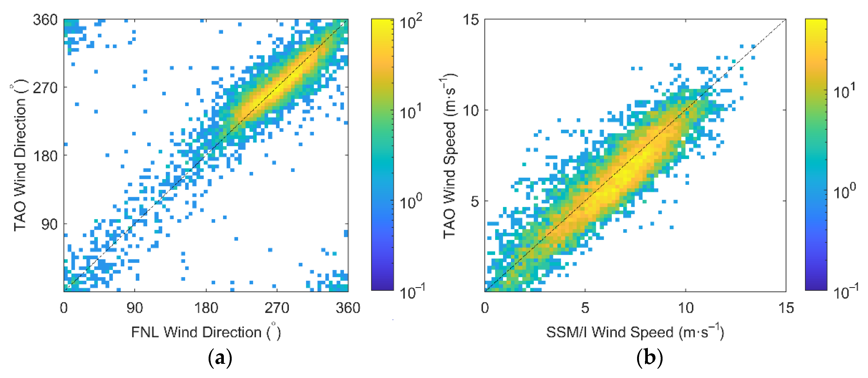
Figure 2.
Scatter plots of the NII, FNL, and SSM/I paired data. (a) Scatter plots of the FNL and NII wind speed. (b) Scatter plots of the FNL and SSM/I wind speed. The dashed line in this figure is the diagonal line.
Figure 2.
Scatter plots of the NII, FNL, and SSM/I paired data. (a) Scatter plots of the FNL and NII wind speed. (b) Scatter plots of the FNL and SSM/I wind speed. The dashed line in this figure is the diagonal line.

Figure 3.
Schematic diagram of BP neural network topology.
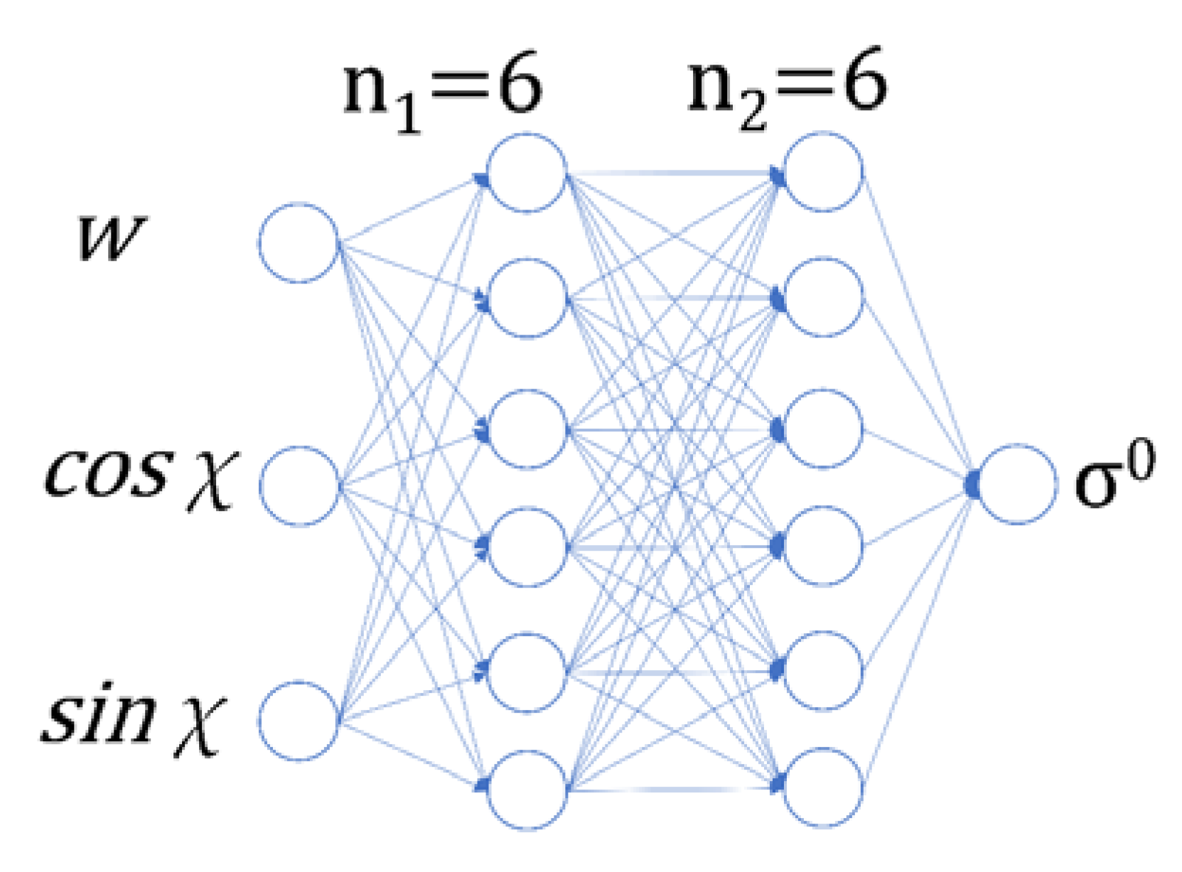
Figure 4.
Backscatter coefficient curves of HW-GMF and NSCAT-2 GMF. (a) Curves of HW-GMF for HH polarization. (b) Curves of NSCAT-2 GMF for HH polarization. (c) Curves of HW-GMF for VV polarization. (d) Curves of NSCAT-2 GMF for VV polarization.
Figure 4.
Backscatter coefficient curves of HW-GMF and NSCAT-2 GMF. (a) Curves of HW-GMF for HH polarization. (b) Curves of NSCAT-2 GMF for HH polarization. (c) Curves of HW-GMF for VV polarization. (d) Curves of NSCAT-2 GMF for VV polarization.
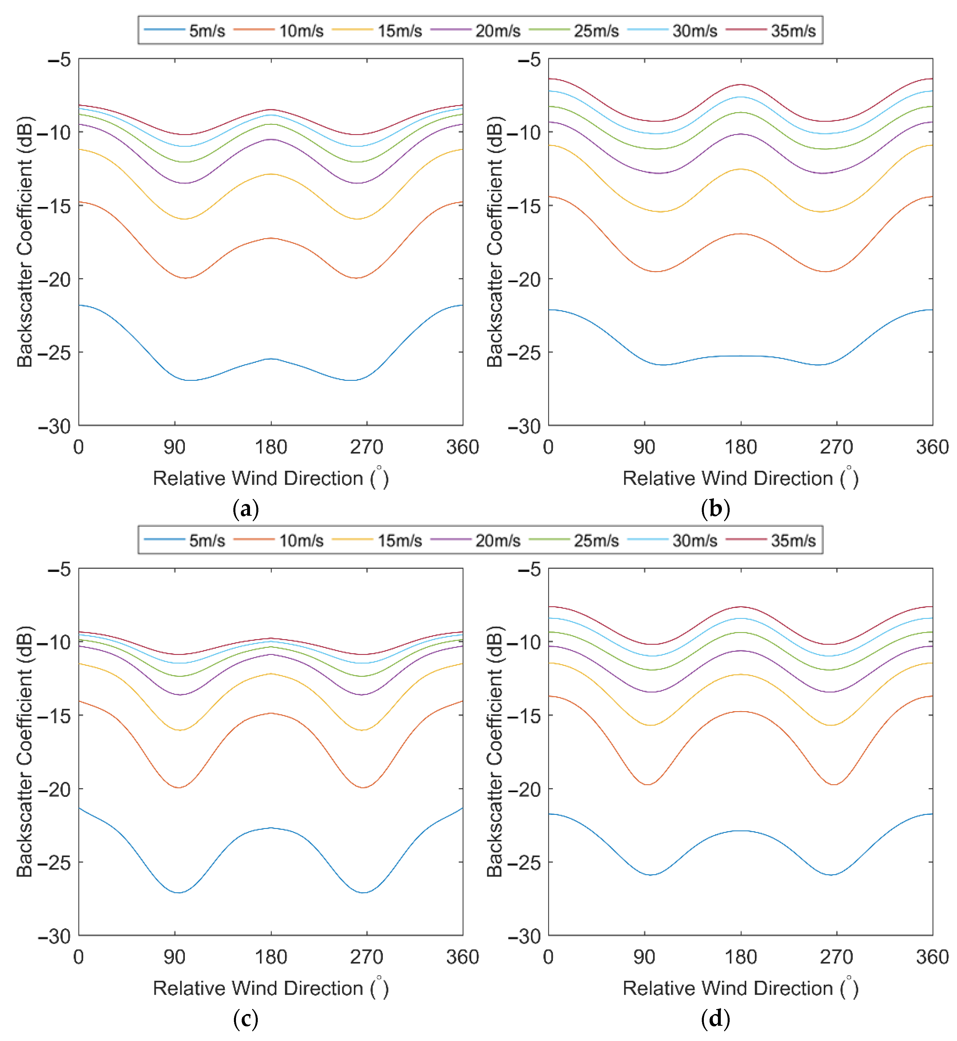
Figure 5.
Mean backscatter coefficient curves of HW-GMF and NSCAT-2 GMF; the red solid line corresponds to NSCAT-2 GMF, and the blue dashed line corresponds to HW-GMF. (a) HH polarization. (b) VV polarization.
Figure 5.
Mean backscatter coefficient curves of HW-GMF and NSCAT-2 GMF; the red solid line corresponds to NSCAT-2 GMF, and the blue dashed line corresponds to HW-GMF. (a) HH polarization. (b) VV polarization.

Figure 6.
Scatter plots of NSCAT-2 GMF σ0 and HY-2A σ0 paired data. (a) HH polarization. (b) VV polarization. The dashed line in this figure is the diagonal line.
Figure 6.
Scatter plots of NSCAT-2 GMF σ0 and HY-2A σ0 paired data. (a) HH polarization. (b) VV polarization. The dashed line in this figure is the diagonal line.
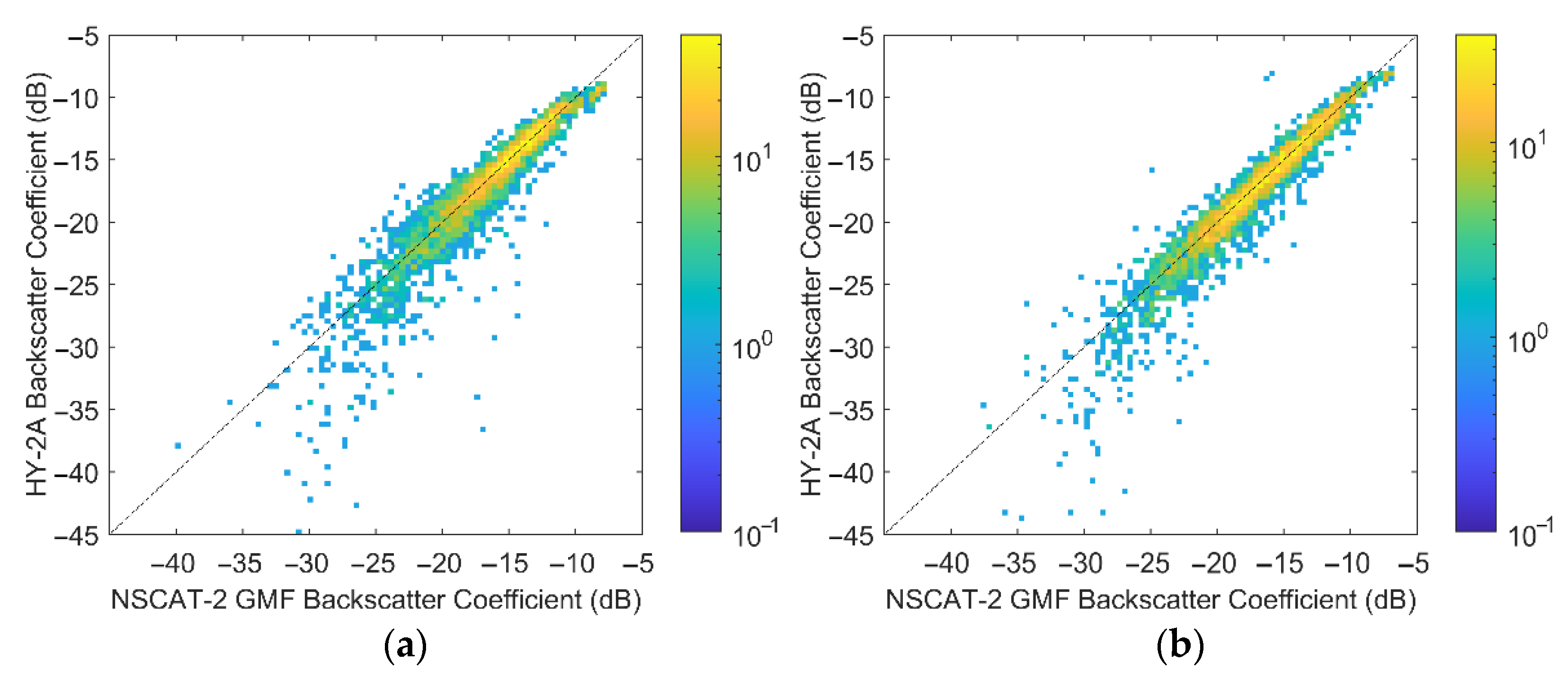
Figure 7.
Scatter plots of HW-GMF σ0 and HY-2A σ0 paired data. (a) HH polarization. (b) VV polarization. The dashed line in this figure is the diagonal line.
Figure 7.
Scatter plots of HW-GMF σ0 and HY-2A σ0 paired data. (a) HH polarization. (b) VV polarization. The dashed line in this figure is the diagonal line.

Figure 8.
Dependence of the σ0 residual on the SSM/I wind speed. The red circle in the figure is the mean value of deviation of the NSCAT-2 GMF model σ0 minus the HY-2A measurement σ0, and the blue asterisk is the mean value of deviation of the HW-GMF model σ0 minus the HY-2A measurement σ0. (a) HH polarization. (b) VV polarization. The dashed line in the figure represents a σ0 bias of 0.
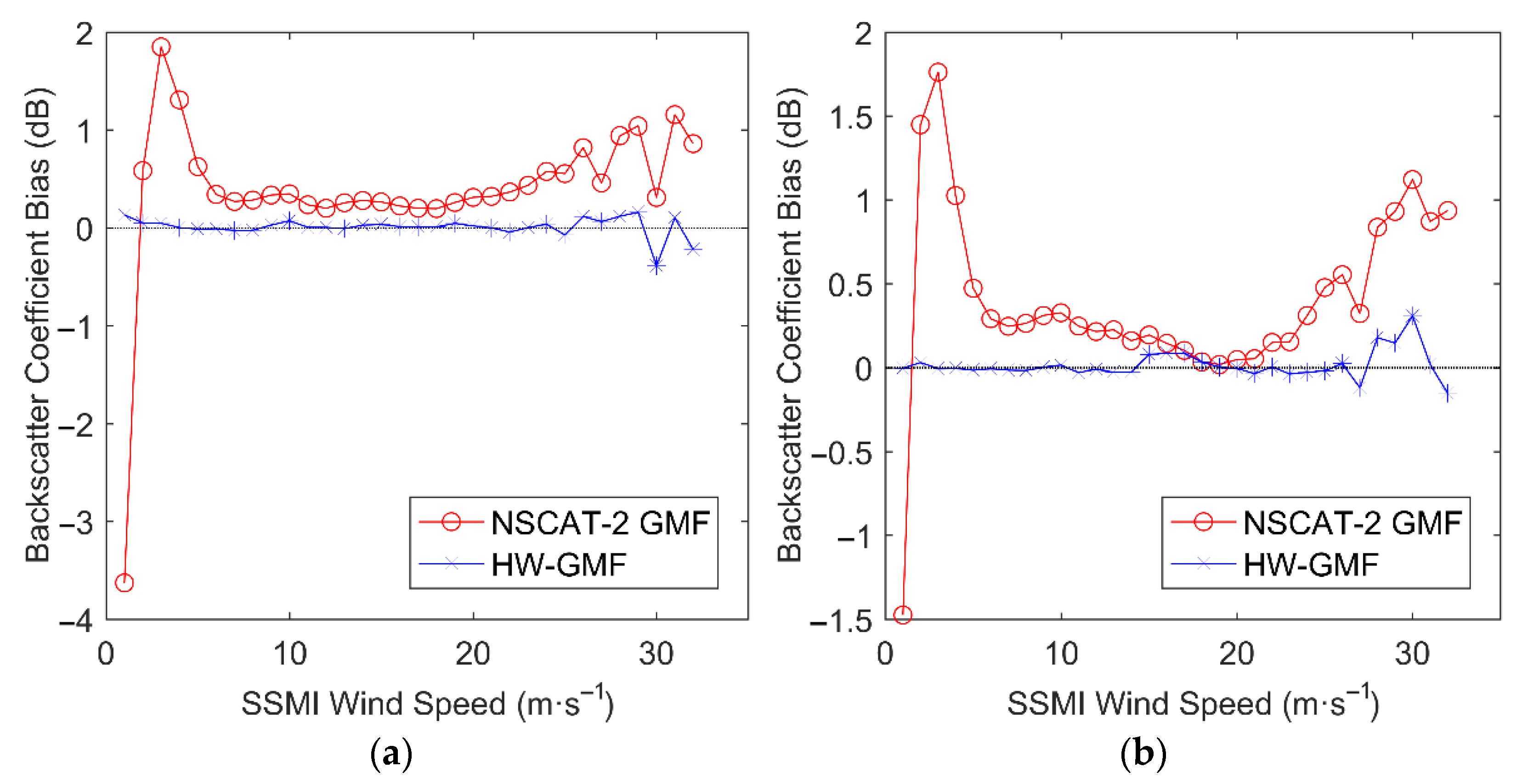
Figure 9.
Dependence of wind speed residual and percentage of the retrieved wind vectors on the SSM/I wind speed. (a) The result of error verification. The red circle in the figure is the mean value of deviation of the NSCAT-2 GMF retrieved wind speed minus the SSM/I wind speed, and the blue asterisk is the mean value of deviation of the HW-GMF retrieved wind speed minus the SSM/I wind speed. The dashed line in the figure represents a wind speed bias of 0. (b) The histogram of percentage of the retrieved wind vectors.
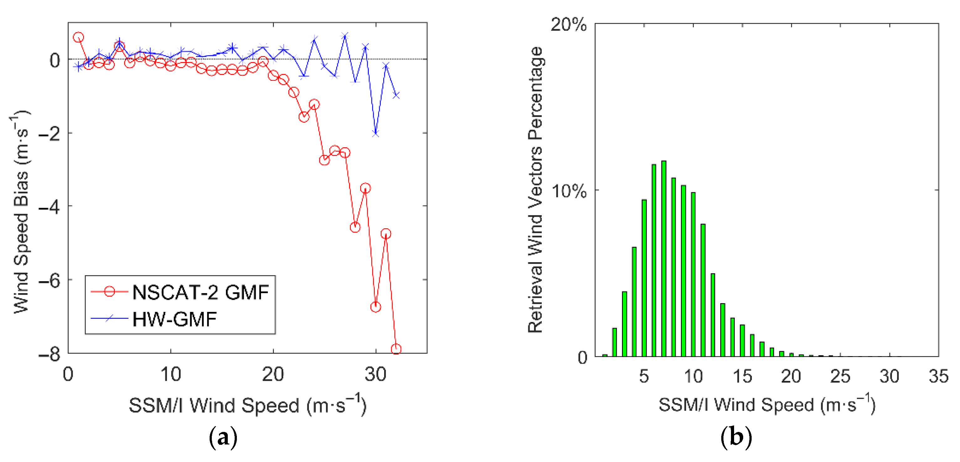
Figure 10.
RMSE of the HY-2A retrieved wind vectors against the SSM/I wind speed. The red circle in this figure is the RMSE of the NSCAT-2 GMF retrieved wind speed, and the blue asterisk is the RMSE of the HW-GMF retrieved wind speed.
Figure 10.
RMSE of the HY-2A retrieved wind vectors against the SSM/I wind speed. The red circle in this figure is the RMSE of the NSCAT-2 GMF retrieved wind speed, and the blue asterisk is the RMSE of the HW-GMF retrieved wind speed.

Figure 11.
The probability density functions (PDFs) of HY-2A and SSM/I wind speed. The black line in the figure is the PDF curve of SSMI wind speed, the red line in the figure is the PDF curve of NSCAT-2 GMF retrieved wind speed, and the blue line in the figure is the PDF curve of HW-GMF retrieved wind speed.

Figure 12.
Scatter plots of the wind direction retrieved by the NSCAT-2 and HW-GMF and the FNL wind direction. (a) Scatter plots of the NSCAT-2 GMF wind direction. (b) Scatter plots of the HW-GMF wind direction. The dashed line in this figure is the diagonal line.
Figure 12.
Scatter plots of the wind direction retrieved by the NSCAT-2 and HW-GMF and the FNL wind direction. (a) Scatter plots of the NSCAT-2 GMF wind direction. (b) Scatter plots of the HW-GMF wind direction. The dashed line in this figure is the diagonal line.
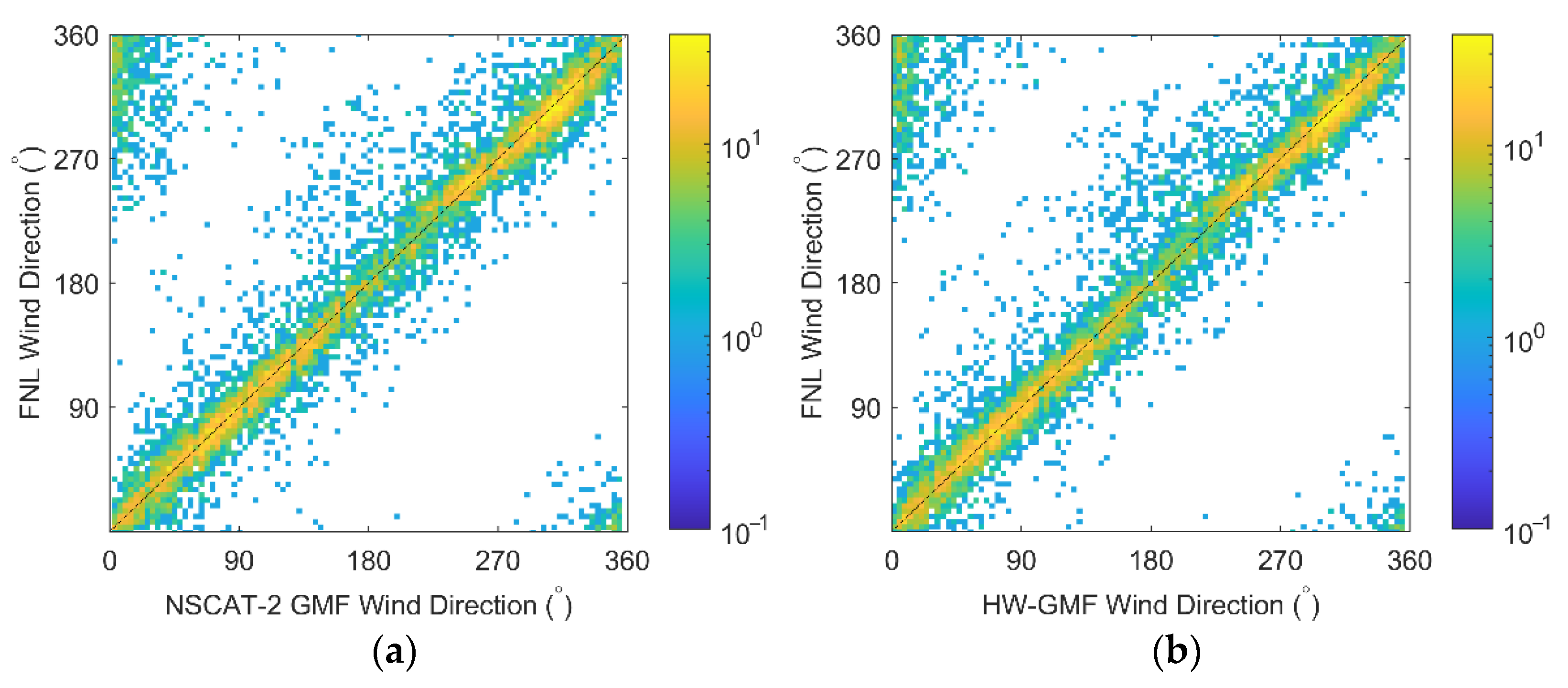

Table 1.
FNL and SSM/I wind field data and TAO sea surface wind velocity data statistical analysis.
| Bias | Standard Deviation | |
|---|---|---|
| FNL wind direction (°) | −0.3634 | 14.4150 |
| SSM/I wind speed (m/s) | −0.2579 | 0.9554 |
Table 2.
NII, SSM/I, and FNL sea surface wind velocity data statistical analysis.
| Bias | Standard Deviation | |
|---|---|---|
| SSM/I Wind Speed (m/s) | 0.5402 | 2.2347 |
| NII Wind Speed (m/s) | 0.6758 | 4.3049 |
Table 3.
The backscattering coefficients in HW-GMF of HH pol.
| 0° | 5° | 10° | 15° | 20° | 25° | 30° | 35° | 40° | 45° | 50° | 55° | 60° | 65° | 70° | 75° | 80° | 85° | 90° | 95° | 100° | 105° | 110° | 115° | 120° | 125° | 130° | 135° | 140° | 145° | 150° | 155° | 160° | 165° | 170° | 175° | 180° | |
|---|---|---|---|---|---|---|---|---|---|---|---|---|---|---|---|---|---|---|---|---|---|---|---|---|---|---|---|---|---|---|---|---|---|---|---|---|---|
| 1 m/s | −35.4675 | −35.5341 | −35.6079 | −35.6889 | −35.7765 | −35.8702 | −35.9695 | −36.0739 | −36.1831 | −36.2971 | −36.4161 | −36.5398 | −36.6668 | −36.7945 | −36.9186 | −37.0340 | −37.1357 | −37.2193 | −37.2822 | −37.3233 | −37.3433 | −37.3445 | −37.3305 | −37.3061 | −37.2763 | −37.2455 | −37.2167 | −37.1911 | −37.1683 | −37.1470 | −37.1259 | −37.1035 | −37.0788 | −37.0510 | −37.0195 | −36.9839 | −36.9440 |
| 2 m/s | −32.9884 | −33.0973 | −33.2198 | −33.3553 | −33.5031 | −33.6621 | −33.8312 | −34.0096 | −34.1965 | −34.3916 | −34.5945 | −34.8042 | −35.0181 | −35.2314 | −35.4377 | −35.6295 | −35.8003 | −35.9446 | −36.0596 | −36.1442 | −36.1992 | −36.2273 | −36.2328 | −36.2215 | −36.1999 | −36.1739 | −36.1479 | −36.1237 | −36.1012 | −36.0790 | −36.0549 | −36.0270 | −35.9940 | −35.9546 | −35.9081 | −35.8539 | −35.7914 |
| 3 m/s | −28.6308 | −28.7200 | −28.8434 | −29.0041 | −29.2026 | −29.4369 | −29.7019 | −29.9911 | −30.2976 | −30.6165 | −30.9465 | −31.2900 | −31.6501 | −32.0240 | −32.3974 | −32.7462 | −33.0460 | −33.2822 | −33.4540 | −33.5709 | −33.6477 | −33.7003 | −33.7426 | −33.7841 | −33.8280 | −33.8708 | −33.9024 | −33.9100 | −33.8843 | −33.8251 | −33.7432 | −33.6541 | −33.5701 | −33.4958 | −33.4315 | −33.3767 | −33.3327 |
| 4 m/s | −24.7055 | −24.7655 | −24.8610 | −24.9977 | −25.1782 | −25.4026 | −25.6675 | −25.9670 | −26.2937 | −26.6411 | −27.0048 | −27.3843 | −27.7810 | −28.1940 | −28.6134 | −29.0189 | −29.3845 | −29.6888 | −29.9221 | −30.0864 | −30.1923 | −30.2538 | −30.2845 | −30.2953 | −30.2921 | −30.2754 | −30.2411 | −30.1836 | −30.1012 | −29.9992 | −29.8878 | −29.7764 | −29.6683 | −29.5617 | −29.4540 | −29.3453 | −29.2392 |
| 5 m/s | −22.0130 | −22.0468 | −22.1144 | −22.2224 | −22.3749 | −22.5731 | −22.8149 | −23.0952 | −23.4066 | −23.7415 | −24.0935 | −24.4590 | −24.8369 | −25.2262 | −25.6209 | −26.0061 | −26.3596 | −26.6588 | −26.8880 | −27.0426 | −27.1270 | −27.1515 | −27.1286 | −27.0699 | −26.9845 | −26.8786 | −26.7559 | −26.6208 | −26.4799 | −26.3423 | −26.2156 | −26.1022 | −25.9980 | −25.8964 | −25.7929 | −25.6875 | −25.5840 |
| 6 m/s | −20.0895 | −20.1149 | −20.1732 | −20.2717 | −20.4153 | −20.6060 | −20.8425 | −21.1203 | −21.4325 | −21.7704 | −22.1258 | −22.4924 | −22.8662 | −23.2442 | −23.6215 | −23.9872 | −24.3238 | −24.6104 | −24.8296 | −24.9717 | −25.0358 | −25.0283 | −24.9593 | −24.8410 | −24.6853 | −24.5040 | −24.3088 | −24.1122 | −23.9271 | −23.7641 | −23.6277 | −23.5151 | −23.4176 | −23.3262 | −23.2348 | −23.1424 | −23.0517 |
| 7 m/s | −18.5452 | −18.5713 | −18.6304 | −18.7297 | −18.8748 | −19.0683 | −19.3098 | −19.5955 | −19.9187 | −20.2706 | −20.6417 | −21.0235 | −21.4091 | −21.7933 | −22.1704 | −22.5314 | −22.8623 | −23.1451 | −23.3626 | −23.5025 | −23.5601 | −23.5377 | −23.4435 | −23.2890 | −23.0887 | −22.8584 | −22.6157 | −22.3785 | −22.1632 | −21.9804 | −21.8326 | −21.7142 | −21.6152 | −21.5252 | −21.4376 | −21.3501 | −21.2639 |
| 8 m/s | −17.2028 | −17.2329 | −17.2957 | −17.3986 | −17.5475 | −17.7455 | −17.9929 | −18.2867 | −18.6206 | −18.9860 | −19.3727 | −19.7707 | −20.1710 | −20.5660 | −20.9486 | −21.3102 | −21.6389 | −21.9194 | −22.1360 | −22.2756 | −22.3311 | −22.3022 | −22.1949 | −22.0204 | −21.7942 | −21.5350 | −21.2638 | −21.0014 | −20.7653 | −20.5660 | −20.4052 | −20.2769 | −20.1710 | −20.0776 | −19.9895 | −19.9031 | −19.8179 |
| 9 m/s | −16.0019 | −16.0367 | −16.1037 | −16.2101 | −16.3619 | −16.5628 | −16.8135 | −17.1117 | −17.4517 | −17.8254 | −18.2224 | −18.6318 | −19.0429 | −19.4463 | −19.8333 | −20.1948 | −20.5201 | −20.7959 | −21.0081 | −21.1444 | −21.1966 | −21.1629 | −21.0479 | −20.8622 | −20.6218 | −20.3465 | −20.0589 | −19.7806 | −19.5294 | −19.3155 | −19.1410 | −19.0007 | −18.8858 | −18.7870 | −18.6971 | −18.6114 | −18.5274 |
| 10 m/s | −14.9258 | −14.9655 | −15.0363 | −15.1455 | −15.2989 | −15.5004 | −15.7513 | −16.0498 | −16.3912 | −16.7674 | −17.1686 | −17.5834 | −18.0000 | −18.4076 | −18.7961 | −19.1556 | −19.4756 | −19.7444 | −19.9493 | −20.0792 | −20.1262 | −20.0878 | −19.9677 | −19.7759 | −19.5283 | −19.2449 | −18.9482 | −18.6595 | −18.3963 | −18.1689 | −17.9802 | −17.8268 | −17.7017 | −17.5965 | −17.5041 | −17.4188 | −17.3366 |
| 11 m/s | −13.9692 | −14.0135 | −14.0877 | −14.1988 | −14.3526 | −14.5530 | −14.8016 | −15.0972 | −15.4357 | −15.8099 | −16.2102 | −16.6250 | −17.0423 | −17.4502 | −17.8373 | −18.1930 | −18.5067 | −18.7674 | −18.9640 | −19.0863 | −19.1271 | −19.0842 | −18.9607 | −18.7662 | −18.5159 | −18.2292 | −17.9276 | −17.6319 | −17.3586 | −17.1186 | −16.9160 | −16.7493 | −16.6131 | −16.5005 | −16.4045 | −16.3188 | −16.2382 |
| 12 m/s | −13.1268 | −13.1753 | −13.2524 | −13.3647 | −13.5178 | −13.7156 | −13.9601 | −14.2504 | −14.5832 | −14.9518 | −15.3471 | −15.7579 | −16.1721 | −16.5769 | −16.9603 | −17.3110 | −17.6180 | −17.8707 | −18.0589 | −18.1738 | −18.2089 | −18.1621 | −18.0368 | −17.8419 | −17.5917 | −17.3046 | −17.0010 | −16.7004 | −16.4189 | −16.1676 | −15.9519 | −15.7721 | −15.6247 | −15.5040 | −15.4034 | −15.3161 | −15.2360 |
| 13 m/s | −12.3909 | −12.4430 | −12.5224 | −12.6353 | −12.7869 | −12.9811 | −13.2201 | −13.5035 | −13.8283 | −14.1888 | −14.5763 | −14.9801 | −15.3880 | −15.7872 | −16.1651 | −16.5097 | −16.8099 | −17.0551 | −17.2359 | −17.3442 | −17.3744 | −17.3251 | −17.1993 | −17.0056 | −16.7574 | −16.4719 | −16.1681 | −15.8644 | −15.5765 | −15.3156 | −15.0884 | −14.8967 | −14.7385 | −14.6093 | −14.5031 | −14.4131 | −14.3326 |
| 14 m/s | −11.7517 | −11.8069 | −11.8880 | −12.0008 | −12.1502 | −12.3402 | −12.5728 | −12.8480 | −13.1635 | −13.5140 | −13.8916 | −14.2861 | −14.6855 | −15.0771 | −15.4479 | −15.7857 | −16.0789 | −16.3173 | −16.4916 | −16.5944 | −16.6211 | −16.5702 | −16.4451 | −16.2539 | −16.0090 | −15.7265 | −15.4240 | −15.1189 | −14.8264 | −14.5581 | −14.3213 | −14.1192 | −13.9513 | −13.8139 | −13.7018 | −13.6083 | −13.5262 |
| 15 m/s | −11.1989 | −11.2566 | −11.3388 | −11.4509 | −11.5976 | −11.7826 | −12.0081 | −12.2745 | −12.5797 | −12.9191 | −13.2853 | −13.6688 | −14.0580 | −14.4403 | −14.8028 | −15.1330 | −15.4193 | −15.6511 | −15.8198 | −15.9183 | −15.9423 | −15.8910 | −15.7677 | −15.5798 | −15.3392 | −15.0607 | −14.7608 | −14.4560 | −14.1610 | −13.8874 | −13.6433 | −13.4328 | −13.2565 | −13.1118 | −12.9938 | −12.8963 | −12.8121 |
| 16 m/s | −10.7220 | −10.7815 | −10.8642 | −10.9750 | −11.1185 | −11.2982 | −11.5163 | −11.7733 | −12.0676 | −12.3950 | −12.7490 | −13.1203 | −13.4981 | −13.8700 | −14.2231 | −14.5450 | −14.8240 | −15.0497 | −15.2133 | −15.3082 | −15.3306 | −15.2797 | −15.1587 | −14.9750 | −14.7394 | −14.4658 | −14.1698 | −13.8668 | −13.5712 | −13.2947 | −13.0456 | −12.8288 | −12.6458 | −12.4947 | −12.3714 | −12.2698 | −12.1832 |
| 17 m/s | −10.3111 | −10.3717 | −10.4543 | −10.5635 | −10.7034 | −10.8774 | −11.0878 | −11.3352 | −11.6183 | −11.9334 | −12.2744 | −12.6328 | −12.9982 | −13.3587 | −13.7017 | −14.0148 | −14.2862 | −14.5057 | −14.6646 | −14.7566 | −14.7779 | −14.7280 | −14.6101 | −14.4310 | −14.2010 | −13.9332 | −13.6421 | −13.3425 | −13.0482 | −12.7708 | −12.5189 | −12.2980 | −12.1100 | −11.9539 | −11.8259 | −11.7207 | −11.6315 |
| 18 m/s | −9.9570 | −10.0183 | −10.1004 | −10.2075 | −10.3435 | −10.5117 | −10.7142 | −10.9519 | −11.2236 | −11.5261 | −11.8538 | −12.1989 | −12.5514 | −12.8998 | −13.2320 | −13.5357 | −13.7993 | −14.0126 | −14.1670 | −14.2563 | −14.2770 | −14.2286 | −14.1142 | −13.9402 | −13.7163 | −13.4549 | −13.1696 | −12.8747 | −12.5834 | −12.3071 | −12.0546 | −11.8315 | −11.6403 | −11.4804 | −11.3487 | −11.2403 | −11.1489 |
| 19 m/s | −9.6518 | −9.7133 | −9.7944 | −9.8991 | −10.0310 | −10.1932 | −10.3879 | −10.6158 | −10.8762 | −11.1661 | −11.4804 | −11.8119 | −12.1510 | −12.4870 | −12.8080 | −13.1019 | −13.3574 | −13.5643 | −13.7142 | −13.8011 | −13.8215 | −13.7748 | −13.6641 | −13.4955 | −13.2782 | −13.0238 | −12.7453 | −12.4563 | −12.1694 | −11.8959 | −11.6445 | −11.4210 | −11.2282 | −11.0659 | −10.9316 | −10.8207 | −10.7274 |
| 20 m/s | −9.3885 | −9.4497 | −9.5295 | −9.6315 | −9.7592 | −9.9154 | −10.1022 | −10.3205 | −10.5696 | −10.8470 | −11.1481 | −11.4658 | −11.7916 | −12.1148 | −12.4241 | −12.7080 | −12.9551 | −13.1555 | −13.3010 | −13.3855 | −13.4056 | −13.3609 | −13.2542 | −13.0912 | −12.8808 | −12.6339 | −12.3629 | −12.0806 | −11.7995 | −11.5303 | −11.2816 | −11.0592 | −10.8662 | −10.7028 | −10.5669 | −10.4542 | −10.3595 |
| 21 m/s | −9.1609 | −9.2216 | −9.2998 | −9.3989 | −9.5222 | −9.6724 | −9.8515 | −10.0603 | −10.2984 | −10.5636 | −10.8514 | −11.1556 | −11.4678 | −11.7782 | −12.0758 | −12.3493 | −12.5879 | −12.7817 | −12.9226 | −13.0047 | −13.0247 | −12.9820 | −12.8794 | −12.7222 | −12.5189 | −12.2799 | −12.0169 | −11.7423 | −11.4679 | −11.2042 | −10.9595 | −10.7396 | −10.5477 | −10.3844 | −10.2477 | −10.1340 | −10.0385 |
| 22 m/s | −8.9640 | −9.0237 | −9.1001 | −9.1962 | −9.3151 | −9.4593 | −9.6308 | −9.8304 | −10.0578 | −10.3109 | −10.5858 | −10.8766 | −11.1755 | −11.4730 | −11.7588 | −12.0219 | −12.2517 | −12.4388 | −12.5751 | −12.6548 | −12.6746 | −12.6340 | −12.5354 | −12.3842 | −12.1882 | −11.9573 | −11.7028 | −11.4365 | −11.1697 | −10.9124 | −10.6727 | −10.4565 | −10.2668 | −10.1045 | −9.9680 | −9.8541 | −9.7582 |
| 23 m/s | −8.7931 | −8.8518 | −8.9261 | −9.0191 | −9.1336 | −9.2719 | −9.4359 | −9.6266 | −9.8436 | −10.0850 | −10.3473 | −10.6250 | −10.9107 | −11.1955 | −11.4695 | −11.7221 | −11.9432 | −12.1234 | −12.2550 | −12.3322 | −12.3519 | −12.3133 | −12.2189 | −12.0736 | −11.8849 | −11.6624 | −11.4168 | −11.1592 | −10.9006 | −10.6505 | −10.4167 | −10.2050 | −10.0185 | −9.8580 | −9.7225 | −9.6089 | −9.5133 |
| 24 m/s | −8.6446 | −8.7020 | −8.7742 | −8.8640 | −8.9741 | −9.1066 | −9.2634 | −9.4454 | −9.6523 | −9.8824 | −10.1325 | −10.3974 | −10.6702 | −10.9424 | −11.2047 | −11.4469 | −11.6592 | −11.8326 | −11.9594 | −12.0342 | −12.0535 | −12.0170 | −11.9266 | −11.7872 | −11.6060 | −11.3920 | −11.1554 | −10.9069 | −10.6569 | −10.4145 | −10.1874 | −9.9809 | −9.7982 | −9.6405 | −9.5065 | −9.3939 | −9.2990 |
| 25 m/s | −8.5153 | −8.5712 | −8.6412 | −8.7278 | −8.8335 | −8.9604 | −9.1102 | −9.2837 | −9.4809 | −9.7001 | −9.9384 | −10.1908 | −10.4510 | −10.7111 | −10.9618 | −11.1937 | −11.3973 | −11.5638 | −11.6859 | −11.7580 | −11.7770 | −11.7424 | −11.6561 | −11.5226 | −11.3488 | −11.1433 | −10.9159 | −10.6766 | −10.4355 | −10.2013 | −9.9813 | −9.7806 | −9.6024 | −9.4479 | −9.3162 | −9.2050 | −9.1112 |
| 26 m/s | −8.4024 | −8.4567 | −8.5244 | −8.6078 | −8.7092 | −8.8306 | −8.9736 | −9.1391 | −9.3268 | −9.5356 | −9.7624 | −10.0028 | −10.2509 | −10.4989 | −10.7384 | −10.9602 | −11.1551 | −11.3148 | −11.4320 | −11.5016 | −11.5203 | −11.4875 | −11.4051 | −11.2774 | −11.1110 | −10.9139 | −10.6957 | −10.4658 | −10.2338 | −10.0081 | −9.7954 | −9.6009 | −9.4277 | −9.2769 | −9.1479 | −9.0387 | −8.9463 |
| 27 m/s | −8.3036 | −8.3563 | −8.4216 | −8.5018 | −8.5990 | −8.7151 | −8.8515 | −9.0092 | −9.1879 | −9.3866 | −9.6024 | −9.8313 | −10.0675 | −10.3039 | −10.5325 | −10.7443 | −10.9307 | −11.0836 | −11.1961 | −11.2630 | −11.2813 | −11.2503 | −11.1717 | −11.0497 | −10.8905 | −10.7019 | −10.4928 | −10.2723 | −10.0495 | −9.8323 | −9.6273 | −9.4394 | −9.2714 | −9.1247 | −8.9988 | −8.8918 | −8.8012 |
| 28 m/s | −8.2169 | −8.2679 | −8.3309 | −8.4079 | −8.5010 | −8.6119 | −8.7420 | −8.8922 | −9.0623 | −9.2512 | −9.4565 | −9.6743 | −9.8991 | −10.1243 | −10.3422 | −10.5443 | −10.7224 | −10.8687 | −10.9764 | −11.0407 | −11.0585 | −11.0292 | −10.9543 | −10.8379 | −10.6858 | −10.5055 | −10.3054 | −10.0942 | −9.8806 | −9.6720 | −9.4748 | −9.2935 | −9.1312 | −8.9889 | −8.8663 | −8.7619 | −8.6733 |
| 29 m/s | −8.1407 | −8.1900 | −8.2506 | −8.3245 | −8.4136 | −8.5195 | −8.6435 | −8.7865 | −8.9483 | −9.1280 | −9.3232 | −9.5302 | −9.7441 | −9.9585 | −10.1660 | −10.3587 | −10.5287 | −10.6684 | −10.7715 | −10.8332 | −10.8505 | −10.8227 | −10.7515 | −10.6405 | −10.4953 | −10.3231 | −10.1319 | −9.9299 | −9.7254 | −9.5254 | −9.3360 | −9.1616 | −9.0049 | −8.8672 | −8.7482 | −8.6467 | −8.5603 |
| 30 m/s | −8.0736 | −8.1211 | −8.1794 | −8.2502 | −8.3354 | −8.4365 | −8.5547 | −8.6907 | −8.8447 | −9.0154 | −9.2009 | −9.3977 | −9.6011 | −9.8050 | −10.0025 | −10.1861 | −10.3482 | −10.4816 | −10.5802 | −10.6392 | −10.6560 | −10.6297 | −10.5620 | −10.4562 | −10.3178 | −10.1535 | −9.9709 | −9.7780 | −9.5824 | −9.3909 | −9.2093 | −9.0417 | −8.8908 | −8.7579 | −8.6427 | −8.5442 | −8.4602 |
| 31 m/s | −8.0142 | −8.0600 | −8.1160 | −8.1838 | −8.2652 | −8.3617 | −8.4743 | −8.6037 | −8.7501 | −8.9124 | −9.0886 | −9.2756 | −9.4689 | −9.6627 | −9.8506 | −10.0254 | −10.1798 | −10.3071 | −10.4011 | −10.4576 | −10.4738 | −10.4490 | −10.3846 | −10.2839 | −10.1521 | −9.9954 | −9.8213 | −9.6372 | −9.4504 | −9.2673 | −9.0934 | −8.9326 | −8.7876 | −8.6594 | −8.5482 | −8.4527 | −8.3713 |
| 32 m/s | −7.9617 | −8.0057 | −8.0594 | −8.1244 | −8.2021 | −8.2941 | −8.4013 | −8.5244 | −8.6635 | −8.8177 | −8.9851 | −9.1628 | −9.3463 | −9.5306 | −9.7092 | −9.8755 | −10.0226 | −10.1438 | −10.2335 | −10.2875 | −10.3031 | −10.2797 | −10.2185 | −10.1227 | −9.9971 | −9.8480 | −9.6820 | −9.5065 | −9.3282 | −9.1534 | −8.9870 | −8.8330 | −8.6938 | −8.5705 | −8.4632 | −8.3710 | −8.2922 |
| 33 m/s | −7.9151 | −7.9574 | −8.0089 | −8.0710 | −8.1452 | −8.2328 | −8.3349 | −8.4520 | −8.5842 | −8.7307 | −8.8896 | −9.0583 | −9.2326 | −9.4076 | −9.5774 | −9.7356 | −9.8755 | −9.9909 | −10.0764 | −10.1280 | −10.1430 | −10.1208 | −10.0627 | −9.9716 | −9.8522 | −9.7102 | −9.5522 | −9.3849 | −9.2150 | −9.0481 | −8.8892 | −8.7418 | −8.6083 | −8.4899 | −8.3866 | −8.2976 | −8.2215 |
| 34 m/s | −7.8736 | −7.9142 | −7.9635 | −8.0229 | −8.0937 | −8.1772 | −8.2743 | −8.3856 | −8.5112 | −8.6503 | −8.8013 | −8.9614 | −9.1269 | −9.2931 | −9.4544 | −9.6047 | −9.7377 | −9.8475 | −9.9290 | −9.9782 | −9.9926 | −9.9716 | −9.9165 | −9.8299 | −9.7163 | −9.5813 | −9.4309 | −9.2717 | −9.1098 | −8.9507 | −8.7989 | −8.6581 | −8.5303 | −8.4167 | −8.3174 | −8.2317 | −8.1583 |
| 35 m/s | −7.8367 | −7.8756 | −7.9227 | −7.9794 | −8.0469 | −8.1265 | −8.2189 | −8.3247 | −8.4440 | −8.5761 | −8.7194 | −8.8713 | −9.0284 | −9.1862 | −9.3394 | −9.4822 | −9.6086 | −9.7130 | −9.7906 | −9.8374 | −9.8513 | −9.8315 | −9.7791 | −9.6969 | −9.5889 | −9.4605 | −9.3176 | −9.1661 | −9.0119 | −8.8603 | −8.7156 | −8.5810 | −8.4588 | −8.3499 | −8.2546 | −8.1723 | −8.1016 |
Table 4.
The backscattering coefficients in HW-GMF of VV pol.
| 0° | 5° | 10° | 15° | 20° | 25° | 30° | 35° | 40° | 45° | 50° | 55° | 60° | 65° | 70° | 75° | 80° | 85° | 90° | 95° | 100° | 105° | 110° | 115° | 120° | 125° | 130° | 135° | 140° | 145° | 150° | 155° | 160° | 165° | 170° | 175° | 180° | |
|---|---|---|---|---|---|---|---|---|---|---|---|---|---|---|---|---|---|---|---|---|---|---|---|---|---|---|---|---|---|---|---|---|---|---|---|---|---|
| 1 m/s | −35.9378 | −36.0155 | −36.0955 | −36.1738 | −36.2475 | −36.3145 | −36.3749 | −36.4304 | −36.4845 | −36.5423 | −36.6099 | −36.6934 | −36.7976 | −36.923 | −37.0639 | −37.2087 | −37.3425 | −37.4509 | −37.5235 | −37.5545 | −37.5433 | −37.4942 | −37.4159 | −37.3215 | −37.2256 | −37.1408 | −37.0742 | −37.0266 | −36.9933 | −36.9675 | −36.9423 | −36.9119 | −36.8724 | −36.8221 | −36.7611 | −36.6914 | −36.6158 |
| 2 m/s | −33.2531 | −33.3233 | −33.408 | −33.5035 | −33.6048 | −33.7075 | −33.8083 | −33.9065 | −34.0039 | −34.1052 | −34.2171 | −34.347 | −34.5005 | −34.6782 | −34.8728 | −35.0692 | −35.2488 | −35.3939 | −35.4917 | −35.5356 | −35.5248 | −35.4645 | −35.3655 | −35.2436 | −35.117 | −35.0016 | −34.9067 | −34.8332 | −34.7755 | −34.7252 | −34.6743 | −34.6172 | −34.5513 | −34.477 | −34.3972 | −34.316 | −34.2376 |
| 3 m/s | −29.0027 | −29.2501 | −29.4524 | −29.6204 | −29.768 | −29.9106 | −30.0632 | −30.2386 | −30.4454 | −30.6872 | −30.9624 | −31.2643 | −31.5821 | −31.9025 | −32.2106 | −32.4916 | −32.7322 | −32.9208 | −33.0489 | −33.1109 | −33.105 | −33.033 | −32.9003 | −32.7164 | −32.4937 | −32.247 | −31.9924 | −31.7453 | −31.5196 | −31.3255 | −31.1692 | −31.0521 | −30.9709 | −30.9183 | −30.8835 | −30.8535 | −30.8143 |
| 4 m/s | −24.7618 | −25.014 | −25.2307 | −25.4233 | −25.6064 | −25.7967 | −26.01 | −26.2597 | −26.5543 | −26.8965 | −27.2826 | −27.7025 | −28.1406 | −28.5778 | −28.9929 | −29.365 | −29.6749 | −29.9068 | −30.049 | −30.0951 | −30.044 | −29.8999 | −29.6729 | −29.3777 | −29.0332 | −28.661 | −28.2832 | −27.9208 | −27.5913 | −27.3075 | −27.0765 | −26.8994 | −26.7717 | −26.684 | −26.6234 | −26.5746 | −26.5214 |
| 5 m/s | −21.51 | −21.737 | −21.9375 | −22.1225 | −22.3068 | −22.5067 | −22.7383 | −23.0149 | −23.3453 | −23.7323 | −24.1712 | −24.6507 | −25.1528 | −25.6546 | −26.1304 | −26.554 | −26.9015 | −27.1528 | −27.2933 | −27.3154 | −27.2184 | −27.0092 | −26.7016 | −26.3157 | −25.8761 | −25.4098 | −24.944 | −24.503 | −24.1065 | −23.768 | −23.4943 | −23.2857 | −23.1363 | −23.0356 | −22.9693 | −22.9213 | −22.8747 |
| 6 m/s | −19.1936 | −19.3943 | −19.5759 | −19.7489 | −19.9273 | −20.127 | −20.3633 | −20.6496 | −20.9946 | −21.4013 | −21.8655 | −22.3754 | −22.9122 | −23.451 | −23.9633 | −24.4194 | −24.7916 | −25.0564 | −25.1968 | −25.204 | −25.0777 | −24.8267 | −24.4681 | −24.0258 | −23.5287 | −23.0075 | −22.4922 | −22.0088 | −21.5776 | −21.2118 | −20.9173 | −20.6934 | −20.5333 | −20.4258 | −20.3565 | −20.3093 | −20.2677 |
| 7 m/s | −17.4844 | −17.6631 | −17.8286 | −17.9908 | −18.1628 | −18.3596 | −18.596 | −18.8847 | −19.2346 | −19.6492 | −20.1248 | −20.6501 | −21.2063 | −21.7679 | −22.3048 | −22.785 | −23.178 | −23.4578 | −23.6054 | −23.6107 | −23.4736 | −23.2041 | −22.8212 | −22.3517 | −21.8269 | −21.28 | −20.7422 | −20.2401 | −19.7938 | −19.4158 | −19.1111 | −18.8782 | −18.7099 | −18.595 | −18.5194 | −18.4674 | −18.4235 |
| 8 m/s | −16.1536 | −16.3133 | −16.4644 | −16.6162 | −16.7807 | −16.972 | −17.2039 | −17.4889 | −17.8358 | −18.2483 | −18.7238 | −19.2518 | −19.8142 | −20.3857 | −20.9357 | −21.4311 | −21.8395 | −22.1331 | −22.2912 | −22.3026 | −22.1671 | −21.895 | −21.5066 | −21.0303 | −20.4987 | −19.946 | −19.404 | −18.8989 | −18.4504 | −18.07 | −17.7622 | −17.5249 | −17.3508 | −17.2289 | −17.1456 | −17.0864 | −17.0367 |
| 9 m/s | −15.0787 | −15.2216 | −15.3594 | −15.5006 | −15.6564 | −15.8396 | −16.0633 | −16.3392 | −16.6763 | −17.0786 | −17.544 | −18.0635 | −18.6199 | −19.1889 | −19.7402 | −20.2405 | −20.6567 | −20.9597 | −21.1275 | −21.1482 | −21.0209 | −20.7562 | −20.3749 | −19.9057 | −19.3819 | −18.8375 | −18.3041 | −17.8075 | −17.3661 | −16.991 | −16.6858 | −16.4483 | −16.2713 | −16.1442 | −16.0543 | −15.9882 | −15.9324 |
| 10 m/s | −14.1934 | −14.3214 | −14.4469 | −14.5777 | −14.7239 | −14.8974 | −15.1104 | −15.3738 | −15.6964 | −16.0823 | −16.5305 | −17.0327 | −17.5733 | −18.1293 | −18.6716 | −19.1671 | −19.583 | −19.8895 | −20.0642 | −20.0943 | −19.9786 | −19.7272 | −19.361 | −18.9083 | −18.4022 | −17.8761 | −17.3605 | −16.8802 | −16.4529 | −16.0885 | −15.7906 | −15.5565 | −15.3794 | −15.2495 | −15.1549 | −15.0832 | −15.0223 |
| 11 m/s | −13.4568 | −13.5716 | −13.6861 | −13.807 | −13.9437 | −14.107 | −14.308 | −14.5572 | −14.8626 | −15.2287 | −15.655 | −16.1342 | −16.6523 | −17.1876 | −17.7126 | −18.1954 | −18.6038 | −18.9082 | −19.0861 | −19.1244 | −19.0213 | −18.7865 | −18.4402 | −18.01 | −17.528 | −17.0266 | −16.5348 | −16.0762 | −15.6674 | −15.3178 | −15.0302 | −14.8022 | −14.6275 | −14.4967 | −14.3992 | −14.3236 | −14.259 |
| 12 m/s | −12.8401 | −12.9437 | −13.0484 | −13.1604 | −13.2881 | −13.4414 | −13.6304 | −13.8647 | −14.1521 | −14.497 | −14.899 | −15.3522 | −15.8436 | −16.3533 | −16.8554 | −17.3197 | −17.715 | −18.0126 | −18.1903 | −18.2348 | −18.144 | −17.927 | −17.6031 | −17.1988 | −16.7447 | −16.2716 | −15.8072 | −15.3734 | −14.9858 | −14.6531 | −14.3779 | −14.1579 | −13.9871 | −13.8572 | −13.7583 | −13.6803 | −13.6133 |
| 13 m/s | −12.3216 | −12.4156 | −12.5118 | −12.616 | −12.7355 | −12.8794 | −13.0569 | −13.2769 | −13.5466 | −13.8701 | −14.2475 | −14.6735 | −15.1364 | −15.6178 | −16.0937 | −16.5356 | −16.9139 | −17.2011 | −17.3755 | −17.4242 | −17.3447 | −17.1456 | −16.8449 | −16.4678 | −16.0433 | −15.6003 | −15.1646 | −14.757 | −14.3918 | −14.0771 | −13.8154 | −13.6044 | −13.4388 | −13.311 | −13.2119 | −13.1326 | −13.0642 |
| 14 m/s | −11.8839 | −11.9697 | −12.0587 | −12.156 | −12.2684 | −12.4038 | −12.5708 | −12.7774 | −13.0302 | −13.3333 | −13.6867 | −14.0858 | −14.5199 | −14.9722 | −15.4203 | −15.8378 | −16.1966 | −16.4708 | −16.6397 | −16.6906 | −16.6211 | −16.439 | −16.1612 | −15.8113 | −15.4165 | −15.0037 | −14.597 | −14.2158 | −13.8732 | −13.5767 | −13.3287 | −13.1273 | −12.9676 | −12.8426 | −12.7443 | −12.6646 | −12.5956 |
| 15 m/s | −11.5127 | −11.5916 | −11.6745 | −11.766 | −11.8722 | −12.0002 | −12.1577 | −12.3521 | −12.5895 | −12.8734 | −13.2042 | −13.5774 | −13.9836 | −14.407 | −14.8272 | −15.2194 | −15.5575 | −15.8172 | −15.9787 | −16.0303 | −15.9693 | −15.803 | −15.547 | −15.2234 | −14.8574 | −14.4739 | −14.0955 | −13.7399 | −13.4194 | −13.1408 | −12.9065 | −12.7148 | −12.5613 | −12.4397 | −12.3429 | −12.2635 | −12.1946 |
| 16 m/s | −11.1966 | −11.2698 | −11.3475 | −11.4341 | −11.5349 | −11.6564 | −11.8056 | −11.9891 | −12.2123 | −12.4787 | −12.7885 | −13.1376 | −13.5172 | −13.9129 | −14.3057 | −14.6728 | −14.9899 | −15.2342 | −15.3874 | −15.4383 | −15.3844 | −15.2323 | −14.9967 | −14.6978 | −14.3591 | −14.0037 | −13.6521 | −13.321 | −13.0215 | −12.7602 | −12.5391 | −12.357 | −12.2097 | −12.0919 | −11.997 | −11.9185 | −11.8502 |
| 17 m/s | −10.9263 | −10.9945 | −11.068 | −11.1504 | −11.2466 | −11.3625 | −11.5043 | −11.6781 | −11.8887 | −12.1392 | −12.4297 | −12.7564 | −13.1112 | −13.4808 | −13.8474 | −14.1902 | −14.4865 | −14.7152 | −14.8594 | −14.9086 | −14.8605 | −14.7213 | −14.5043 | −14.2284 | −13.9151 | −13.5858 | −13.2596 | −12.9514 | −12.6718 | −12.4268 | −12.2184 | −12.0455 | −11.9046 | −11.7906 | −11.698 | −11.6208 | −11.5536 |
| 18 m/s | −10.6941 | −10.7581 | −10.8278 | −10.9067 | −10.999 | −11.11 | −11.2454 | −11.4105 | −11.6099 | −11.846 | −12.119 | −12.4253 | −12.7571 | −13.1022 | −13.4443 | −13.7638 | −14.04 | −14.2534 | −14.3884 | −14.4352 | −14.3918 | −14.2638 | −14.0637 | −13.8089 | −13.5192 | −13.2142 | −12.9113 | −12.6245 | −12.3634 | −12.1338 | −11.9374 | −11.7734 | −11.6387 | −11.5288 | −11.4387 | −11.3631 | −11.2971 |
| 19 m/s | −10.4936 | −10.554 | −10.6206 | −10.6964 | −10.7853 | −10.8921 | −11.0219 | −11.1794 | −11.3686 | −11.5919 | −11.849 | −12.1365 | −12.4472 | −12.7697 | −13.0888 | −13.3865 | −13.6436 | −13.8422 | −13.9678 | −14.0117 | −13.9721 | −13.8541 | −13.6693 | −13.4337 | −13.1655 | −12.8828 | −12.6016 | −12.3346 | −12.0908 | −11.8754 | −11.6903 | −11.5348 | −11.4061 | −11.3003 | −11.2129 | −11.1391 | −11.0747 |
| 20 m/s | −10.3199 | −10.3771 | −10.4409 | −10.514 | −10.6 | −10.7031 | −10.8279 | −10.9786 | −11.1588 | −11.3704 | −11.6131 | −11.8836 | −12.175 | −12.4766 | −12.7744 | −13.0517 | −13.2908 | −13.4752 | −13.5918 | −13.6325 | −13.5958 | −13.4866 | −13.3156 | −13.0975 | −12.849 | −12.5867 | −12.3253 | −12.0765 | −11.8487 | −11.6467 | −11.4722 | −11.3247 | −11.2019 | −11.1002 | −11.0155 | −10.9438 | −10.881 |
| 21 m/s | −10.1686 | −10.223 | −10.2843 | −10.3551 | −10.4384 | −10.5382 | −10.6585 | −10.8032 | −10.9753 | −11.1764 | −11.406 | −11.661 | −11.9347 | −12.2171 | −12.4952 | −12.7535 | −12.9758 | −13.1469 | −13.2547 | −13.2921 | −13.2578 | −13.1563 | −12.9976 | −12.7954 | −12.5648 | −12.3212 | −12.0781 | −11.8461 | −11.6331 | −11.4434 | −11.2789 | −11.1391 | −11.0219 | −10.9242 | −10.8424 | −10.7728 | −10.7119 |
| 22 m/s | −10.0363 | −10.0881 | −10.1472 | −10.2158 | −10.2968 | −10.3936 | −10.5099 | −10.6491 | −10.8138 | −11.0054 | −11.2232 | −11.4639 | −11.7214 | −11.9863 | −12.2462 | −12.487 | −12.6936 | −12.8521 | −12.9517 | −12.9857 | −12.9533 | −12.8587 | −12.7112 | −12.5232 | −12.3091 | −12.0825 | −11.8561 | −11.6396 | −11.4402 | −11.2621 | −11.1069 | −10.9743 | −10.8625 | −10.7689 | −10.69 | −10.6227 | −10.5636 |
| 23 m/s | −9.92006 | −9.96958 | −10.0266 | −10.0932 | −10.172 | −10.2661 | −10.3787 | −10.5129 | −10.6709 | −10.8538 | −11.0607 | −11.2885 | −11.5311 | −11.7798 | −12.023 | −12.2476 | −12.4397 | −12.5865 | −12.6783 | −12.7091 | −12.6781 | −12.5896 | −12.4522 | −12.2773 | −12.0781 | −11.8672 | −11.656 | −11.4538 | −11.2671 | −11.0996 | −10.9532 | −10.8275 | −10.721 | −10.6312 | −10.5553 | −10.4903 | −10.4333 |
| 24 m/s | −9.81757 | −9.86489 | −9.91995 | −9.98466 | −10.0614 | −10.153 | −10.2622 | −10.3918 | −10.5436 | −10.7185 | −10.9154 | −11.1313 | −11.3603 | −11.5941 | −11.8219 | −12.0315 | −12.2102 | −12.3462 | −12.4307 | −12.4584 | −12.4287 | −12.3457 | −12.2174 | −12.0544 | −11.8687 | −11.6722 | −11.4751 | −11.2861 | −11.111 | −10.9536 | −10.8154 | −10.6962 | −10.5948 | −10.5089 | −10.4359 | −10.3732 | −10.3182 |
| 25 m/s | −9.72683 | −9.77207 | −9.82525 | −9.88814 | −9.96292 | −10.0521 | −10.1581 | −10.2834 | −10.4295 | −10.597 | −10.7847 | −10.9896 | −11.206 | −11.4261 | −11.6398 | −11.8356 | −12.0019 | −12.1279 | −12.2056 | −12.2303 | −12.2018 | −12.1237 | −12.0037 | −11.8516 | −11.6784 | −11.495 | −11.311 | −11.1341 | −10.9699 | −10.8218 | −10.6913 | −10.5783 | −10.4818 | −10.3996 | −10.3296 | −10.2693 | −10.2164 |
| 26 m/s | −9.64619 | −9.68942 | −9.74078 | −9.80188 | −9.87472 | −9.96151 | −10.0645 | −10.1857 | −10.3265 | −10.4871 | −10.6664 | −10.8611 | −11.0659 | −11.2733 | −11.4739 | −11.657 | −11.8119 | −11.9288 | −12.0002 | −12.0222 | −11.9946 | −11.9211 | −11.8087 | −11.6666 | −11.5049 | −11.3335 | −11.1615 | −10.9958 | −10.8417 | −10.7024 | −10.5792 | −10.4721 | −10.3803 | −10.3018 | −10.2347 | −10.1768 | −10.1259 |
| 27 m/s | −9.57428 | −9.61556 | −9.66511 | −9.72444 | −9.79536 | −9.87985 | −9.97991 | −10.0973 | −10.233 | −10.3872 | −10.5585 | −10.7438 | −10.9378 | −11.1336 | −11.3221 | −11.4935 | −11.6379 | −11.7463 | −11.812 | −11.8315 | −11.8048 | −11.7355 | −11.6302 | −11.4972 | −11.346 | −11.1859 | −11.0249 | −10.8697 | −10.725 | −10.5938 | −10.4775 | −10.3761 | −10.2888 | −10.2139 | −10.1497 | −10.0942 | −10.0454 |
| 28 m/s | −9.50993 | −9.5493 | −9.59706 | −9.65461 | −9.7236 | −9.80582 | −9.90302 | −10.0167 | −10.1476 | −10.2958 | −10.4596 | −10.6361 | −10.8202 | −11.0051 | −11.1825 | −11.3431 | −11.4778 | −11.5784 | −11.6389 | −11.6562 | −11.6304 | −11.565 | −11.4661 | −11.3416 | −11.2002 | −11.0504 | −10.8997 | −10.7542 | −10.6184 | −10.4949 | −10.3851 | −10.289 | −10.206 | −10.1347 | −10.0733 | −10.0202 | −9.97349 |
| 29 m/s | −9.45218 | −9.48967 | −9.53563 | −9.59138 | −9.65843 | −9.73838 | −9.83276 | −9.94282 | −10.0692 | −10.2116 | −10.3685 | −10.5367 | −10.7115 | −10.8863 | −11.0534 | −11.2041 | −11.33 | −11.4235 | −11.4792 | −11.4945 | −11.4696 | −11.4079 | −11.315 | −11.1984 | −11.066 | −10.9258 | −10.7847 | −10.6483 | −10.5206 | −10.4044 | −10.3007 | −10.2098 | −10.131 | −10.0631 | −10.0045 | −9.9537 | −9.90909 |
| 30 m/s | −9.40022 | −9.43584 | −9.47999 | −9.53391 | −9.59899 | −9.67666 | −9.76827 | −9.87483 | −9.99681 | −10.1338 | −10.284 | −10.4446 | −10.6106 | −10.7761 | −10.9337 | −11.0752 | −11.1929 | −11.2799 | −11.3314 | −11.3449 | −11.3209 | −11.2626 | −11.1754 | −11.0661 | −10.9422 | −10.8109 | −10.6787 | −10.5507 | −10.4308 | −10.3214 | −10.2236 | −10.1376 | −10.0628 | −9.99818 | −9.94235 | −9.89385 | −9.85127 |
| 31 m/s | −9.35334 | −9.3871 | −9.42944 | −9.48151 | −9.54459 | −9.61996 | −9.7088 | −9.81195 | −9.92968 | −10.0614 | −10.2054 | −10.3587 | −10.5166 | −10.6734 | −10.8221 | −10.9552 | −11.0654 | −11.1465 | −11.1941 | −11.2061 | −11.183 | −11.128 | −11.0461 | −10.9436 | −10.8276 | −10.7046 | −10.5807 | −10.4607 | −10.3481 | −10.245 | −10.1528 | −10.0715 | −10.0006 | −9.93919 | −9.88604 | −9.83982 | −9.79923 |
| 32 m/s | −9.31096 | −9.34288 | −9.38338 | −9.43357 | −9.49461 | −9.56767 | −9.65376 | −9.75355 | −9.86716 | −9.99388 | −10.132 | −10.2783 | −10.4287 | −10.5774 | −10.7178 | −10.8431 | −10.9465 | −11.0222 | −11.0663 | −11.0769 | −11.0549 | −11.003 | −10.926 | −10.83 | −10.7213 | −10.6062 | −10.4901 | −10.3775 | −10.2716 | −10.1747 | −10.0877 | −10.0109 | −9.94372 | −9.88545 | −9.83491 | −9.79092 | −9.7523 |
| 33 m/s | −9.27258 | −9.30266 | −9.34131 | −9.38959 | −9.44858 | −9.5193 | −9.60264 | −9.69912 | −9.80872 | −9.93063 | −10.063 | −10.2029 | −10.3461 | −10.4872 | −10.6201 | −10.7381 | −10.8352 | −10.906 | −10.947 | −10.9565 | −10.9355 | −10.8866 | −10.8144 | −10.7244 | −10.6226 | −10.5147 | −10.4059 | −10.3003 | −10.2009 | −10.1097 | −10.0277 | −9.95517 | −9.89164 | −9.83638 | −9.78839 | −9.74658 | −9.70987 |
| 34 m/s | −9.23776 | −9.26602 | −9.30282 | −9.34916 | −9.40606 | −9.47443 | −9.55503 | −9.64824 | −9.75393 | −9.8712 | −9.99818 | −10.1319 | −10.2684 | −10.4024 | −10.5282 | −10.6396 | −10.7308 | −10.7972 | −10.8354 | −10.8441 | −10.8241 | −10.7781 | −10.7103 | −10.626 | −10.5307 | −10.4297 | −10.3278 | −10.2287 | −10.1354 | −10.0496 | −9.9724 | −9.9039 | −9.84383 | −9.79149 | −9.74597 | −9.70628 | −9.67144 |
| 35 m/s | −9.20615 | −9.23259 | −9.26753 | −9.31192 | −9.3667 | −9.43271 | −9.51056 | −9.60056 | −9.70243 | −9.81521 | −9.93701 | −10.0649 | −10.195 | −10.3224 | −10.4416 | −10.5468 | −10.6328 | −10.6951 | −10.7308 | −10.7388 | −10.7199 | −10.6767 | −10.6132 | −10.5343 | −10.445 | −10.3505 | −10.255 | −10.1621 | −10.0746 | −9.99394 | −9.92122 | −9.85661 | −9.79986 | −9.75034 | −9.70722 | −9.6696 | −9.63656 |
Table 5.
The errors of HW-GMF and NSCAT-2 GMF wind direction statistical analysis.
| Bias | Absolute Error | Standard Deviation | |
|---|---|---|---|
| NSCAT-2 wind direction (°) | 0.0719 | 9.5635 | 16.2826 |
| HW wind direction (°) | 0.0377 | 9.4481 | 16.3213 |
Publisher’s Note: MDPI stays neutral with regard to jurisdictional claims in published maps and institutional affiliations. |
© 2022 by the authors. Licensee MDPI, Basel, Switzerland. This article is an open access article distributed under the terms and conditions of the Creative Commons Attribution (CC BY) license (https://creativecommons.org/licenses/by/4.0/).
Share and Cite
MDPI and ACS Style
Xie, X.; Wang, J.; Lin, M. High Wind Geophysical Model Function Modeling for the HY-2A Scatterometer Using Neural Network. Remote Sens. 2022, 14, 2335. https://doi.org/10.3390/rs14102335
AMA Style
Xie X, Wang J, Lin M. High Wind Geophysical Model Function Modeling for the HY-2A Scatterometer Using Neural Network. Remote Sensing. 2022; 14(10):2335. https://doi.org/10.3390/rs14102335
Chicago/Turabian StyleXie, Xuetong, Jing Wang, and Mingsen Lin. 2022. "High Wind Geophysical Model Function Modeling for the HY-2A Scatterometer Using Neural Network" Remote Sensing 14, no. 10: 2335. https://doi.org/10.3390/rs14102335
Note that from the first issue of 2016, this journal uses article numbers instead of page numbers. See further details here.