The Potential of Optical UAS Data for Predicting Surface Soil Moisture in a Peatland across Time and Sites

Abstract

Advances in unmanned aerial systems (UASs) have increased the potential of remote sensing to overcome scale issues for soil moisture (SM) quantification. Regardless, optical imagery is acquired using various sensors and platforms, resulting in simpler operations for management purposes. In this respect, we predicted SM at 10 cm depth using partial least squares regression (PLSR) models based on optical UAS data and assessed the potential of this framework to provide accurate predictions across dates and sites. For this, we evaluated models’ performance using several datasets and the contribution of spectral and photogrammetric predictors on the explanation of SM. The results indicated that our models predicted SM at comparable accuracies as other methods relying on more expensive and complex sensors; the best R² was 0.73, and the root-mean-squared error (RMSE) was 13.1%. Environmental conditions affected the predictive importance of different metrics; photogrammetric-based metrics were relevant over exposed surfaces, while spectral predictors were proxies of water stress status over homogeneous vegetation. However, the models demonstrated limited applicability across times and locations, particularly in highly heterogeneous conditions. Overall, our findings indicated that integrating UAS imagery and PLSR modelling is suitable for retrieving SM measures, offering an improved method for short-term monitoring tasks.

1. Introduction

Soil moisture (SM) refers to the water content in the soil compared to its porous space at a specific period. Usually, it is defined as the water content within the plant root zone, which is immediately available for plant metabolism [1,2], defining diversity patterns [3] and their functional, biochemical, and structural features [4]. In such a way, it constitutes the major factor controlling the status of drought stress and hence, ecosystem production in most vegetated areas worldwide [5]. For this reason, this variable has been used for hydrological modelling, early drought warnings, food security, and carbon flux modeling, amongst others [6,7]. SM affects vegetation distribution [8], soil microbial activity [9], vegetation resistance, and proneness to some disturbances (e.g., wildfires [10,11]), and especially carbon cycling balances [12,13]. In this regard, variations in the water availability in peatland ecosystems can affect their role as a carbon sink, switching them to sources of greenhouse gases (GHG) such as methane [13]. Given the growing concern of the potential increase of GHG emissions in these ecosystems due to climate changes [14,15,16], a comprehensive understanding of SM may offer more sustainable alternatives for guiding the definition of proper management strategies [6]. Fatichi et al. [17] compared the influence of abiotic and biotic factors on SM variability and verified that the contribution of affecting factors is changeable across space and time. Hence, SM presents complex and highly variable spatial patterns [18], which makes the direct in situ measurement expensive, time-consuming, and constrained to short scales (usually providing point measurements) [2,6,18,19]. For this reason, accurate characterization of SM conditions along spatial and temporal gradients is critical for reducing prediction uncertainties, allowing for the choice and execution of appropriate management actions [20]. Despite the improved accuracy of this framework, regional and global-scale assessments require better representations of the spatiotemporal patterns and dynamics of this variable [19,21].

In this perspective, there are three main approaches for obtaining SM measurements: in situ measurements, physically based predictions, and remote sensing (RS)-based predictions. In situ techniques retrieve point measurement of soil moisture and are usually applied as reference data for model calibration and testing. Physically based predictions rely on the parameterization of equations and models that represent different processes and structures of a targeted system. Besides the higher accuracy, the first approach lacks spatial representativeness while the second is highly dependent on the quality of the input data (e.g., meteorological observations, and soil hydraulic parameters) [6,22]. In contrast, RS-based methods present increased suitability for addressing the issues regarding the spatial and temporal variability of SM, providing measurements at broader spatial scales and systematically repeated along time [21]. However, despite a higher spatial-temporal coverage promoted by RS, they can only describe moisture conditions in the most superficial soil layer [6]. The application of these technologies for measuring SM involves using optical, thermal, passive, and active microwave sensors integrated into different levels of platforms [2,23,24]. In this way, this approach relies on the relationship between SM and surface reflectance and emissivity properties in the case of optical and thermal methods [24] and on the differences of measured intensities between soil and water content for microwave-related methods [2,22]. Some studies (e.g., [2,6,24]) compared the most common RS methods for SM prediction. The microwave-based products are the most used RS methods for this purpose [6]. Recently, the employment of unmanned aerial systems (UAS) expanded the potential of RS to overcome issues related to spatial resolution for SM prediction [18] and consequently improve the quality of some already established satellite-based modelling approaches [25]. In this regard, Senyurek et al. [26] demonstrated the feasibility of using GNSS-R signals obtained using an UAS to retrieve SM predictions; their predictions showed a correlation coefficient of 0.93 when compared to field measurements. In such a way, active and passive microwave methods demonstrate being well-suited and established as appropriate techniques for SM prediction. On the other hand, optical and thermal frameworks still require further investigation about the factors influencing electromagnetic response and improvements regarding surface penetration [2], especially in dense vegetation covers [6].

The main application of optical data involves the use of satellite-obtained single spectral wavelengths or vegetation indices for reflecting the surface conditions under SM gradients (e.g., [1,19,27,28,29]). Vegetation indices have been extensively used as a proxy variable for the vegetation status for RS-derived SM predictions due to their ability to describe plant physiological status (e.g., [30,31,32]), which respond to variations in soil water content [4], amongst other factors. Optical imagery can be obtained through a broad combination of sensors and platforms, which offers enhanced operability [24] and provides data with improved spatial resolution [2], which is especially important for detecting the dynamics and processes related to SM in highly heterogeneous environments [18]. For example, West et al. [29] assessed SM using vegetation indices representing water stress features across distinct habitat types. Their results showed that these indices might accurately describe the water content in varying soil depths. However, the relationship between these variables is relatively complex. Moreover, Ahmed et al. [1] observed differential response lags of plant physiology according to SM fluctuation. Their findings imply that plant physiology should be considered in frameworks for evaluating SM. Multispectral sensors have recently been integrated into UASs to capture high-resolution imagery and characterize moisture patterns. Using the same multispectral sensor as in the present study (i.e., a Parrot Sequoia), Araya et al. [25] predicted SM with reduced error thresholds (i.e., mean absolute error = 3.8%). This sensor captures monochrome images at the green, red, red-edge, and near-infrared spectral wavelengths. Thus, they demonstrated that UAS-based imagery is suitable for describing fine-scale variations in the moisture content. In addition to spectral-based applications, tridimensional products obtained from optical UAS imagery offer an additional information source for micro-scale topographic modelling for SM retrieval [33]. For example, digital aerial photogrammetry uses Structure-from-Motion (SfM) and multi-view stereopsis algorithms on overlapping images to identify and match image features and then reconstruct elevation models [34,35]. In this way, statistical models can apply this information as input variables to represent the topography influence on SM [28]. Besides the benefits regarding spatial resolution, the improved flexibility for data collection using UASs allows optimizing and strengthening synergies between field observations, RS data, and modelled data [6,21]. In this way, SM gradients could be detected and processed at the scale required for the decision-making process [21]. Few examples illustrate that UAS-based SM predictions are relatively accurate. In this regard, UAS-based models were able to explain between 55% [18] and 86% [23] of SM variability. However, further knowledge on the potential of different optical data types is still necessary (especially tridimensional data [25]) for understanding the controls on the fine-scale spatial variability of SM and further enhancing its accuracy.

Machine learning techniques have arisen as a promising modelling alternative for handling and providing predictive models based on the large datasets retrieved from RS, allowing for a description of spatial and temporal changes in environmental conditions [36]. In contrast to linear mathematical models, machine learning usually can describe non-linear relationships between predictor and response variables [37]. However, most techniques demand substantial parameterization, which increases the complexity of model training and can lead to overfitting and interpretability issues [36,37,38]. Despite that, there are techniques, such as partial least squares regression (PLSR), which can handle high-dimensional datasets while still producing statistically meaningful results. The PLSR is a machine learning method [38,39] and consists of a multivariate statistical method designed to handle datasets containing a small sample size but a large number of predictor variables [40], reducing the dimensionality, collinearity, and overfitting issues in data analysis [41]. The PLSR, like principal component regression, extracts orthogonal variables from a set of predictor factors but is designed to maximize the predictive power of the response variables [40,42]. Additionally, this approach has two key advantages: there are no requirements for data distribution and it also provides meaningful and robust estimations of importance for different inputs [42,43]. Consequently, the PLSR offers explicit outputs that benefit simpler interpretations of the interaction of variables [43]. In this regard, Ainiwaer et al. [44] used this method for identifying the most appropriate hyperspectral indices for modelling soil moisture and subsequently demonstrated the applicability of these indices in different RS sensors. Their highest performance was a coefficient of determination (R²) of 0.831 and root-mean-squared error (RMSE) of 4.09%. Thus, this modelling approach can offer an important opportunity for generating wide-scale models using platforms at different levels of operation, which can benefit SM monitoring over large spatial scales.

Given these points, a framework for integrating field observations and different types and levels of RS data would benefit the development of models for SM prediction [2]. It would provide an improved outlook on the sources of SM variability while addressing the interrelationships among predictors and increasing spatial representativeness. Additionally, modelling and identification of influencing factors on SM based on RS data still require appropriate sampling through space and especially time [20] in order to produce transferable models [25]. For this reason, optimizing frameworks for modelling SM from optical data may help to retrieve better and more reliable predictions when considering UASs as tools for supporting the link between field observations and satellite images [21,45] and for providing input or validation information for physically based predictions [17,20]. In this perspective, our study aimed to predict surface soil moisture at 10 cm depth using PLSR models based on optical UAS data and field measurements, and assess the potential of this framework to provide accurate predictions. For this, we (1) evaluated the interaction of environmental factors and their influence on SM, (2) evaluated the models’ ability to predict SM, (3) compared the explanatory contribution of spectral and SfM-derived datasets, and (4) compared the models’ applicability to predict SM across dates and sites.

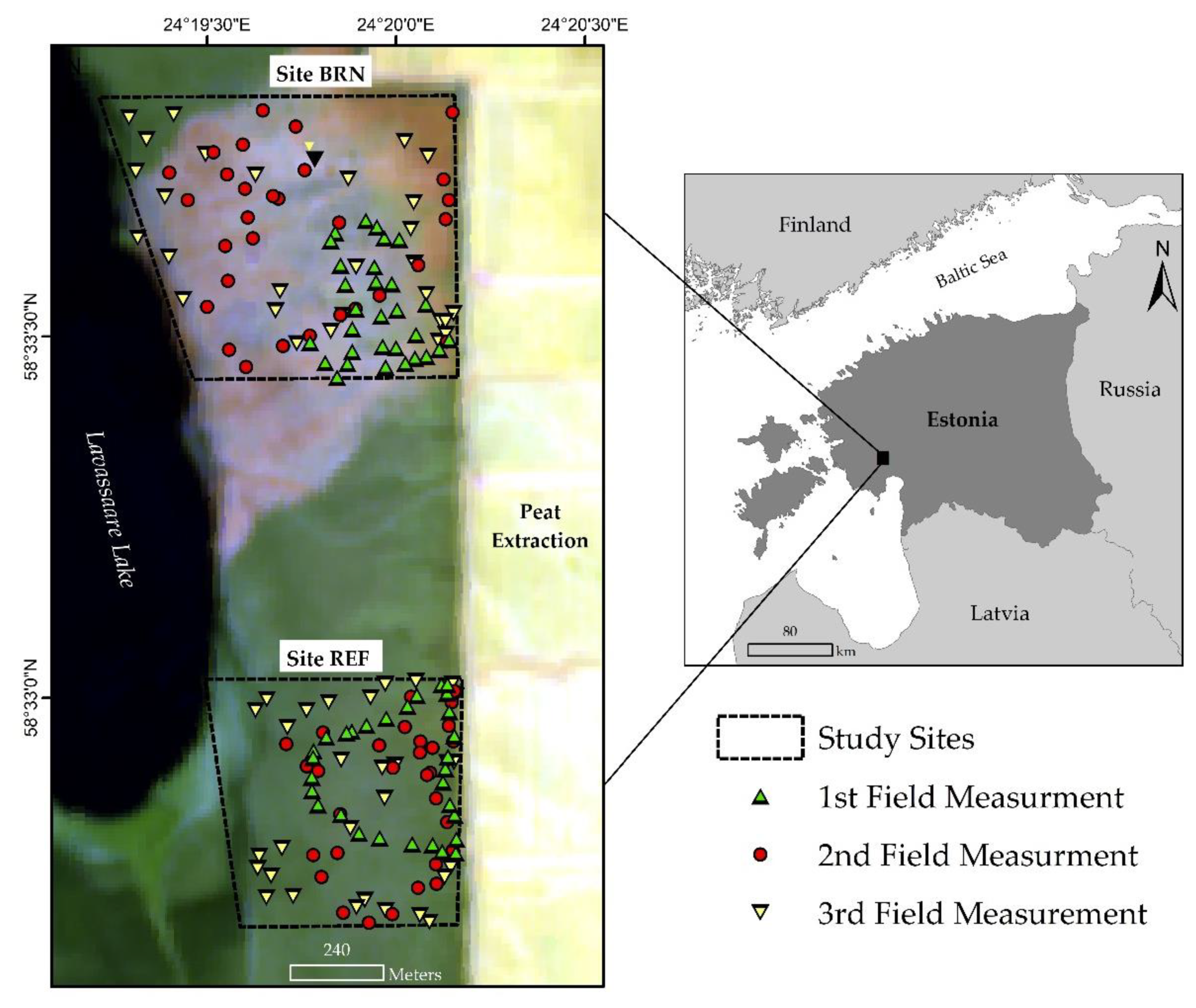
2. Study Area

The study area focused on two sites within the Lavassaare Nature Reserve (Pärnu County, West Estonia, Figure 1). A fire that started on 31 May 2020 from a peat extraction field, spreading in direction to Lake Lavassaare and burning approximately 87 ha, affected the northern location. In total, study sites had an area of 95 hectares.

The study area is separated from the peat extraction mining by a peat embankment 10 to 15 m wide. The thickness of the peat layer in the area is reported to be 0.5 to 1.4 m, composed mainly of Sphagnum angustifolium (Russ.) C. Jens., S. magellanicum Bridel., and S. rubellum Wilson. The height of the water table varies seasonally: in the dry season, it ranges between 5 and 15 cm below the surface, and in rainy and snow melting seasons, it varies from 5 to 20 cm above the ground level [46]. The terrain is mostly flat in the study sites (∆h ≈ 4 m). The vegetation in the area is composed of low-moss vegetation with sparse trees and shrubs [46]. A preliminary assessment of the sampling plots showed that vegetation is mostly constituted by the following plant species: Calluna vulgaris (L.) Hull; Rhynchospora alba (L.) Vahl; Andromeda polifolia L.; Rhododendron groenlandicum (Oeder) Kron and Judd; Betula nana L.; B. pubescens Ehrh.; and Pinus sylvestris L.

According to the weather data from the Estonian Meteorological and Hydrological Institute [47], the long-term average annual temperature in Pärnu County was 6.3 °C, varying between −4.5 and 18 °C, and the average annual precipitation was 746 mm (monthly varying between 37 and 83 mm). Previous studies in Estonian wetlands have reported average soil moisture values around 60% [48] and 86% [49]. Ward et al. [48] recorded SM values of approximately 70% in several locations, even observing a super-saturated soil with an SM of 98%.

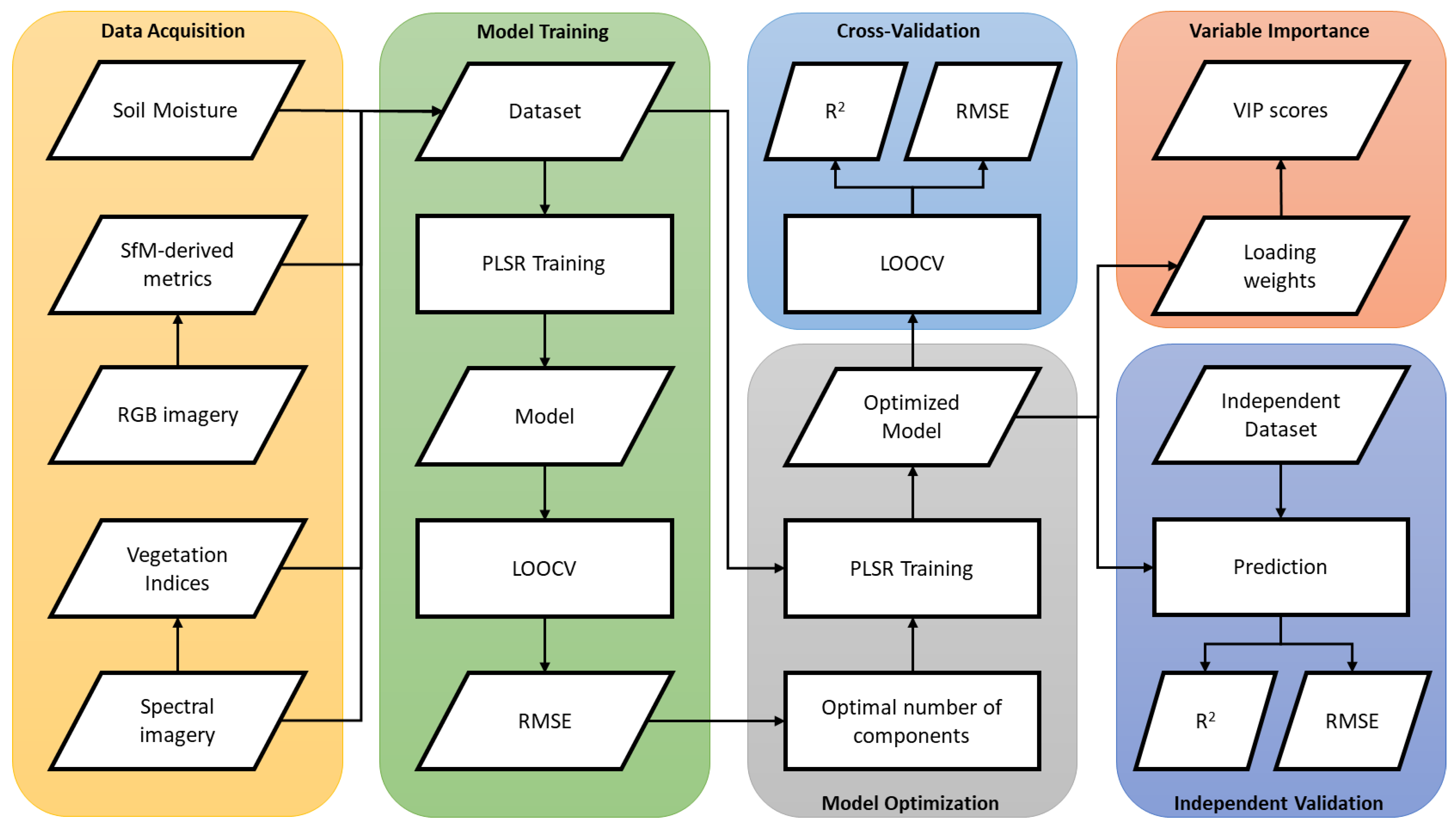
3. Methodology

3.1. Data Acquisition

Three field measurements were conducted in each site: on 16 July 2020 in both sites, on 25 September 2020 in the undamaged site (REF), on 2 October 2020 in the fire-damaged site (BRN), and on 16 May 2021 in both sites. Sample collection followed an unsystematic design (Figure 1) due to site remoteness and difficult accessibility in some regions. In each field sampling campaign, 30 samples per site of soil moisture at 0–10 cm profile were measured using a Delta-T WET Sensor (Delta-T Devices Ltd., London, UK; precision of ±3%) within a 30 × 30 cm quadrat, calculated from the average of three records per sample. The WET sensor calculates the volumetric water content in the soil, which is the ratio between the weight of water and the solids in a given mass of soil sample, and therefore retrieves measurements of soil moisture as a percentage [48,49,50]. We used the manufacturer-suggested parameters for organic soil since it returns similar values to using media-specific calibration [51]. The X, Y, and Z coordinates were recorded within all quadrats using a Trimble R10 dGPS (Trimble, Sunnyvale, CA, USA). Additionally, aboveground biomass (AGB) samples of vascular plants were collected within the quadrat in order to describe the extent of vegetation cover at the sites; however, this variable was not included in the modelling.

Digital images were taken using a fixed-wing eBee X (SenseFly, Cheseaux-sur-Lausanne, Switzerland) equipped with a Sensor Optimized for Drone Applications (SODA), and a Parrot Sequoia in individual acquisition flights. The SODA is designed for photogrammetric analysis and has the following settings: 20 megapixels; global shutter from 1/30 s to 1/2000 s; 10.6 mm focal length; ISO range 125–6400; and exposure compensation in ±2 steps increments. The Parrot Sequoia sensor retrieves 4 distinct 1.2-megapixel spectral bands: green (530–570 nm); red (640–680 nm); red-edge (REG; 730–740 nm); and near-infrared (NIR; 770–810 nm). Flight planning, operation, and post-processing were performed on eMotion Release 3.16.0 (SenseFly, Cheseaux-sur-Lausanne, Switzerland), which enables the operation of autonomous flight missions and post-processing. Flights using SODA camera were set using the following parameters: expected spatial resolution of 3.5 cm/pixel; 80% lateral overlap; and 90% longitudinal overlap. On the other hand, multispectral flights with Parrot Sequoia were set using the following parameters: the expected resolution of 10 cm/pixel; 65% lateral overlap; and 80% longitudinal overlap. Moreover, flights were planned along parallel lines with inclination from north-south direction; with minor on-site adjustment for wind direction before the flight to ensure consistency in image capture spacing, motion blur, and to reduce impairments on subsequent processing effectiveness. We collected images containing an Airinov white-balance target (Airinov, Paris, France) for radiometric correction before each flight with Parrot Sequoia. The used unmanned aerial system (UAS) platform also had an on-board Global Navigation Satellite System Real-time Kinematic/Post-Processed Kinematic (GNSS RTK/PPK) receiver activated. In this way, data recorded during the flight were post-processed in the software using differential correction data provided by the Estonian Land Board’s virtual reference stations [52]. The choice for this approach is based on Tomaštík et al.’s [53] findings, who reported higher horizontal and vertical accuracies using PPK than using ground control points. In addition, multispectral images were taken on the same date as the soil moisture (SM) measurements to ensure that moisture conditions in both soil and vegetation were the same as the field measurements. Further details about flight missions and weather conditions are presented in

Table 1. Summary of imagery acquisition schedule and meteorological conditions during the UAS flights, according to the Estonian Meteorological and Hydrological Institute [47].

Date	7-Day Rainfall Accumulation (mm)	Average Air Temperature (°C)	Average Relative Humidity (%)	Sensor	Site	Starting Time (UTC)
16 July 2020	2.6	18.7	60	SODA	BRN	7:50
				Sequoia	BRN	8:53
				SODA	REF	12:57
				Sequoia	REF	13:36
25 September 2020	5.9	17.9	79	SODA	BRN	8:44
				SODA	REF	9:36
				Sequoia	REF	10:58
2 October 2020	0.2	12.9	70	Sequoia	BRN	8:09
16 May 2021	0.6	13.7	76	Sequoia	BRN	6:50
				SODA	BRN	7:31
				SODA	REF	11:36
				Sequoia	REF	12:11

BRN = the area damaged by the fire, REF = the undamaged area, and UTC = universal time coordinated.

.

3.2. Data Processing

We executed distinct workflows for processing the UAS images to generate 3D dense point clouds and reflectance maps using the software Pix4D Mapper v. 4.3.27 (Pix4D, Lausanne, Switzerland). To process the S.O.D.A dataset and generate the 3D point clouds, we set a full tie-point image scale for initial processing, high point density, a minimum of three tie-points per processed image, and point densification based on half of the image scale. The high-density option for this task was chosen to minimize the occurrence of occlusions in scene reconstruction and reduce data variability in the outputs [54,55]. To process the Parrot Sequoia images and generate reflectance maps, we set a full tie-point image scale, a target for 10,000 keypoints and geometrical verification of matches for initial processing, an optimal point density, a minimum of three tie-points per processed image, and radiometric calibration using the collected images with the Airnov target for camera, solar irradiance, and sun angle correction.

The 3D dense point clouds were classified using the cloth simulation filtering algorithm within the CloudCompare [56] interface. In such a way, points were classified as either ground or off-ground. Based on visual inspection, we applied the following parameters: “Relief” option, disabled slope processing, and set the cloth resolution to 1 m and classification threshold to 0.1. Subsequently, the classified point clouds were processed using the “lidR” [57] package for R software [58]. Initially, we generated digital terrain models (DTM) using a triangulated irregular network interpolator to the ground points at a spatial resolution of 15 cm. The DTMs were used for point clouds’ height normalization and calculation of the following models and metrics: canopy height model (CHM), mean height, median height, range, interquartile range (IQR), standard deviation (SD), and height at the 95th, 90th, 85th, 80th, and 75th percentiles of height distribution (ZQ95, ZQ90, ZQ85, ZQ80, and ZQ75, respectively). Additionally, DTMs were also used to calculate a set of topographical indices to describe microtopographic heterogeneity related to overland water flow (based on the findings of Moser et al. [59]); using SAGA GIS’s [60] tools, we calculated the convergence index (CI), terrain ruggedness index (TRI), length-slope factor (LS), and topographic wetness index (TWI) using default parameters. All point cloud-based metrics were generated at 15 cm spatial resolution.

Lastly, vegetation indices were calculated using reflectance maps generated from the radiometrically corrected Parrot Sequoia imagery;

Table 2. List of vegetation indices used in the present study as input variables in the partial least squares regression models for predicting soil moisture.

Vegetation Index	Equation	Reference
Normalized difference vegetation index (NDVI)	(ρNIR − ρRED)/(ρNIR + ρRED)	[32]
Green normalized difference vegetation index (GNDVI)	(ρNIR − ρGREEN)/(ρNIR + ρGREEN)	[30]
Simple ratio (SR)	ρNIR/ρRED	[61]
Green difference index (GDI)	ρNIR − ρRED + ρGREEN	[62]
Green red difference index (GRDI)	(ρGREEN − ρRED)/(ρGREEN + ρRED)	[62]
Red-edge simple ratio (SRRE)	ρNIR/ρREG	[63]
DATT4	ρRED/(ρGREEN × ρREG)	[64]
Red-edge greenness vegetation index (REGVI)	(ρREG − ρGREEN)/(ρREG + ρGREEN)	[65]
Red-edge vegetation stress index (RVSI)	((ρRED + ρNIR)/2) − ρREG	[66]

ρ_NIR refers to the reflectance at the near-infrared waveband, ρ_RED refers to the reflectance at the red waveband, ρ_GREEN refers to the reflectance at the green waveband, and ρ_REG refers to the reflectance at the red-edge waveband.

summarizes the spectral indices used in this study. We selected these indices considering the varying degrees of vegetation and water stress conditions, as well as the suitability with Parrot Sequoia multispectral bands. Therefore, we used both reflectance maps of the spectral bands (RED, NIR, GREEN, and REG) and vegetation indices as explanatory variables. Spectral metrics were also generated at the spatial resolution of 15 cm.

3.3. Statistical Analyses

We grouped the samples within 11 datasets according to the sites and field measurement dates; these datasets were described in

Table 3. Description of the datasets used for predicting soil moisture and their respective sample size.

Dataset		Sites	Dates	Training Samples (n)
Specific	BRN1	BRN	16 July 2020	30
	BRN2		2 October 2020	30
	BRN3		16 May 2021	30
	REF1	REF	16 July 2020	30
	REF2		25 September 2020	30
	REF3		16 May 2021	30
Date-merged	DAY1	BRN + REF	16 July 2020	60
	DAY2		25 September 2020 + 2 October 2020	60
	DAY3		16 May 2021	60
Site-merged	BRNALL	BRN	16 July 2020 + 2 October 2020 + 16 May 2021	90
	REFALL	REF	16 July 2020 + 25 September 2020 + 16 May 2021	90

BRN = the area damaged by the fire, REF = the undamaged area.

. We performed an exploratory data analysis using Spearman’s correlation coefficient (r) to assess relationships, and coefficient of variation (CV) to describe the magnitude of variability across SM, spectral, and Structure-from-Motion (SfM) derived metrics. Moreover, Figure 2 presents a simplified illustration of the workflow for the partial least squares regression (PLSR) modelling used in this study.

For this purpose, we fitted PLSR models in R [58] using package “pls” [67]. A priori, all pixels within each sample quadrat were assigned to their respective average SM from the field measurements. We also scaled the variables to zero mean and unit variance. In the first training step, the models for predicting SM used all the SfM-derived metrics and vegetation indices calculated in previous steps as explanatory variables, which generated 28 potential latent variables. We assessed the performance of models using a different number of components by using a leave-one-out cross-validation (LOOCV) procedure [68,69]. Considering the root-mean-squared error of the predictions (RMSE; Equation (1)), we chose the optimal model size based on Mevik and Cederkvist’s [70] approach. The RMSE allows the comparison between datasets and models with different ranges of predicted values and provides an unbiased indicator of prediction error. In such a way, we selected the model with one dimension less than the model with the smallest RMSE, which provides a simpler and operationally improved alternative model that reduces data dimensionality and overfitting issues [70]. Subsequently, we fitted the optimized models using a reduced number of components, which were then assessed, validated, and discussed. Supplementary Material S1 provides the specification files for each model fitted in the present study; these files can be loaded into R software for further applications.

$$\mathrm{RMSE}=\frac{1}{n}\sqrt{{\displaystyle \sum }{\left(y_i-\overline{y}\right)}^2}$$

(1)

where: n = number of observations, $y_i$ = observation i value of the prediction, and $\overline{y}$ = mean value of observations.

To assess the importance of variables for modelling the SM, we calculated the variable influence in projection (VIP) scores. The VIP score provides estimations of the contribution of each predictor to the model based on the correlation with the response variable and the variance explained by the latent variables [71]. For this purpose, we used the R-package “plsVarSel” [71], which provides interfaces and methods for supporting variable selection within PLSR frameworks. This package uses Equation (2) for calculating the VIP scores. According to Galindo-Prieto et al. [72], VIP values greater than 1 indicate the most relevant variables, while VIP values less than 0.5 are considered irrelevant in the model.

$$\mathrm{VIP}=\sqrt{{\displaystyle \sum }\left[S{S}_a\left(w_{aj}/\left|\right|w_a\left|\right|{}^2\right)\right]/{\displaystyle \sum }S{S}_a}$$

(2)

where: $S{S}_a$ = sum of squares explained by the ath dimension (i.e., latent variable); $w_{aj}$ = the loading weight of the jth variable at the ath dimension; and $w_a$ = the loading weight of the ath dimension.

In addition to the cross-validation procedure, we assessed the performance of models when applied to independent datasets to evaluate the transferability potential across dates and sites. To illustrate the independent validation, the SM values for site REF on the first measurement date (i.e., REF1 dataset) were predicted using the models trained using the datasets REF2, REF3, BRN1, BRN2, BRN3, etc. For this, we took into account the RMSE as well as the coefficient of determination (R²) of the fitting between predicted and observed SM values. Lastly, we considered values smaller than 0.50 weak model fit, values between 0.50 and 0.75 as moderate fit, and values larger than 0.75 as a good fit.

4. Results

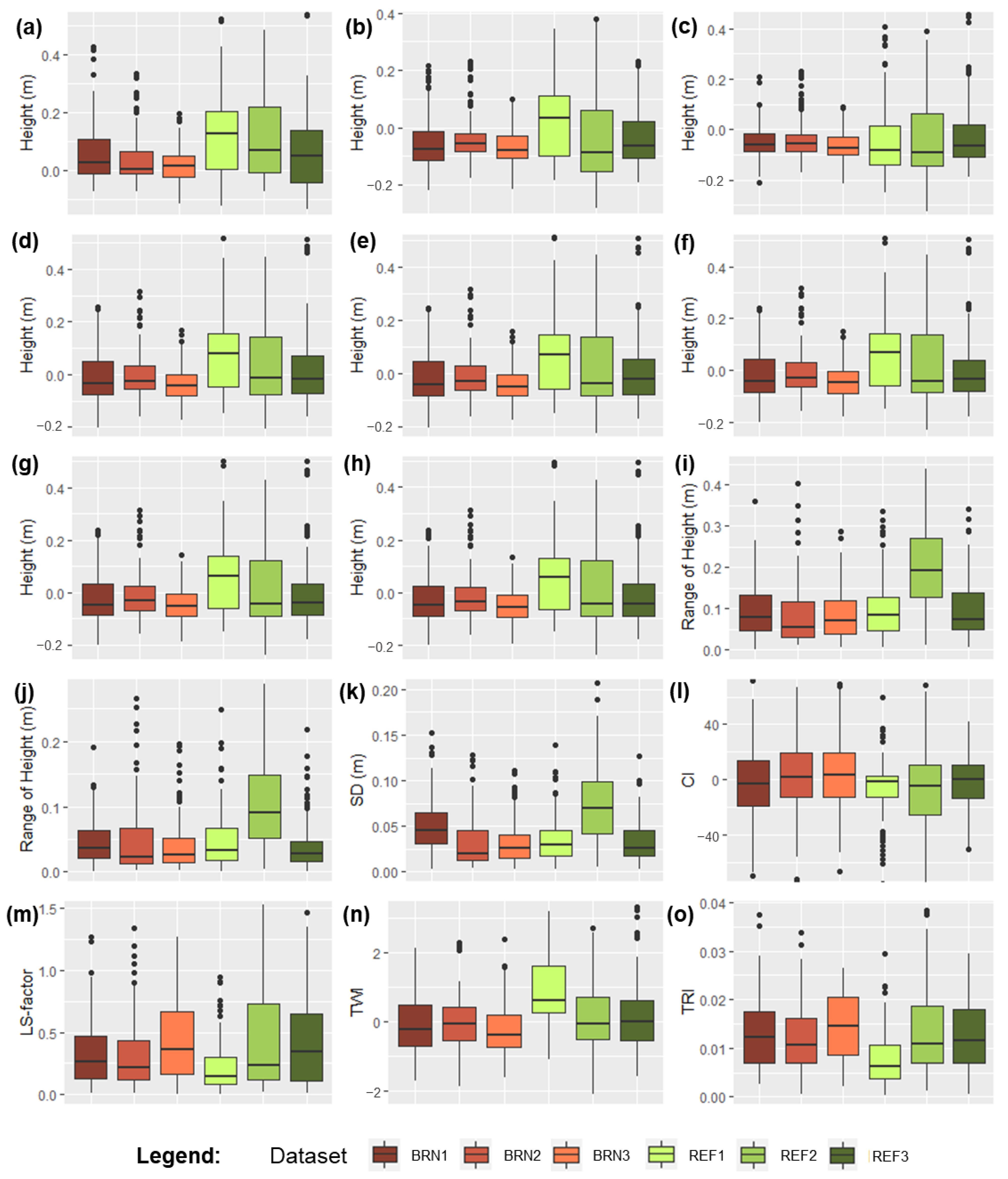
4.1. Description of the Sampled Data

We present the summarized soil moisture (SM), aboveground biomass (AGB), spectral (Figure 3), and Structure-from-Motion (SfM)-derived data (Figure 4) for the 1st, 2nd, and 3rd dates of field measurements for both sites. The SM values ranged from 9.5% and 88.2% along with the study (Figure 3a). The undisturbed site (REF) consistently had higher SM values than the fire-damaged site (BRN). Figure 3a shows that SM values varied mostly between 20 and 75%. In this context, the observed values in the present study seem to agree with the values reported in the literature for wetlands in different biomes [18,48,49]. Considering SM’s coefficient of variation (CV) within quartiles of sample distributions, no obvious pattern manifested. In site BRN, the upper interval of values (i.e., above the 4th quartile) had high CV values; 15.76%, 22.87%, and 28.54% for BRN1, BRN2, and BRN3, respectively. On the other hand, the lowest quartiles (i.e., below the 1st quartile) had variability in site REF. In these intervals, CV values were 21.38%, 44.04%, and 25.43% for BRN1, BRN2, and BRN3, respectively. Regarding the AGB, it varied between 44.4 and 79.6 g/m² at site BRN and between 278.8 and 357.2 g/m² at site REF. Among the spectral metrics, the NDVI had high variability within the lowest quartiles, ranging from 9.56% (below the first quartile of REF3) to 20.46% (below the 1st quartile of BRN2). Furthermore, RVSI showed high CV values within quartiles, with a maximum observed CV of 175% in the 4th quartile of BRN2.

Moreover, the correlation matrix diagrams from the exploratory data analysis (Figure 5) showed that SM had moderate, negative correlations with SfM-derived and topographic metrics. The spectral-derived metrics were often positively correlated with SM in site REF. For example, RVSI and DATT4 had correlation coefficients of 0.62 and 0.60, respectively, with SM in the second measurement date. On the other hand, we observed a negative correlation of SM with NDVI (−0.74), SR (−0.74), and GRDI (−0.68). SM had a negative relation with the AGB in site REF, with r varying between −0.69 and −0.48. In site BRN, this relation was changeable across dates (−0.69–0.28). The correlation diagrams also indicated the predictors were highly interrelated within their groups (i.e., spectral, height-related, and topographic metrics), especially the SfM-derived metrics concerning height values. Considering the relation between these groups, we observed a stable pattern at site BRN, with slight variations in the magnitude of correlations. Contrarily, the relationship between some variables changed between dates. For example, the monochromatic bands (i.e., RED, GREEN, NIR, and REG) had both positive and negative correlations with height metrics in the first measurement (Figure 5a), only positive in the second (Figure 5b), and only negative in the third (Figure 5c).

4.2. Model Performance according to the Empirical Datasets

Considering the performance of the models for explaining the empirical datasets, RMSE values for models trained and optimized with BRN1 and REF1 datasets were 13.08% and 13.29%, respectively. The optimization procedure reduced the number of dimensions of these models to 18 and 13 for BRN1 and REF1, respectively. Based on the LOOCV procedure, the R² values for these models were 0.700 and 0.725. For BRN2 and REF2, the RMSE values were 13.87% and 14.44%, respectively; R² for these models were 0.577 and 0.553, respectively. The optimal number of dimensions for BRN2 was 27 and for REF2 was 14. In the third measurement round, the model trained using BRN3 had an R² of 0.467, while the model using REF3 showed an R² of 0.668. The RMSE and the optimal number of dimensions were 14.81% and 7 for BRN3, and 19.21% and 11 for REF3. When considering date-merged datasets, the model DAY1 had an RMSE of 15.99% and an R² of 0.586. The model using the DAY2 dataset had an RMSE of 17.48% and an R² of 0.520. For model DAY3, the metrics were 18.23% and 0.203, respectively. The optimal number of dimensions for these models were 11, 19, and 13. Considering the site-merged datasets, the RMSE was 17.44% and the R² was 0.316 for the model using the BRN_ALL dataset; for REF_ALL, the values were 18.94% and 0.443, respectively. These models included 19 and 14 dimensions, respectively.

Supplementary Material S2 provides the complete set of loadings for each model. Considering the main latent variables obtained from the partial least squares regression (PLSR) models, we observed that dimensions representing gradients of plant health and biomass amount were the most frequent among models. For example, model BRN1’s three major dimensions reproduce plant status gradients, accounting for 58.6% of SM’s explained variability. Similarly, the most relevant dimensions in model DAY1 were related to health and vegetation cover gradients (48.2%). Furthermore, representations of physical gradients were common, particularly in models related to the REF site and merged models. Among these models, the main dimensions related to microtopography accounted for 4.3% (i.e., REF_ALL) to 20.0% (i.e., DAY2) of SM’s variability. The VIP scores revealed distinct patterns of variable importance across sites (Figure 6). For example, on the REF site, both predictor types were the most relevant for model construction (i.e., VIP > 1.0). The exception was model REF2, in which most of the relevant predictors were spectral-based. On the other hand, the most influential predictor type was changeable across specific datasets in the BRN site. Both types were relevant in the first measurement date (i.e., BRN1). On the second date (i.e., BRN2), the SfM-derived metrics had greater importance, while the spectral metrics were more important on the last date (i.e., BRN3). Finally, the date-merged models showed a similar pattern of variable importance. The SfM-derived metrics were more relevant on the first date (i.e., DAY1), while the spectral-derived indices were more expressive on the third date (i.e., DAY3).

4.3. Model Assessment Using the Validation Datasets

The assessment of PLSR model performance against independent datasets showed reduced potential for spatial and temporal transferability, especially for BRN datasets. As shown in Figure 7 and Figure 8, we observed that the models that included site-specific samples outperformed those using fully independent samples. This condition was more evident for predicting BRN datasets (Figure 7). The fully independent models could only explain up to 17% of the data variability in these datasets; the RMSE of these models ranged from 16.1% to 23.9%. On the other hand, models that included the original datasets had moderate to good performance (RMSE < 16.7%, and R² > 0.52), and exceptions were for the dataset BRN3 (RMSE > 14.3%, and R² < 0.29).

Comparing with site BRN, the performance of independent models improved slightly on the REF site (Figure 8). In this way, some models that used training samples from the REF but different dates achieved moderate prediction ability. For example, using model REF2 to predict the REF1 dataset resulted in an RMSE of 16.3% and an R² of 0.59. Furthermore, including training samples from external sites improved prediction accuracy, especially when collected simultaneously. For instance, for the REF3 dataset, both date- and site-merged models had greater accuracy than the site-specific model. However, the overall model performance for this dataset was poor; these models could explain up to 33% of the data variability, and the minimum RMSE was 18.6% for this dataset. Lastly, Supplementary Material S3 provides the spatial prediction maps of the best performance models for each site and measurement date.

5. Discussion

5.1. Models’ Ability for Predicting Soil Moisture Using Remote Sensing Optical Data

Overall, our partial least squares regression (PLSR) models had a limited ability to describe the relationship between soil moisture (SM) and environmental factors, with weak to moderate explanatory power (i.e., 0.29 < R² < 0.73). Other studies predicting soil moisture had comparable findings with our upper limits. For example, Araya et al. [25] predicted SM with an MAE of 3.8% and R² of 0.71 using decision-tree-based models and multispectral reflectance, terrain variables, rainfall, and potential evapotranspiration as predictors. Amani et al. [27] obtained correlation coefficients varying between −0.65 and −0.34 with field-measured soil moisture values, comparing different satellite-based dryness indices and including thermal datasets. Furthermore, Wigmore et al. [18] had R² between 0.55 and 0.76 using the triangular feature calculated from the relation between surface temperature and NDVI (i.e., temperature-vegetation dryness index (TVDI)) predicted from unmanned aerial system (UAS) data. Considering non-linear relationships, Hajdu et al. [28] modelled SM using synthetic aperture radar metrics, topography, season, and NDVI as predictors and obtained an R² of 0.86 using random forests (RF) models. Similarly, Sharma et al. [11] observed a high explanation ability for predicting soil moisture from NDVI using a logistic model (R² = 0.83). Altogether, the accuracy verified for our models was equivalent to other UAS-based models [18,23,25,73] and satellite-based models [27,28,74,75], especially at the first two measurement dates (i.e., BRN1, BRN2, REF1, REF2, DAY1, and DAY2).

In this regard, the literature shows that approaches assuming non-linearity achieved better performance than linear relationships for predicting SM as a function of remote sensing (RS) data. Machine learning techniques such as random forests [76] could handle these complex relationships, improving the performance of predictive models [25,28]. However, to ensure unbiased and meaningful predictions, these techniques require relatively large datasets for model training [25,77], possibly compromising the feasibility of operationalizing a framework such as this. Aside from that, some of these methods are considered black-box techniques, providing limited information about relationships between inputs and outputs [25]. For this reason, PLSR emerges as a promising alternative for SM prediction using RS data. It provides a practical framework for dealing with datasets with a small sample size but a large number of correlated predictor variables [43]. Furthermore, it provides reliable and consistent outputs for determining the magnitude of variable influence and selecting relevant predictors, which improves understanding of underlying phenomena [43].

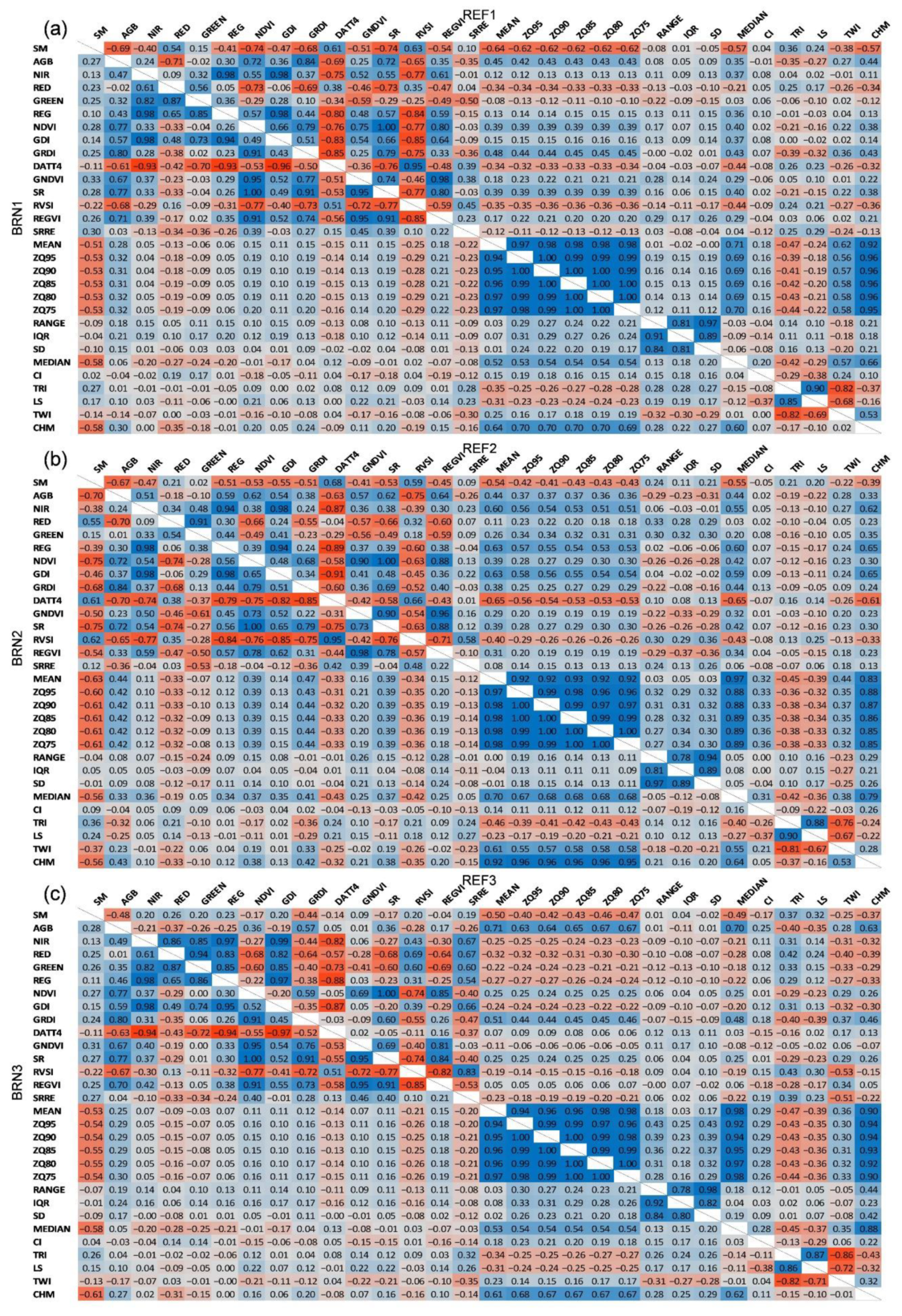
5.2. The Explanatory Importance of Spectral and SfM-Derived Datasets for Predicting Soil Moisture

Our results indicated that the importance of spectral and Structure-from-Motion (SfM)-derived metrics depends on a combination of environmental factors. In such a way, this finding may suggest that SfM-derived metrics are the best predictors for representing soil moisture over exposed surfaces, given the lesser vegetation cover in the area damaged by the fire (i.e., site BRN) at the beginning of the monitoring period. It implies that these models captured the influence of differences in microtopography on soil moisture, especially on those dates closer to the fire event. Other studies verified the influence of microtopographic features on SM moisture gradients in wetlands [59,78]. From this perspective, our findings agree with Enwright et al. [79] who observed increased uncertainty of terrain modelling under herbaceous and shrub vegetation cover. In addition, Moore et al. [33] stated that vegetation cover also reduces the relative importance of peatland geomorphology on soil heating and ecosystem fluxes, consequently affecting local hydrological fluxes [20,80].

In addition to SfM metrics, the consistent importance of spectral metrics for models derived from the undamaged area (i.e., site REF) datasets suggests that vegetation indices may be adequate to describe the plant health conditions associated with water stress. The literature supports the significance of NDVI for this representation as this index is widely applied to assess vegetation’s greenness and photosynthetic activity, cover fraction, and status [11,31,32,74]. Low values of this index may also indicate disturbed conditions in our study area, such as exposed surfaces or desiccated vegetation [29]. Besides this, the RVSI’s relevance to the models is also consistent with the literature; Perry and Roberts [81] observed that NIR-based indices are sensitive to water content. For the model REF_ALL, GRDI and DATT had the highest VIP scores. In this regard, some studies [65,82,83,84] verified that red-edge and near-infrared spectral indices describe plant health and water stress. For example, Fernández-Manso et al. [85] observed that the red-edge reflectance is sensitive to different degrees of burn severity, thus describing conditions of chlorophyll content, vegetation cover, and soil moisture.

Lastly, the PLSR dimensions also indicated that vegetation status patterns were the most influential on SM variability on the first measurement date, particularly for the dataset BRN1. This finding agrees with Kettridge et al. [86], who observed increased water repellency caused by wildfire disturbance in a peatland. In such a way, it may indicate that the differences between disturbed and undisturbed vegetation have the highest association with the moisture conditions in site BRN, especially immediately after the fire. Furthermore, Lendzioch et al. [36] observed that vegetation cover plays a critical role in microclimate regulation of the soil surface, influencing temperature and thus moisture content. On the other hand, topographical gradients were more important at the REF site due to its homogeneous vegetation cover. Under these conditions, the micro-topographical features most likely control the additional variability in SM. These features influence the water distribution and availability in peatlands through different mechanisms, such as the exposure of the water table [80] or the preferential routing of runoff [20,59].

Altogether, the observed factor relevance switch from SfM-derived metrics in the first measurements to spectral metrics in the last field observation might reflect the effect of vegetation regrowth on the surface coverage [87] after the fire event as well as differences in humidity conditions among measurement days. This finding is consistent with Fatichi et al. [17] and Srivastava et al. [20]. The authors verified that the relative importance of biotic and abiotic factors varied along the year according to humidity conditions, following a hysteresis pattern (i.e., the differential relationship between soil water content and potential during wetting and drying processes). In this regard, Srivastava et al. [20] verified that vegetation is more influential on the temporal variability of SM, while topography is more strongly related to the spatial pattern. Thus, our results present a similar pattern: spectral metrics were more relevant in models merging different dates (i.e., BRN_ALL, REF_ALL), and SfM-derived metrics were often more relevant in models merging different sites within the same date (i.e., DAY1, DAY2, and DAY3).

5.3. The Transferability of Models across Dates and Sites

The assessment of the transferability potential of PLSR models showed unsatisfactory results, especially for site BRN. The poor performance of merged models is consistent with Millard et al. [21]. They verified that linear mixed-effect models were inefficient for predicting SM at dates not used in the training step in a temporally homogeneous grassland community; in their case, R² was less than 0.3. Both findings can be attributed to an incomplete representation of the lower and upper regions of the SM gradient spectrum, which are typically poorly described within empirical datasets [19], resulting in increased uncertainties in predictions within these intervals. In this regard, acquiring samples on different ranges of SM variability is beneficial for constructing more robust and reliable models [17,21,25].

Besides that, the low accuracy achieved at site BRN may indicate that model performance may be affected by changes in vegetation cover. As discussed, vegetation regrowth since the fire event seems to be switching the importance of the major indices and their explanatory ability, following the hysteresis pattern described by Fatichi et al. [17]. In this regard, independent models performed worse than others due to both the weaker correlations between SM and VIs in low vegetation cover and the limitation of VIs to describe immediate responses of the plant health caused by drought [1,7,24]. West et al. [29] observed that a certain level of vegetation cover (i.e., 30–40%) is necessary to detect these correlations. Given its increased vegetation cover and biomass, this threshold would explain the slightly better potential for transferability at site REF.

5.4. Implications for UAS-Based Soil Moisture Modeling and Monitoring, and Limitations in This Study

The use of PLSR models to predict SM using optical RS data proved that the method’s outputs could be used to identify underlying patterns and variables of interest. As mentioned, Ainiwaer et al. [44] could identify the most relevant wavelengths for predicting SM from a hyperspectral dataset using PLSR. As a result, the loading weights supported the determination of the optimum wavelengths for their purpose. In this perspective, better interpretability of the model’s output is a critical aspect in establishing functional linkages between variables with a biological or physical meaning [43]. Furthermore, it has been demonstrated that the weights of indicators produced by this method are robust independent of sample size [42]. Additionally, the effect of vegetation heterogeneity illustrated by the results highlights the role of choosing the appropriate variables to ensure accurate results from optical UAS data. Thus, it appears to be a suitable method for evaluating and monitoring SM. The main disadvantage of this method is that it employs linear combinations of multidimensional space of predictor variables [88], which may oversimplify the description of those relationships. The improvement in spatial resolution promoted by UAS-based methods offers a better understanding of fine-scale processes related to SM and modelling microtopographical features at appropriate spatial scales, which vary in small horizontal and vertical scales (0.2–10 m) [33], and thus satellite-based models usually fail to represent them due to the coarse resolution of their sensors [18]. In such a way, our findings illustrated the limitations of optical remote sensing to predict SM due to the complex relationship (i.e., non-linear) between this variable, surface temperature, and plant physiology [2,19,24].

Lastly, it is worth mentioning that the study might have presented some limitations regarding the sample design. The small sample size for training the models likely impaired their performances. In this way, increasing sample sizes would improve the accuracy of predictions and allow the retrieval more robust validations. In addition, the unsystematic sampling design across the dates due to accessibility reasons might have affected the representativeness of the whole area. However, this issue could be addressed by splitting the study sites into sub-blocks and increasing the sample size to smaller extents. It would contribute to the statistical replication of models, providing a better understanding of model performance and factors affecting the framework. In this context, the integration of both spectral and SfM-derived metrics would counterbalance the drawbacks of each type of data, and they might be complementary for SM monitoring over homogenous vegetation cover. The uncertainties related to optical RS methods remain the main challenge for exploiting the full potential of SM predictions in hydrological applications. To reduce them, carrying out a priori mappings of the land cover would guide and optimize data collection and also reduce the risks of diminishing the importance of specific variables [29]. For this reason, we recommend structuring fieldwork campaigns to account for probable SM value extremes occurring within the study area based on early evaluations or previous reports from the same place. Besides increasing model complexity, it is worth noting that using ancillary data and covariates can improve model fitting by introducing weather, season, or site-specific information to the models that are not present in the training data [21]. Hence, the inclusion of surface temperature [36], meteorological variables, or vegetation cover [19], for example, can improve the accuracy of our SM predictions.

6. Conclusions

This study demonstrated a conditional suitability of soil moisture (SM) modelling from optical unmanned aerial system (UAS) data and provided general insights for future research and applications across time and sites. More specifically, we used partial least squares regression (PLSR) models to predict soil moisture from optical data acquired by UAS. According to the previously defined objectives, our results demonstrated that:

(1)

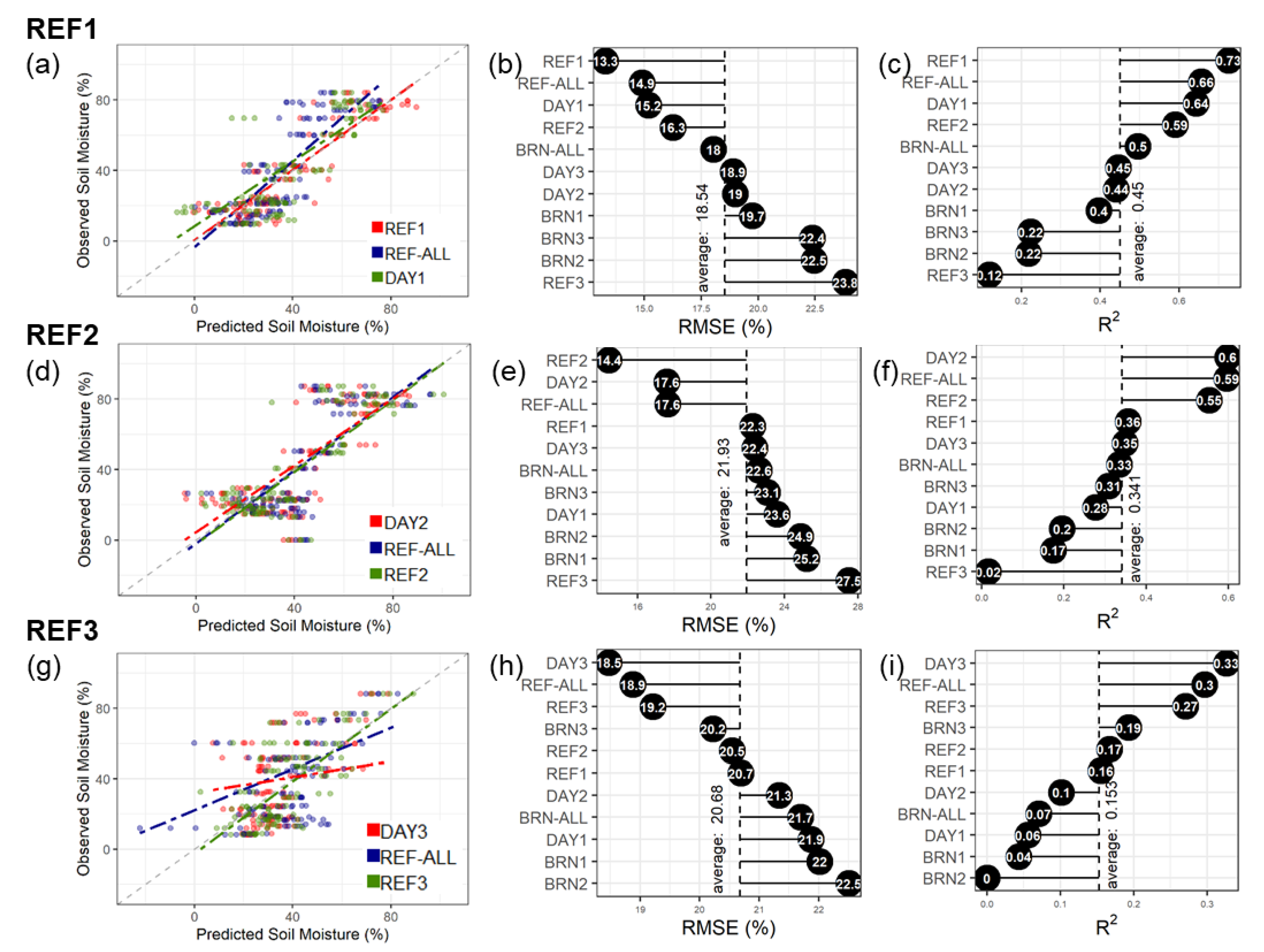
Microtopography and vegetation characteristics influenced SM. Following the effects of the wildfire on vegetation cover, plant health gradients had a higher influence on SM variability in the early phases of vegetation regeneration (e.g., BRN1 and DAY1). Similarly, individual SfM-derived metrics in this site had decreasing relevance over the monitoring period, with strong effect in models during the first two measurement dates (i.e., datasets BRN1 and BRN2), illustrating the influence of vegetation growth on the mechanisms of soil water distribution. On the other hand, physical gradients were more influential in more homogeneous conditions (i.e., site REF and date-merged datasets), illustrating its influence on SM spatial variability;

(2)

The performance of the partial least squares regression (PLSR) models based on optical data—namely spectral and SfM-derived metrics—was moderate but comparable with techniques (i.e., microwave and satellite-based) that are more complex and expensive. Compared to satellite-based approaches, UASs retrieve data at appropriate resolutions, allowing observation of processes and dynamics related to SM. As a result, these approaches may be able to overcome the impaired explanatory ability of satellite-borne sensors caused by their coarser spatial resolution;

(3)

A dominance of SfM-derived metrics for predictions over exposed surfaces. The application of theses metrics for monitoring SM seems to be a promising and effective alternative for evaluating the spatial distribution of SM over these surfaces. Thus, it suggests that a single, low-cost, and consumer-grade camera should be sufficient for rapid assessment at these sites. Moreover, it demonstrates that the spectral metrics might be meaningful proxies for providing indirect measures of temporal variation of moisture conditions, which explains the improved prediction accuracy of these models for REF datasets, even using external samples. In this situation, frameworks comprising two sensors could be appropriate for predicting SM in relatively preserved and uniformly vegetated environments; and

(4)

The models had unsatisfactory applicability across dates and places, particularly in highly heterogeneous locations. The best results in this regard were observed at the REF site, where vegetation structure was temporally and spatially more stable. Under those conditions, extra samples from different areas and time frames would likely improve prediction accuracy. Increasing the sample size to include the full range of SM values can reduce the uncertainties caused by the complexity of SM relationships. Therefore, we recommend developing specific models or carrying out field measurements of SM in every monitoring step to include in merged models.

Overall, the moderate accuracy achieved in this study suggests that integrating UAS data with PLSR models is a suitable framework for modelling SM at a fine resolution, particularly because its increased interpretability appears to offset the limitations of linear representation. The results showed that visible wavelength indices provided useful information for SM modelling. Many optical RS applications rely on non-visible wavelengths, which, although providing better performance, are more difficult and expensive to obtain. We showed its feasibility for retrieving SM in field-scale investigations, encouraging an improved cost-benefit ratio for short-term monitoring. It may reduce the need for more complex, resource-consuming information (i.e., active RS approaches and ancillary data) and benefit the application of resources and time flexibility for monitoring tasks. Further research should focus on testing the methodology, including new indices and data sources (e.g., temperature, weather, or site-related).

References

- Ahmed, M.; Else, B.; Eklundh, L.; Ardö, J.; Seaquist, J. Dynamic response of NDVI to soil moisture variations during different hydrological regimes in the sahel region. Int. J. Remote Sens. 2017, 38, 5408–5429. [Google Scholar] [CrossRef]
- Wang, L.; Qu, J.J. Satellite remote sensing applications for surface soil moisture monitoring: A review. Front. Earth Sci. China 2009, 3, 237–247. [Google Scholar] [CrossRef]
- Xu, X.; Zhang, Q.; Tan, Z.; Li, Y.; Wang, X. Effects of water-table depth and soil moisture on plant biomass, diversity, and distribution at a seasonally flooded wetland of Poyang Lake, China. Chin. Geogr. Sci. 2015, 25, 739–756. [Google Scholar] [CrossRef]
- Damm, A.; Paul-Limoges, E.; Haghighi, E.; Simmer, C.; Morsdorf, F.; Schneider, F.D.; van der Tol, C.; Migliavacca, M.; Rascher, U. Remote sensing of plant-water relations: An overview and future perspectives. J. Plant Physiol. 2018, 227, 3–19. [Google Scholar] [CrossRef]
- Liu, L.; Gudmundsson, L.; Hauser, M.; Qin, D.; Li, S.; Seneviratne, S.I. Soil moisture dominates dryness stress on ecosystem production globally. Nat. Commun. 2020, 11, 4892. [Google Scholar] [CrossRef] [PubMed]
- Brocca, L.; Ciabatta, L.; Massari, C.; Camici, S.; Tarpanelli, A. Soil moisture for hydrological applications: Open questions and new opportunities. Water 2017, 9, 140. [Google Scholar] [CrossRef]
- Joiner, J.; Yoshida, Y.; Anderson, M.; Holmes, T.; Hain, C.; Reichle, R.; Koster, R.; Middleton, E.; Zeng, F.W. Global relationships among traditional reflectance vegetation indices (NDVI and NDII), evapotranspiration (ET), and soil moisture variability on weekly timescales. Remote Sens. Environ. 2018, 219, 339–352. [Google Scholar] [CrossRef] [Green Version]
- Orru, M.; Ots, K.; Orru, H. Re-vegetation processes in cutaway peat production fields in Estonia in relation to peat quality and water regime. Environ. Monit. Assess. 2016, 188, 655. [Google Scholar] [CrossRef]
- Fenner, N.; Freeman, C. Drought-induced carbon loss in peatlands. Nat. Geosci. 2011, 4, 895–900. [Google Scholar] [CrossRef]
- Grau-Andrés, R.; Davies, G.M.; Gray, A.; Scott, E.M.; Waldron, S. Fire severity is more sensitive to low fuel moisture content on Calluna heathlands than on peat bogs. Sci. Total Environ. 2018, 616–617, 1261–1269. [Google Scholar] [CrossRef] [Green Version]
- Sharma, S.; Carlson, J.D.; Krueger, E.S.; Engle, D.M.; Twidwell, D.; Fuhlendorf, S.D.; Patrignani, A.; Feng, L.; Ochsner, T.E. Soil moisture as an indicator of growing-season herbaceous fuel moisture and curing rate in grasslands. Int. J. Wildl. Fire 2020, 30, 57–69. [Google Scholar] [CrossRef]
- Kimmel, K.; Mander, Ü. Ecosystem services of peatlands: Implications for restoration. Prog. Phys. Geogr. 2010, 34, 491–514. [Google Scholar] [CrossRef]
- Nijp, J.J.; Metselaar, K.; Limpens, J.; Teutschbein, C.; Peichl, M.; Nilsson, M.B.; Berendse, F.; van der Zee, S.E.A.T.M. Including hydrological self-regulating processes in peatland models: Effects on peatmoss drought projections. Sci. Total Environ. 2017, 580, 1389–1400. [Google Scholar] [CrossRef] [PubMed]
- Davies, G.M.; Legg, C.J. Regional variation in fire weather controls the reported occurrence of Scottish wildfires. PeerJ 2016, 4, e2649. [Google Scholar] [CrossRef] [PubMed] [Green Version]
- Roulet, N.T.; Lafleur, P.M.; Richard, P.J.H.; Moore, T.R.; Humphreys, E.R.; Bubier, J. Contemporary carbon balance and late Holocene carbon accumulation in a northern peatland. Glob. Chang. Biol. 2007, 13, 397–411. [Google Scholar] [CrossRef] [Green Version]
- Turetsky, M.R.; Donahue, W.F.; Benscoter, B.W. Experimental drying intensifies burning and carbon losses in a northern peatland. Nat. Commun. 2011, 2, 514. [Google Scholar] [CrossRef]
- Fatichi, S.; Katul, G.G.; Ivanov, V.Y.; Pappas, C.; Paschalis, A.; Consolo, A.; Kim, J.; Burlando, P. Abiotic and biotic controls of soil moisture spatiotemporal variability and the occurrence of hysteresis. Water Resour. Res. 2015, 51, 3505–3524. [Google Scholar] [CrossRef]
- Wigmore, O.; Mark, B.; McKenzie, J.; Baraer, M.; Lautz, L. Sub-metre mapping of surface soil moisture in proglacial valleys of the tropical Andes using a multispectral unmanned aerial vehicle. Remote Sens. Environ. 2019, 222, 104–118. [Google Scholar] [CrossRef]
- Rahimzadeh-Bajgiran, P.; Berg, A.A.; Champagne, C.; Omasa, K. Estimation of soil moisture using optical/thermal infrared remote sensing in the Canadian Prairies. ISPRS J. Photogramm. Remote Sens. 2013, 83, 94–103. [Google Scholar] [CrossRef]
- Srivastava, A.; Saco, P.M.; Rodriguez, J.F.; Kumari, N.; Chun, K.P.; Yetemen, O. The role of landscape morphology on soil moisture variability in semi-arid ecosystems. Hydrol. Process. 2021, 35, e13990. [Google Scholar] [CrossRef]
- Millard, K.; Thompson, D.K.; Parisien, M.A.; Richardson, M. Soil moisture monitoring in a temperate peatland using multi-sensor remote sensing and linear mixed effects. Remote Sens. 2018, 10, 903. [Google Scholar] [CrossRef] [Green Version]
- Petropoulos, G.P.; Ireland, G.; Barrett, B. Surface soil moisture retrievals from remote sensing: Current status, products & future trends. Phys. Chem. Earth 2015, 83–84, 36–56. [Google Scholar] [CrossRef]
- Lu, F.; Sun, Y.; Hou, F. Using UAV visible images to estimate the soil moisture of steppe. Water 2020, 12, 2334. [Google Scholar] [CrossRef]
- Zhang, D.; Zhou, G. Estimation of soil moisture from optical and thermal remote sensing: A review. Sensors 2016, 16, 1308. [Google Scholar] [CrossRef] [PubMed] [Green Version]
- Araya, S.N.; Fryjoff-hung, A.; Anderson, A.; Viers, J.H.; Ghezzehei, T.A. Advances in Soil Moisture Retrieval from Multispectral Remote Sensing Using Unmanned Aircraft Systems and Machine Learning Techniques. Hydrol. Earth Syst. Sci. 2021, 25, 2739–2758. [Google Scholar] [CrossRef]
- Senyurek, V.; Farhad, M.; Gurbuz, A.C.; Kurum, M.; Moorhead, R. SoilMoistureMapper: A GNSS-R approach for soil moisture retrieval on UAV. In AI for Agriculture and Food Systems; Association for the Advancement of Artificial Intelligence: Menlo Park, CA, USA, 2021. [Google Scholar]
- Amani, M.; Salehi, B.; Mahdavi, S.; Masjedi, A.; Dehnavi, S. Temperature-Vegetation-soil Moisture Dryness Index (TVMDI). Remote Sens. Environ. 2017, 197, 1–14. [Google Scholar] [CrossRef]
- Hajdu, I.; Yule, I.; Dehghan-shoar, M.H. Modelling of Near-Surface Soil Moisture Using Machine Learning and Multi-Temporal Sentinel 1 Images in New Zealand. In Proceedings of the IGARSS 2018—2018 IEEE International Geoscience and Remote Sensing Symposium, Valencia, Spain, 22–27 July 2018; pp. 1–5. [Google Scholar] [CrossRef]
- West, H.; Quinn, N.; Horswell, M.; White, P. Assessing vegetation response to soil moisture fluctuation under extreme drought using sentinel-2. Water 2018, 10, 838. [Google Scholar] [CrossRef] [Green Version]
- Gitelson, A.A.; Kaufman, Y.J.; Merzlyak, M.N. Use of a green channel in remote sensing of global vegetation from EOS- MODIS. Remote Sens. Environ. 1996, 58, 289–298. [Google Scholar] [CrossRef]
- Rastogi, A.; Stróżecki, M.; Kalaji, H.M.; Łuców, D.; Lamentowicz, M.; Juszczak, R. Impact of warming and reduced precipitation on photosynthetic and remote sensing properties of peatland vegetation. Environ. Exp. Bot. 2019, 160, 71–80. [Google Scholar] [CrossRef]
- Rouse, J.H.; Haas, R.H.; Schell, J.A.; Deering, D.W. Monitoring Vegetation Systems in the Great Plains with ERTS. In Proceedings of the Third Earth Resources Technology Satellite-1 Symposium, Greenbelt, MD, USA, 10–14 December 1973; pp. 3010–3017. [Google Scholar]
- Moore, P.A.; Lukenbach, M.C.; Thompson, D.K.; Kettridge, N.; Granath, G.; Waddington, J.M. Assessing the peatland hummock-hollow classification framework using high-resolution elevation models: Implications for appropriate complexity ecosystem modeling. Biogeosciences 2019, 16, 3491–3506. [Google Scholar] [CrossRef] [Green Version]
- Iglhaut, J.; Cabo, C.; Puliti, S.; Piermattei, L.; Connor, J.O.; Rosette, J. Structure from Motion Photogrammetry in Forestry: A Review. Curr. For. Rep. 2019, 5, 155–168. [Google Scholar] [CrossRef] [Green Version]
- Westoby, M.J.; Brasington, J.; Glasser, N.F.; Hambrey, M.J.; Reynolds, J.M. ‘Structure-from-Motion’ photogrammetry: A low-cost, effective tool for geoscience applications. Geomorphology 2012, 179, 300–314. [Google Scholar] [CrossRef] [Green Version]
- Lendzioch, T.; Langhammer, J.; Vlček, L.; Minařík, R. Mapping the groundwater level and soil moisture of a montane peat bog using uav monitoring and machine learning. Remote Sens. 2021, 13, 907. [Google Scholar] [CrossRef]
- Ge, X.; Wang, J.; Ding, J.; Cao, X.; Zhang, Z.; Liu, J.; Li, X. Combining UAV-based hyperspectral imagery and machine learning algorithms for soil moisture content monitoring. PeerJ 2019, 7, e6926. [Google Scholar] [CrossRef] [PubMed]
- Mendez, K.M.; Broadhurst, D.I.; Reinke, S.N. Migrating from partial least squares discriminant analysis to artificial neural networks: A comparison of functionally equivalent visualisation and feature contribution tools using jupyter notebooks. Metabolomics 2020, 16, 17. [Google Scholar] [CrossRef] [Green Version]
- Cheng, M.; Jiao, X.; Liu, Y.; Shao, M.; Yu, X.; Bai, Y.; Wang, Z.; Wang, S.; Tuohuti, N.; Liu, S.; et al. Estimation of soil moisture content under high maize canopy coverage from UAV multimodal data and machine learning. Agric. Water Manag. 2022, 264, 107530. [Google Scholar] [CrossRef]
- Abdi, H. Partial Least Square Regression. In Encyclopedia of Measurement and Statistics; Salkind, N.J., Ed.; Sage: Thousand Oaks CA, USA, 2007; pp. 741–744. ISBN 9781412916110. [Google Scholar]
- Maimaitiyiming, M.; Ghulam, A.; Bozzolo, A.; Wilkins, J.L.; Kwasniewski, M.T. Early detection of plant physiological responses to different levels of water stress using reflectance spectroscopy. Remote Sens. 2017, 9, 745. [Google Scholar] [CrossRef] [Green Version]
- Haenlein, M.; Kaplan, A.M. A beginner’s guide to partial least squares analysis, Understanding Statistics”. Statistical Issues in Psychology and Social Sciences, Volume 3. Underst. Stat. 2004, 3, 283–297. [Google Scholar] [CrossRef]
- Carrascal, L.M.; Galván, I.; Gordo, O. Partial least squares regression as an alternative to current regression methods used in ecology. Oikos 2009, 118, 681–690. [Google Scholar] [CrossRef]
- Ainiwaer, M.; Ding, J.; Kasim, N.; Wang, J.; Wang, J. Regional scale soil moisture content estimation based on multi-source remote sensing parameters. Int. J. Remote Sens. 2020, 41, 3346–3367. [Google Scholar] [CrossRef]
- Puliti, S.; Saarela, S.; Gobakken, T.; Ståhl, G.; Næsset, E. Combining UAV and Sentinel-2 auxiliary data for forest growing stock volume estimation through hierarchical model-based inference. Remote Sens. Environ. 2018, 204, 485–497. [Google Scholar] [CrossRef]
- Paal, J. Jääksood, Nende Kasutamine ja Korrastamine, 1st ed.; Paal, J., Ed.; Eesti Turbaliit: Tartu, Estonia, 2011; ISBN 978-9949-30-038-9. [Google Scholar]
- Estonian Weather Service Climate Normals. Available online: http://www.ilmateenistus.ee/kliima/kliimanormid/ohutemperatuur/?lang=en (accessed on 18 May 2021).
- Ward, R.D.; Burnside, N.G.; Joyce, C.B.; Sepp, K. Importance of Microtopography in Determining Plant Community Distribution in Baltic Coastal Wetlands. J. Coast. Res. 2016, 32, 1062–1070. [Google Scholar] [CrossRef]
- Burnside, N.G.; Joyce, C.B.; Puurmann, E.; Scott, D.M. Use of vegetation classification and plant indicators to assess grazing abandonment in Estonian coastal wetlands. J. Veg. Sci. 2007, 18, 645–654. [Google Scholar] [CrossRef]
- Berg, M.; Joyce, C.; Burnside, N. Differential responses of abandoned wet grassland plant communities to reinstated cutting management. Hydrobiologia 2012, 692, 83–97. [Google Scholar] [CrossRef]
- Kargas, G.; Kerkides, P.; Seyfried, M.; Sgoumbopoulou, A. WET Sensor Performance in Organic and Inorganic Media with Heterogeneous Moisture Distribution. Soil Sci. Soc. Am. J. 2011, 75, 1244–1252. [Google Scholar] [CrossRef]
- Metsar, J.; Kollo, K.; Ellmann, A. Modernization of the estonian national gnss reference station network. Geod. Cartogr. 2018, 44, 55–62. [Google Scholar] [CrossRef] [Green Version]
- Tomaštík, J.; Mokroš, M.; Surový, P.; Grznárová, A.; Merganič, J. UAV RTK / PPK Method—An Optimal Solution for Mapping Inaccessible Forested Areas? Remote Sens. 2019, 11, 721. [Google Scholar] [CrossRef] [Green Version]
- Dandois, J.P.; Olano, M.; Ellis, E.C. Optimal Altitude, Overlap, and Weather Conditions for Computer Vision UAV Estimates of Forest Structure. Remote Sens. 2015, 7, 13895–13920. [Google Scholar] [CrossRef] [Green Version]
- Fraser, B.T.; Congalton, R.G. Issues in Unmanned Aerial Systems (UAS) Data Collection of Complex Forest Environments. Remote Sens. 2018, 10, 908. [Google Scholar] [CrossRef] [Green Version]
- Daniel Girardeau-Montaut. CloudCompare. 2020. Available online: https://www.danielgm.net/cc/ (accessed on 1 December 2020).
- Roussel, J.-R.; Auty, D. lidR: Airborne LiDAR Data Manipulation and Visualization for Forestry Applications. 2019. Available online: https://cran.r-project.org/web/packages/lidR/lidR.pdf (accessed on 1 December 2020).
- R Core Team. A Language and Environment for Statistical Computing; R Foundation for Statistical Computing: Vienna, Austria, 2018; Available online: https://www.R-project.org (accessed on 21 December 2018).
- Moser, K.; Ahn, C.; Noe, G. Characterization of microtopography and its influence on vegetation patterns in created wetlands. Wetlands 2007, 27, 1081–1097. [Google Scholar] [CrossRef]
- Conrad, O.; Bechtel, B.; Bock, M.; Dietrich, H.; Fischer, E.; Gerlitz, L.; Wehberg, J.; Wichmann, V.; Böhner, J. System for Automated Geoscientific Analyses (SAGA) v. 2.1.4. Geosci. Model Dev. 2015, 8, 1991–2007. [Google Scholar] [CrossRef] [Green Version]
- Jordan, C.F. Derivation of Leaf-Area Index from Quality of Light on the Forest Floor. Ecology 1969, 50, 663–666. [Google Scholar] [CrossRef]
- Gianelle, D.; Vescovo, L. Determination of green herbage ratio in grasslands using spectral reflectance. Methods and ground measurements. Int. J. Remote Sens. 2007, 28, 931–942. [Google Scholar] [CrossRef]
- Gitelson, A.; Merzlyak, M.N. Spectral Reflectance Changes Associated with Autumn Senescence Features and Relation to Chlorophyll Estimation. J. Plant Physiol. 1994, 143, 286–292. [Google Scholar] [CrossRef]
- Mishra, S.; Datta-Gupta, A. Data-Driven Modeling. In Applied Statistical Modeling and Data Analytics: A Practical Guide for the Petroleum Geosciences; Elsevier: Amsterdam, The Netherlands, 2018; pp. 195–224. [Google Scholar] [CrossRef]
- Sims, D.A.; Gamon, J.A. Relationships between leaf pigment content and spectral reflectance across a wide range of species, leaf structures and developmental stages. Remote Sens. Environ. 2002, 81, 337–354. [Google Scholar] [CrossRef]
- Delegido, J.; Verrelst, J.; Meza, C.M.; Rivera, J.P.; Alonso, L.; Moreno, J. A red-edge spectral index for remote sensing estimation of green LAI over agroecosystems. Eur. J. Agron. 2013, 46, 42–52. [Google Scholar] [CrossRef]
- Mevik, B.-H.; Wehrens, R.; Liland, K.H. pls: Partial Least Squares and Principal Component Regression. 2020. Available online: https://cran.r-project.org/web/packages/pls/pls.pdf (accessed on 8 February 2022).
- Kachamba, D.J.; Ørka, H.O.; Gobakken, T.; Eid, T.; Mwase, W. Biomass Estimation Using 3D Data from Unmanned Aerial Vehicle Imagery in a Tropical Woodland. Remote Sens. 2016, 8, 968. [Google Scholar] [CrossRef] [Green Version]
- Li, K.Y.; Burnside, N.G.; de Lima, R.S.; Peciña, M.V.; Sepp, K.; Yang, M.; Der Raet, J.; Vain, A.; Selge, A.; Sepp, K. The application of an unmanned aerial system and machine learning techniques for red clover-grass mixture yield estimation under variety performance trials. Remote Sens. 2021, 13, 1994. [Google Scholar] [CrossRef]
- Mevik, B.H.; Cederkvist, H.R. Mean squared error of prediction (MSEP) estimates for principal component regression (PCR) and partial least squares regression (PLSR). J. Chemom. 2004, 18, 422–429. [Google Scholar] [CrossRef]
- Mehmood, T.; Liland, K.H.; Snipen, L.; Sæbø, S. A review of variable selection methods in Partial Least Squares Regression. Chemom. Intell. Lab. Syst. 2012, 118, 62–69. [Google Scholar] [CrossRef]
- Galindo-Prieto, B.; Eriksson, L.; Trygg, J. Variable influence on projection (VIP) for orthogonal projections to latent structures (OPLS). J. Chemom. 2014, 28, 623–632. [Google Scholar] [CrossRef]
- Engstrom, R.; Hope, A.; Kwon, H.; Stow, D. The relationship between soil moisture and NDVI near Barrow, Alaska. Phys. Geogr. 2008, 29, 38–53. [Google Scholar] [CrossRef]
- Amani, M.; Parsian, S.; MirMazloumi, S.M.; Aieneh, O. Two new soil moisture indices based on the NIR-red triangle space of Landsat-8 data. Int. J. Appl. Earth Obs. Geoinf. 2016, 50, 176–186. [Google Scholar] [CrossRef]
- Wyatt, B.M.; Ochsner, T.E.; Zou, C.B. Estimating root zone soil moisture across diverse land cover types by integrating in-situ and remotely sensed data. Agric. For. Meteorol. 2021, 307, 108471. [Google Scholar] [CrossRef]
- Breiman, L. Random Forests. Mach. Learn. 2001, 45, 5–32. [Google Scholar] [CrossRef] [Green Version]
- Vabalas, A.; Gowen, E.; Poliakoff, E.; Casson, A.J. Machine learning algorithm validation with a limited sample size. PLoS ONE 2019, 14, e0224365. [Google Scholar] [CrossRef]
- Cresto Aleina, F.; Runkle, B.R.K.; Kleinen, T.; Kutzbach, L.; Schneider, J.; Brovkin, V. Modeling micro-topographic controls on boreal peatland hydrology and methane fluxes. Biogeosciences 2015, 12, 5689–5704. [Google Scholar] [CrossRef] [Green Version]
- Enwright, N.M.; Kranenburg, C.J.; Patton, B.A.; Dalyander, P.S.; Brown, J.A.; Piazza, S.C.; Cheney, W.C. Developing bare-earth digital elevation models from structure-from-motion data on barrier islands. ISPRS J. Photogramm. Remote Sens. 2021, 180, 269–282. [Google Scholar] [CrossRef]
- Graham, J.D.; Glenn, N.F.; Spaete, L.P.; Hanson, P.J. Characterizing Peatland Microtopography Using Gradient and Microform-Based Approaches. Ecosystems 2020, 23, 1464–1480. [Google Scholar] [CrossRef] [Green Version]
- Perry, E.M.; Roberts, D.A. Sensitivity of narrow-band and broad-band indices for assessing nitrogen availability and water stress in an annual crop. Agron. J. 2008, 100, 1211–1219. [Google Scholar] [CrossRef] [Green Version]
- Cross, M.D.; Scambos, T.; Pacifici, F.; Marshall, W.E. Determining Effective Meter-Scale Image Data and Spectral Vegetation Indices for Tropical Forest Tree Species Differentiation. IEEE J. Sel. Top. Appl. Earth Obs. Remote Sens. 2019, 12, 2934–2943. [Google Scholar] [CrossRef]
- Hunt, E.R.; Cavigelli, M.; Daughtry, C.S.T.; McMurtrey, J.E.; Walthall, C.L. Evaluation of digital photography from model aircraft for remote sensing of crop biomass and nitrogen status. Precis. Agric. 2005, 6, 359–378. [Google Scholar] [CrossRef]
- Hunt, E.R.; Doraiswamy, P.C.; McMurtrey, J.E.; Daughtry, C.S.T.; Perry, E.M.; Akhmedov, B. A visible band index for remote sensing leaf chlorophyll content at the Canopy scale. Int. J. Appl. Earth Obs. Geoinf. 2012, 21, 103–112. [Google Scholar] [CrossRef] [Green Version]
- Fernández-Manso, A.; Fernández-Manso, O.; Quintano, C. SENTINEL-2A red-edge spectral indices suitability for discriminating burn severity. Int. J. Appl. Earth Obs. Geoinf. 2016, 50, 170–175. [Google Scholar] [CrossRef]
- Kettridge, N.; Humphrey, R.E.; Smith, J.E.; Lukenbach, M.C.; Devito, K.J.; Petrone, R.M.; Waddington, J.M. Burned and unburned peat water repellency: Implications for peatland evaporation following wildfire. J. Hydrol. 2014, 513, 335–341. [Google Scholar] [CrossRef]
- Uyeda, K.A.; Stow, D.A.; Roberts, D.A.; Riggan, P.J. Combining ground-based measurements and MODIS-based spectral vegetation indices to track biomass accumulation in post-fire chaparral. Int. J. Remote Sens. 2017, 38, 728–741. [Google Scholar] [CrossRef]
- Abdi, H.; Williams, L.J. Partial Least Squares Methods: Partial Least Squares Correlation and Partial Least Square Regression. In Computational Toxicology: Volume II; Reisfeld, B., Mayeno, A.N., Eds.; Humana Press: Totowa, NJ, USA, 2013; pp. 549–579. ISBN 978-1-62703-059-5. [Google Scholar]