
Identifying Spatiotemporal Patterns in Land Use and Cover Samples from Satellite Image Time Series

 , , ,
, , ,  , and
, and
Abstract
:1. Introduction
2. Material and Methods
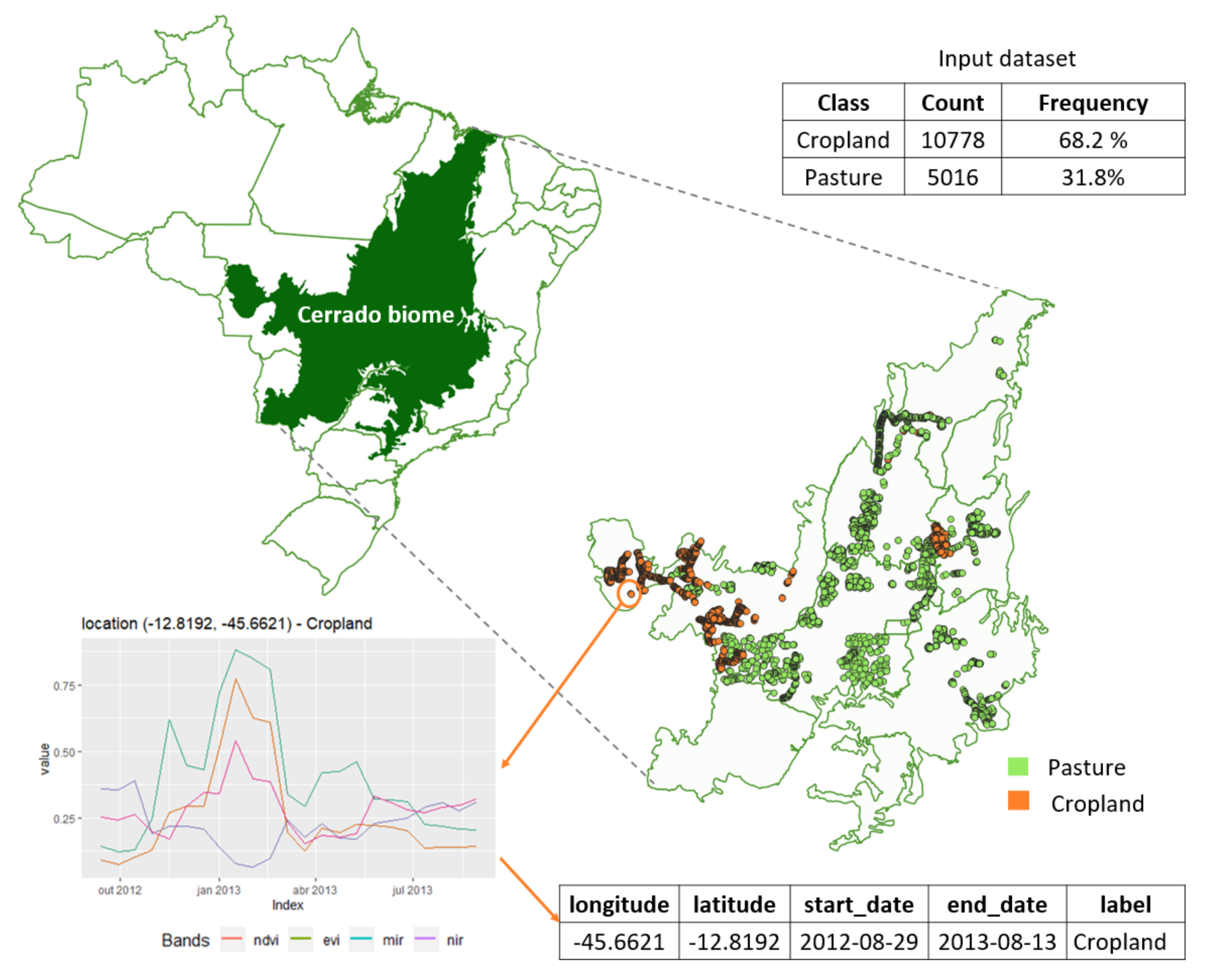
2.1. Data
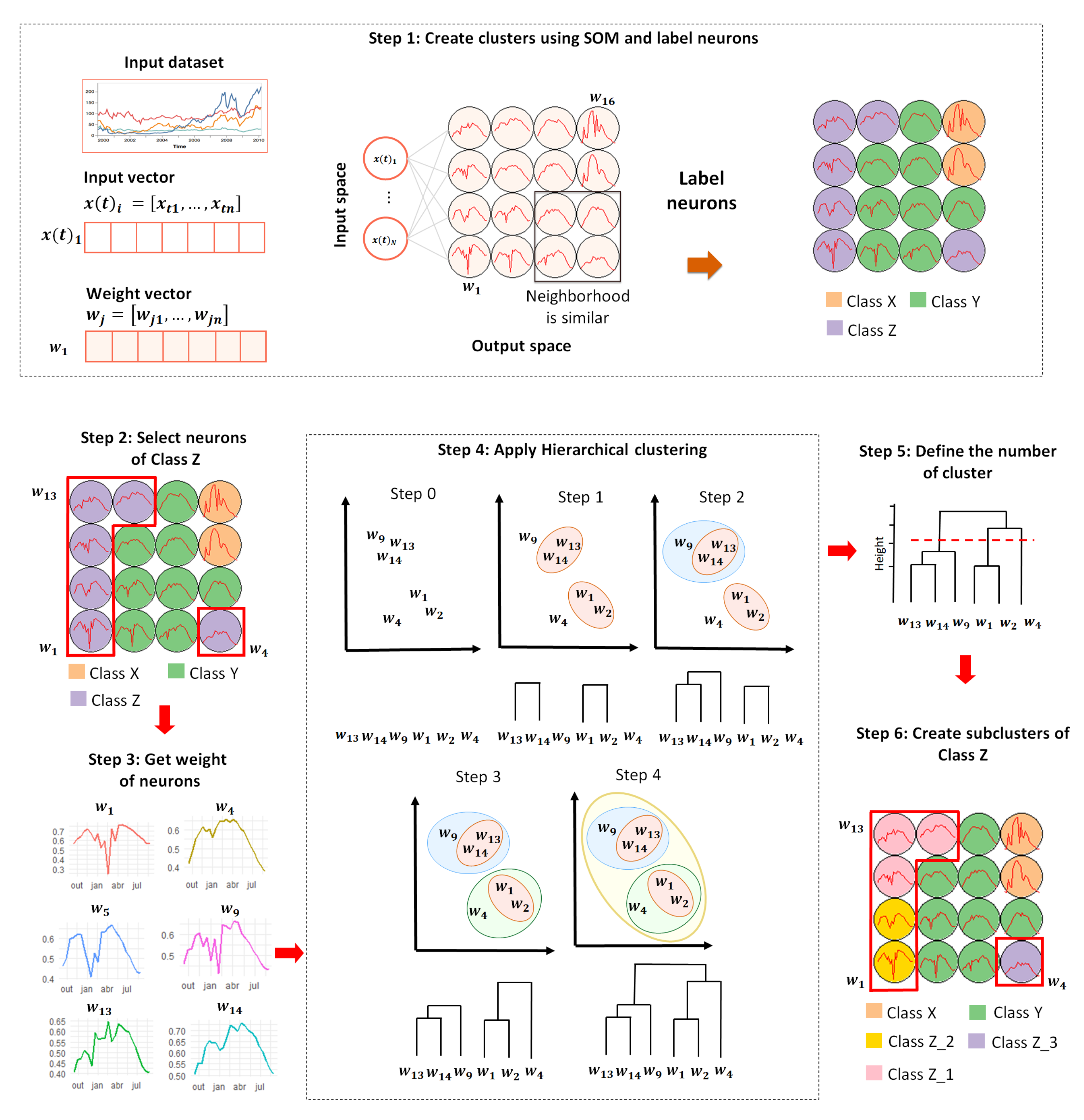
2.2. Overview
2.3. Self-Organizing Map
2.4. Hierarchical Clustering
2.5. Clustering Output
3. Results
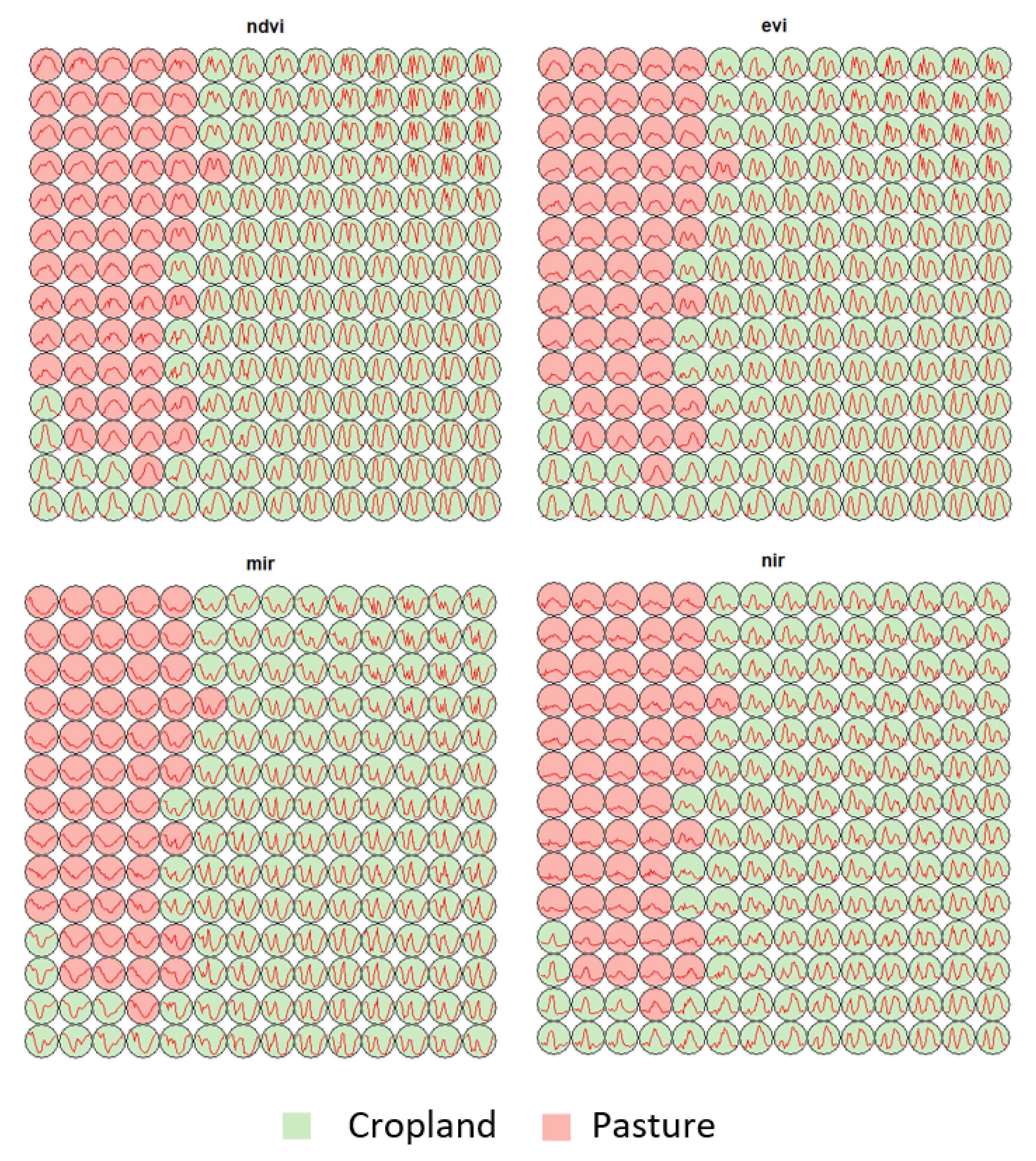
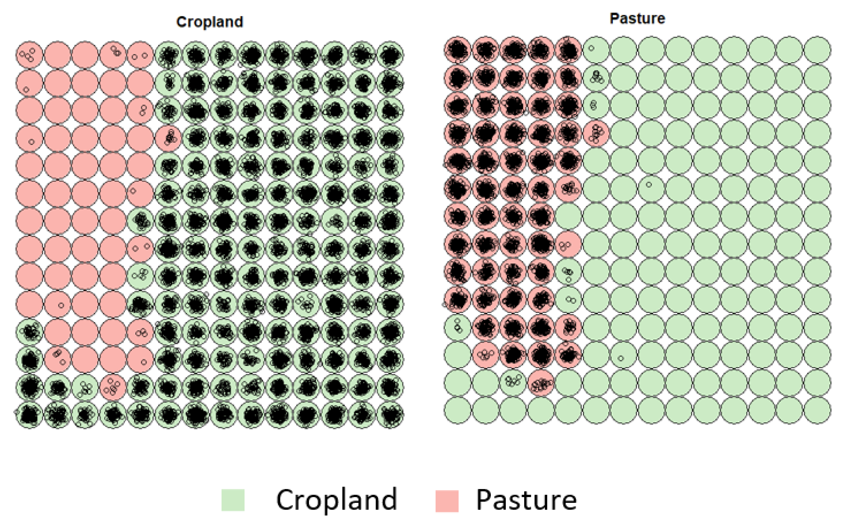
3.1. Creating Clusters Using SOM
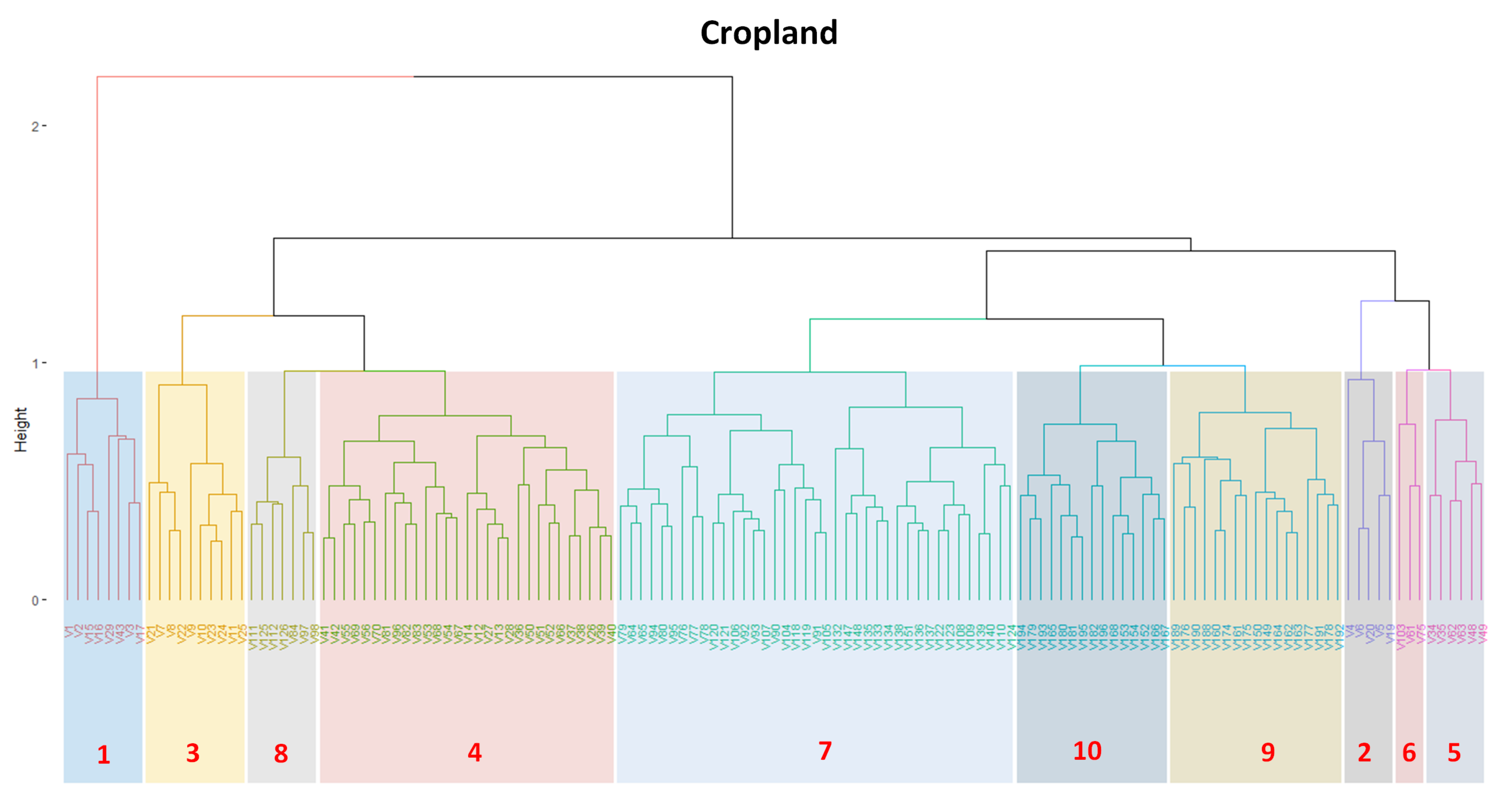
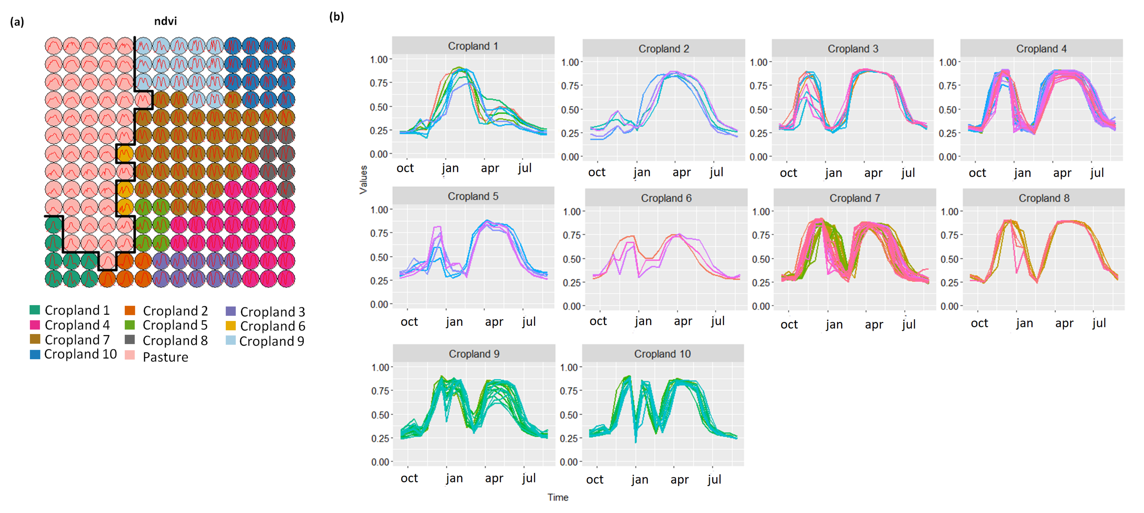
3.2. Revealing the Patterns of Cropland
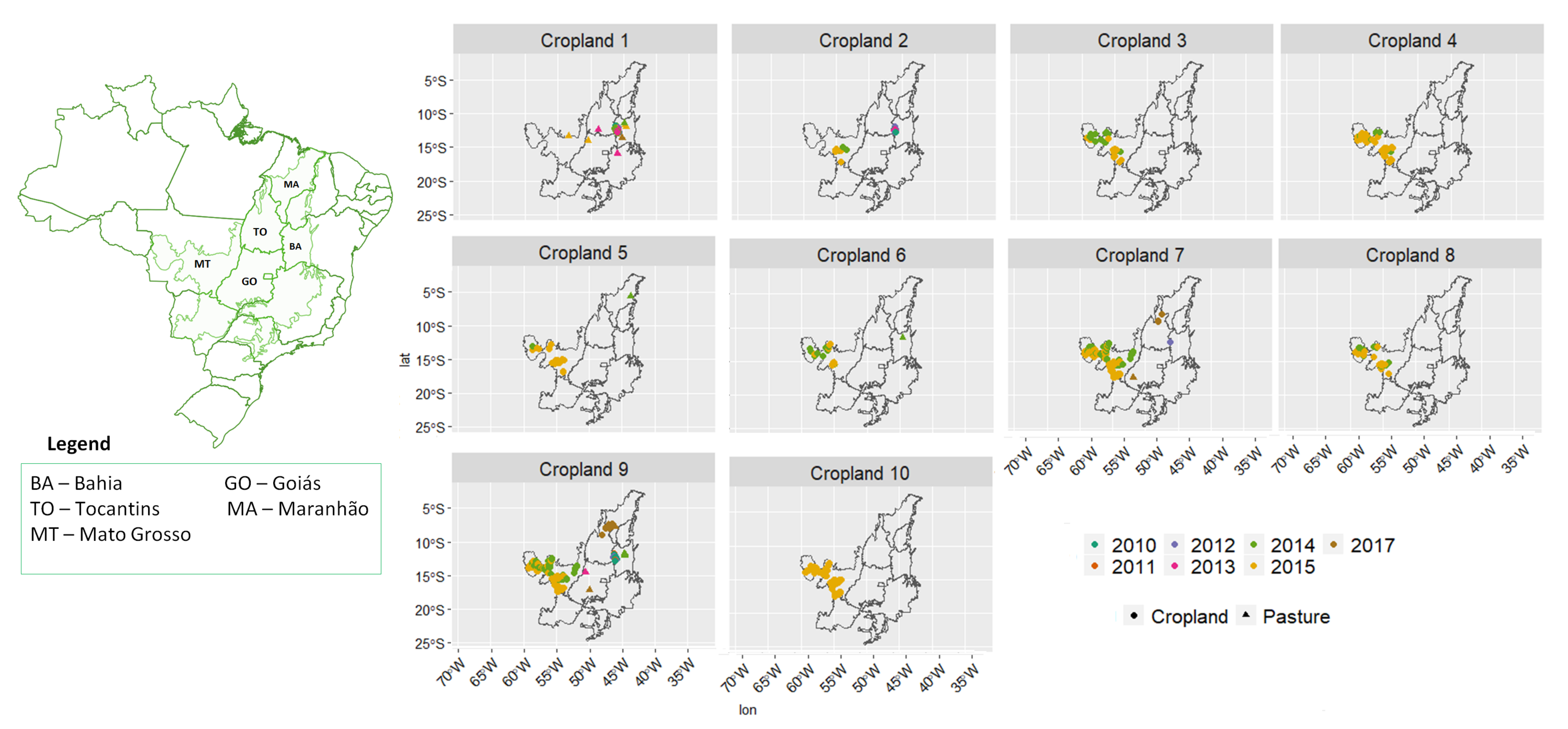
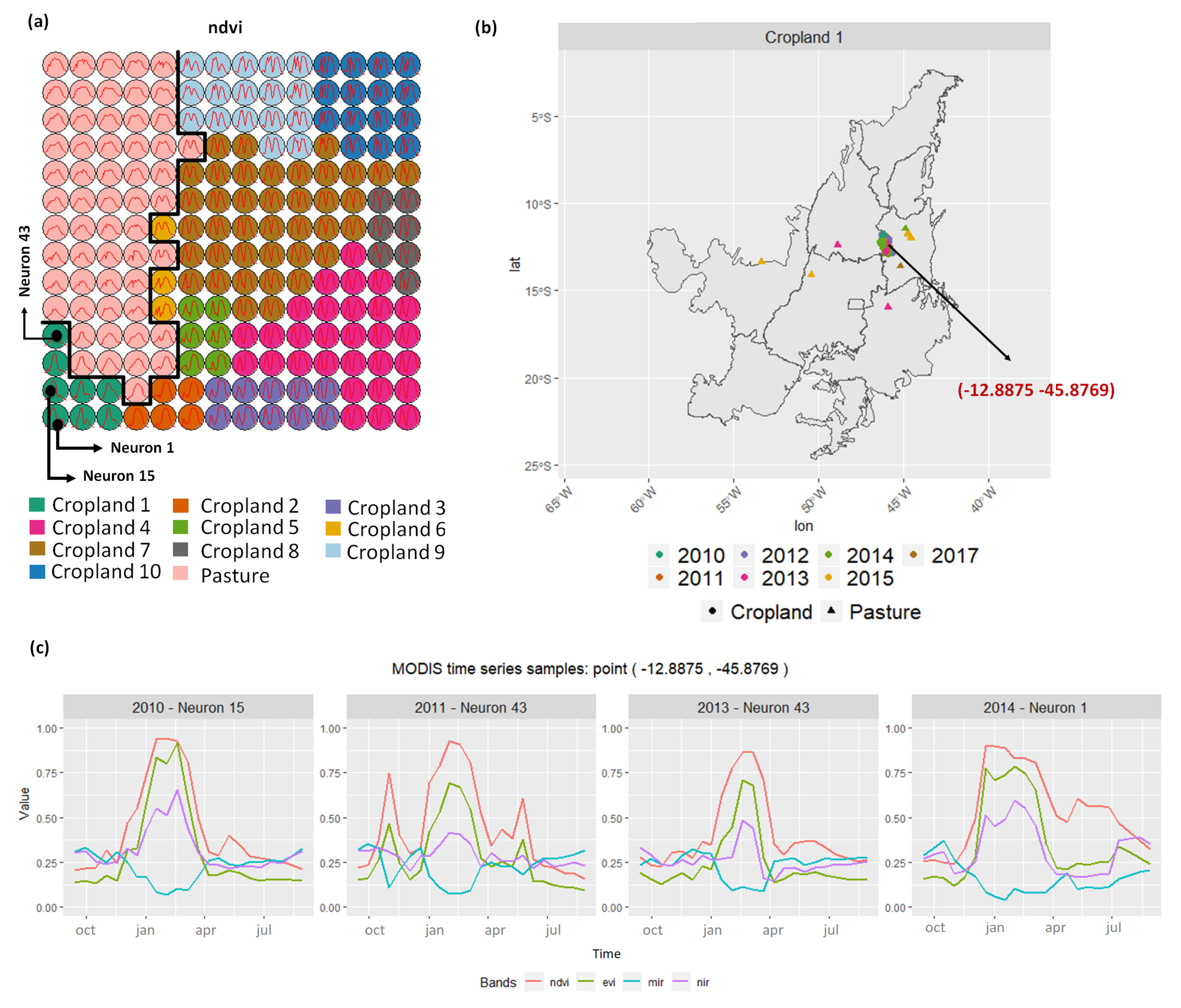
- Cropland 1 represents samples of soy–fallow. These samples are mapped only in the state of Bahia. This region is known due to the mostly single cropping regimes [58]. Some samples are spread over Goiás and Tocantins states; however, they are originally labeled as pasture.
- Cropland 2 represents samples of fallow–cotton. This type of crop is mapped in the states of Mato Grosso and Bahia. The patterns of this group are well defined.
- Croplands 3,4, and 8 represent samples of soy–cotton. In this study, this type of crop is mapped only in the state of Mato Grosso. Through the temporal patterns (Figure 7b), we can notice small variations, particularly during the first cycle (soy crop). This difference may be due to the soybean variety. The soybean varieties planted in Brazil can be of early, medium, and late maturity. The average cycle ranges from 99 to 128 days [59].
- Cropland 5 represents samples of millet–cotton. In this study, this type of crop is mapped only in the state of Mato Grosso.
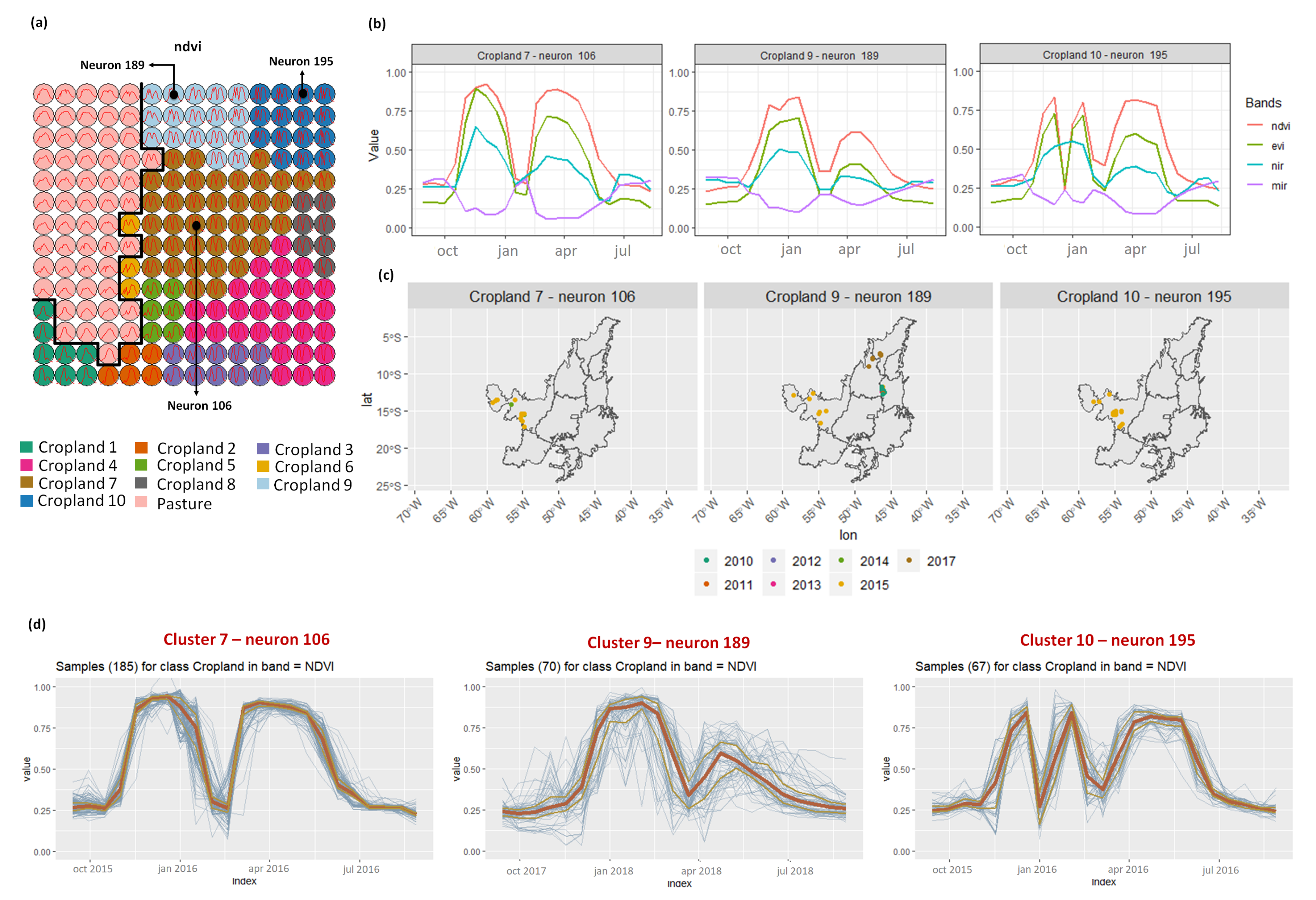
- Croplands 7, 9, and 10 represent samples of soy–corn. This type of crop is spread over the Cerrado biome. The variability of this class can be noticed through the temporal patterns extracted by SOM. It occurs due to the climatological and soil variations leading to differences in each area’s agricultural calendar.
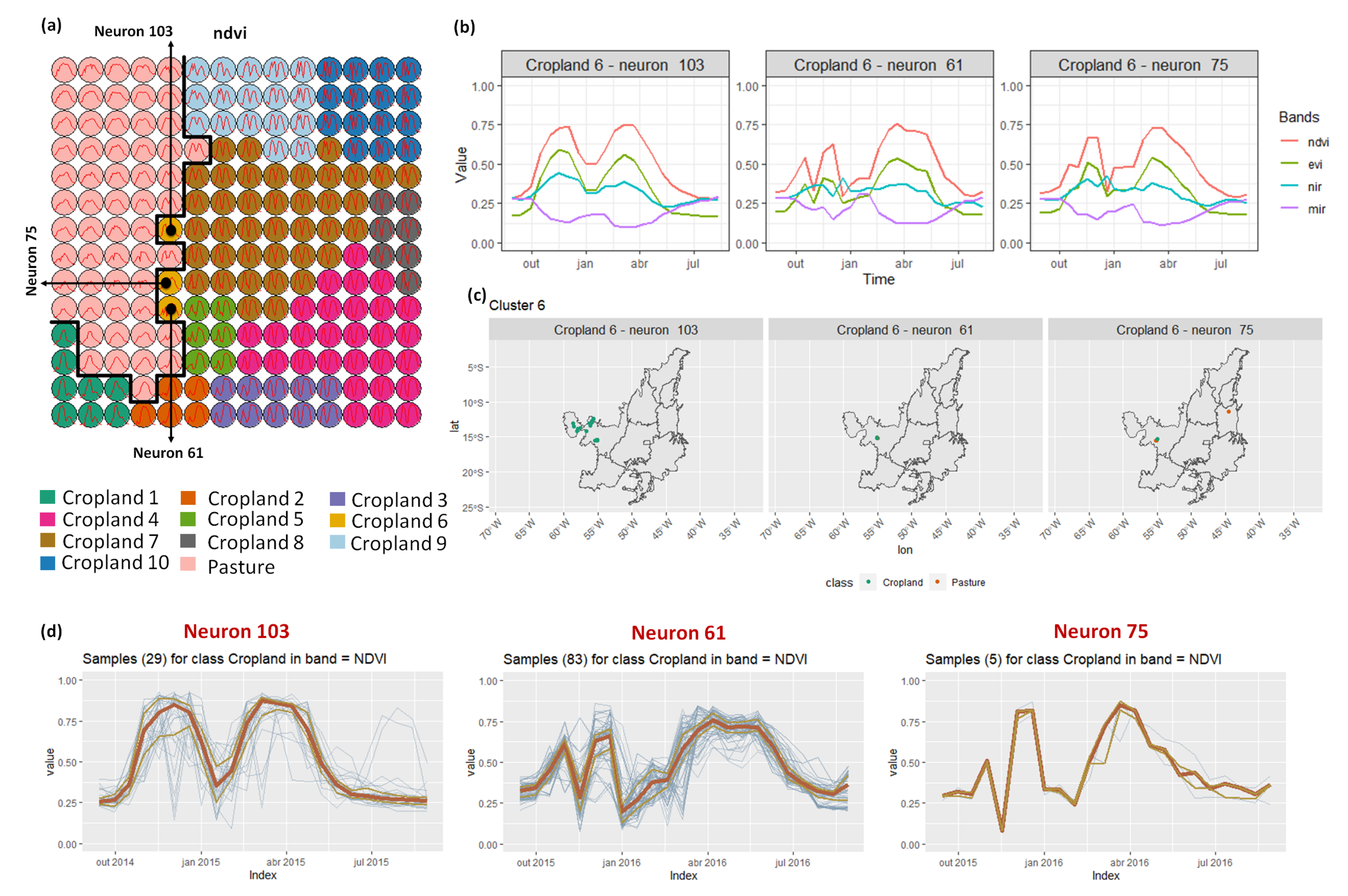
- Cropland 6 is not well defined. Notice in the SOM grid (Figure 7a) that most of the neighbors of Cropland 6 belong to other groups. The temporal signatures can be confounded between soy and millet during the first cycle due to noise, likely caused by clouds. It is necessary to look at these samples in more detail. In contrast, in the second cycle, we can notice patterns of cotton and corn. Additionally, this cluster contains samples initially labeled as pasture.
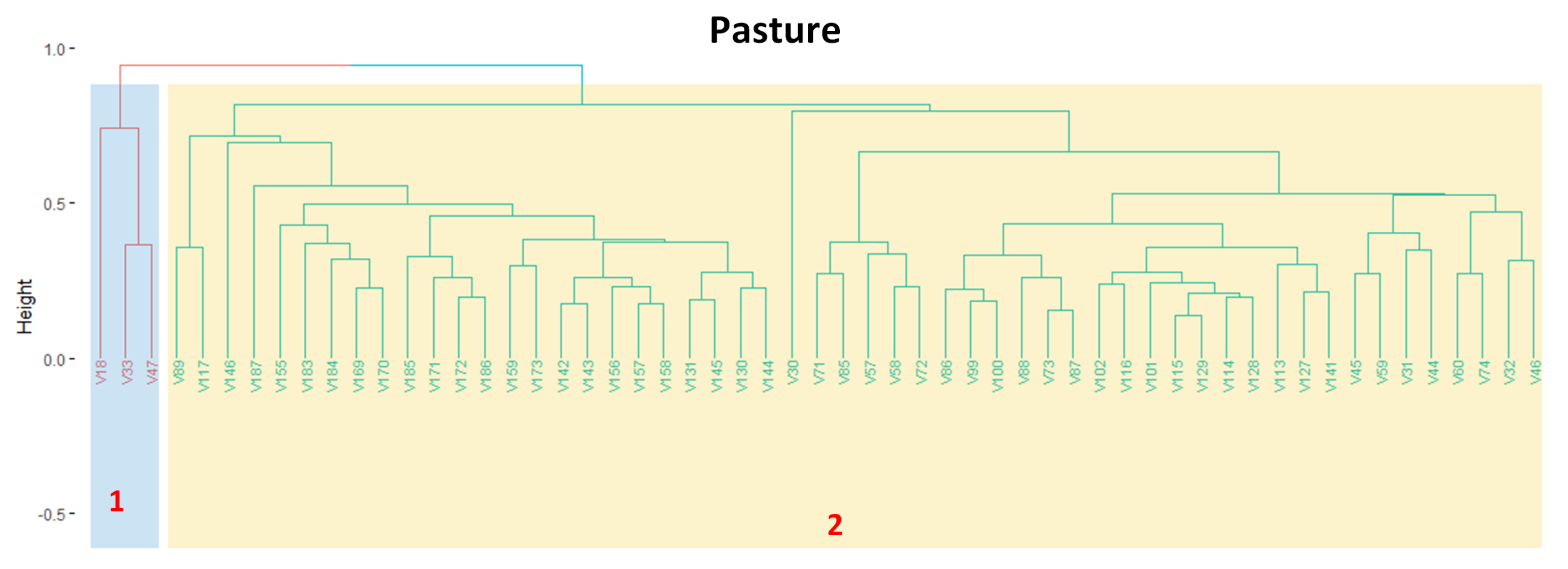
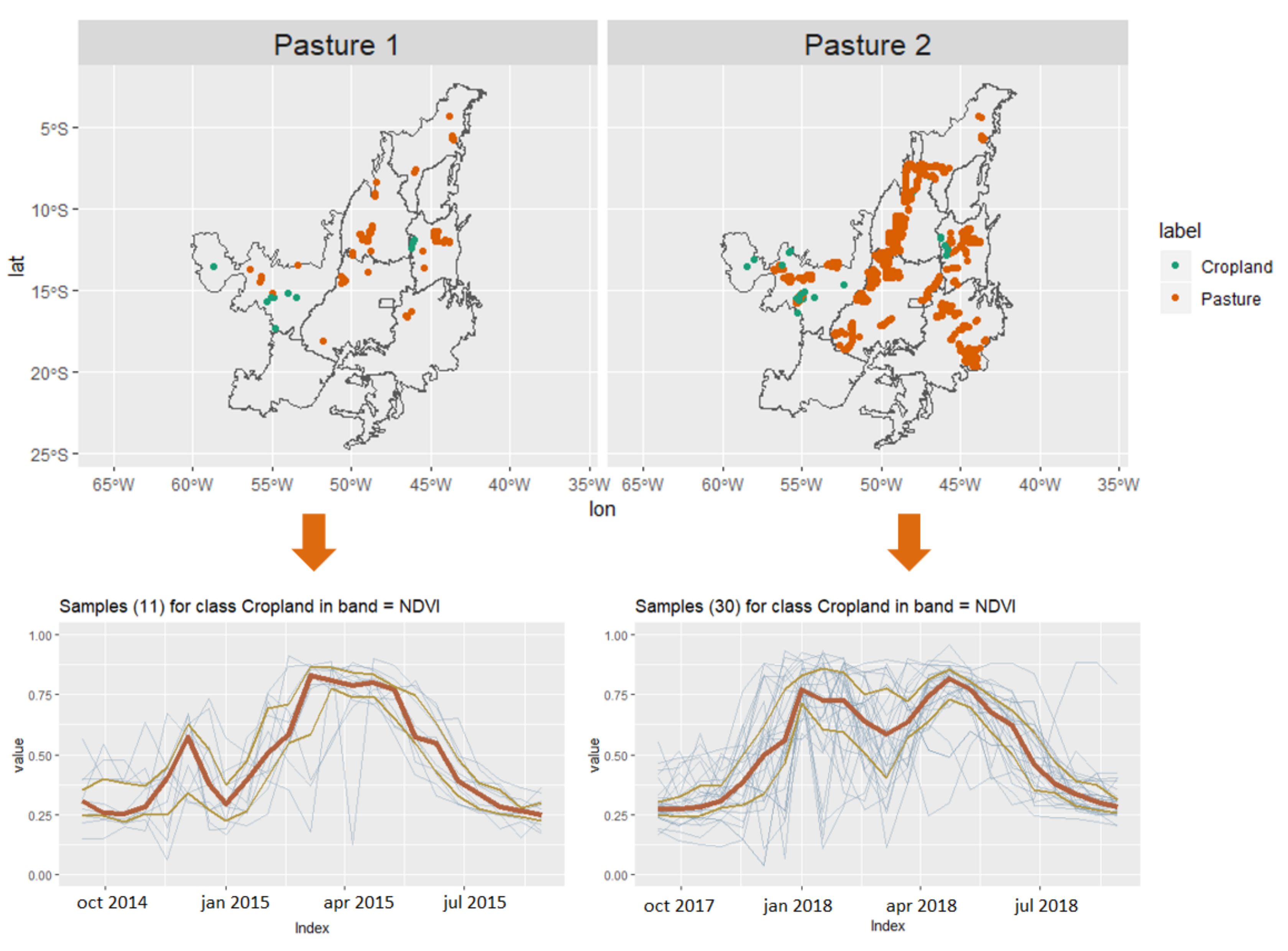
3.3. Revealing the Patterns of Pasture
3.4. Assessing the Performance of the Training Samples
4. Discussions
5. Conclusions
6. Data and Code Availability
Author Contributions
Funding
Institutional Review Board Statement
Informed Consent Statement
Data Availability Statement
Conflicts of Interest
References
- Gomez, C.; White, J.C.; Wulder, M.A. Optical Remotely Sensed Time Series Data for Land Cover Classification: A Review. ISPRS J. Photogramm. Remote. Sens. 2016, 116, 55–72. [Google Scholar] [CrossRef] [Green Version]
- Woodcock, C.E.; Loveland, T.R.; Herold, M.; Bauer, M.E. Transitioning from Change Detection to Monitoring with Remote Sensing: A Paradigm Shift. Remote Sens. Environ. 2020, 238, 111558. [Google Scholar] [CrossRef]
- Pasquarella, V.J.; Holden, C.E.; Kaufman, L.; Woodcock, C.E. From Imagery to Ecology: Leveraging Time Series of All Available LANDSAT Observations to Map and Monitor Ecosystem State and Dynamics. Remote Sens. Ecol. Conserv. 2016, 2, 152–170. [Google Scholar] [CrossRef]
- Millard, K.; Richardson, M. On the importance of training data sample selection in random forest image classification: A case study in peatland ecosystem mapping. Remote Sens. 2015, 7, 8489–8515. [Google Scholar] [CrossRef] [Green Version]
- Pelletier, C.; Valero, S.; Inglada, J.; Champion, N.; Marais Sicre, C.; Dedieu, G. Effect of Training Class Label Noise on Classification Performances for Land Cover Mapping with Satellite Image Time Series. Remote Sens. 2017, 9, 173. [Google Scholar] [CrossRef] [Green Version]
- Maxwell, A.E.; Warner, T.A.; Fang, F. Implementation of Machine-Learning Classification in Remote Sensing: An Applied Review. Int. J. Remote. Sens. 2018, 39, 2784–2817. [Google Scholar] [CrossRef] [Green Version]
- Pengra, B.W.; Stehman, S.V.; Horton, J.A.; Dockter, D.J.; Schroeder, T.A.; Yang, Z.; Cohen, W.B.; Healey, S.P.; Loveland, T.R. Quality control and assessment of interpreter consistency of annual land cover reference data in an operational national monitoring program. Remote Sens. Environ. 2020, 238, 111261. [Google Scholar] [CrossRef]
- Olofsson, P.; Foody, G.M.; Herold, M.; Stehman, S.V.; Woodcock, C.E.; Wulder, M.A. Good Practices for Estimating Area and Assessing Accuracy of Land Change. Remote Sens. Environ. 2014, 148, 42–57. [Google Scholar] [CrossRef]
- Elmes, A.; Alemohammad, H.; Avery, R.; Caylor, K.; Eastman, J.R.; Fishgold, L.; Friedl, M.A.; Jain, M.; Kohli, D.; Laso Bayas, J.C.; et al. Accounting for Training Data Error in Machine Learning Applied to Earth Observations. Remote Sens. 2020, 12, 1034. [Google Scholar] [CrossRef] [Green Version]
- Huang, H.; Wang, J.; Liu, C.; Liang, L.; Li, C.; Gong, P. The migration of training samples towards dynamic global land cover mapping. ISPRS J. Photogramm. Remote. Sens. 2020, 161, 27–36. [Google Scholar] [CrossRef]
- Viana, C.M.; Girão, I.; Rocha, J. Long-Term Satellite Image Time-Series for Land Use/Land Cover Change Detection Using Refined Open Source Data in a Rural Region. Remote Sens. 2019, 11, 1104. [Google Scholar] [CrossRef] [Green Version]
- Simoes, R.; Picoli, M.C.A.; Camara, G.; Maciel, A.; Santos, L.; Andrade, P.R.; Sánchez, A.; Ferreira, K.; Carvalho, A. Land Use and Cover Maps for Mato Grosso State in Brazil from 2001 to 2017. Sci. Data 2020, 7, 34. [Google Scholar] [CrossRef] [Green Version]
- Belgiu, M.; Bijker, W.; Csillik, O.; Stein, A. Phenology-based sample generation for supervised crop type classification. Int. J. Appl. Earth Obs. Geoinf. 2021, 95, 102264. [Google Scholar] [CrossRef]
- Demir, B.; Persello, C.; Bruzzone, L. Batch-mode active-learning methods for the interactive classification of remote sensing images. IEEE Trans. Geosci. Remote. Sens. 2010, 49, 1014–1031. [Google Scholar] [CrossRef] [Green Version]
- Tuia, D.; Volpi, M.; Copa, L.; Kanevski, M.; Munoz-Mari, J. A survey of active learning algorithms for supervised remote sensing image classification. IEEE J. Sel. Top. Signal Process. 2011, 5, 606–617. [Google Scholar] [CrossRef]
- Huang, X.; Weng, C.; Lu, Q.; Feng, T.; Zhang, L. Automatic labelling and selection of training samples for high-resolution remote sensing image classification over urban areas. Remote Sens. 2015, 7, 16024–16044. [Google Scholar] [CrossRef] [Green Version]
- Lu, Q.; Ma, Y.; Xia, G.S. Active learning for training sample selection in remote sensing image classification using spatial information. Remote Sens. Lett. 2017, 8, 1210–1219. [Google Scholar] [CrossRef]
- Solano-Correa, Y.T.; Bovolo, F.; Bruzzone, L. A Semi-Supervised Crop-Type Classification Based on Sentinel-2 NDVI Satellite Image Time Series And Phenological Parameters. In Proceedings of the 2019 IEEE International Geoscience and Remote Sensing Symposium (IGARSS 2019), Yokohama, Japan, 28 July–2 August 2019; pp. 457–460. [Google Scholar] [CrossRef]
- Radoux, J.; Lamarche, C.; Van Bogaert, E.; Bontemps, S.; Brockmann, C.; Defourny, P. Automated training sample extraction for global land cover mapping. Remote Sens. 2014, 6, 3965–3987. [Google Scholar] [CrossRef] [Green Version]
- Hostert, P.; Griffiths, P.; van-der-Linden, S.; Pflugmacher, D. Time Series Analyses in a New Era of Optical Satellite Data. In Remote Sensing Time Series: Revealing Land Surface Dynamics; Kuenzer, C., Dech, S., Wagner, W., Eds.; Springer International Publishing: Berlin/Heidelberg, Germany, 2015; pp. 25–41. [Google Scholar]
- Comber, A.; Wulder, M. Considering Spatiotemporal Processes in Big Data Analysis: Insights from Remote Sensing of Land Cover and Land Use. Trans. GIS 2019, 23, 879–891. [Google Scholar] [CrossRef]
- Alencar, A.; Shimbo, J.Z.; Lenti, F.; Balzani Marques, C.; Zimbres, B.; Rosa, M.; Arruda, V.; Castro, I.; Fernandes Márcico Ribeiro, J.P.; Varela, V.; et al. Mapping Three Decades of Changes in the Brazilian Savanna Native Vegetation Using Landsat Data Processed in the Google Earth Engine Platform. Remote Sens. 2020, 12, 924. [Google Scholar] [CrossRef] [Green Version]
- Meroni, M.; d’Andrimont, R.; Vrieling, A.; Fasbender, D.; Lemoine, G.; Rembold, F.; Seguini, L.; Verhegghen, A. Comparing land surface phenology of major European crops as derived from SAR and multispectral data of Sentinel-1 and -2. Remote Sens. Environ. 2021, 253, 112232. [Google Scholar] [CrossRef] [PubMed]
- Liao, T.W. Clustering of Time Series Data: A Survey. Pattern Recognit. 2005, 38, 1857–1874. [Google Scholar] [CrossRef]
- Aghabozorgi, S.; Shirkhorshidi, A.S.; Wah, T.Y. Time-Series Clustering: A Decade Review. Inf. Syst. 2015, 53, 16–38. [Google Scholar] [CrossRef]
- Paparrizos, J.; Gravano, L. k-shape: Efficient and accurate clustering of time series. In Proceedings of the 2015 ACM SIGMOD International Conference on Management of Data, Melbourne, Australia, 31 May – 4 June 2015; pp. 1855–1870. [Google Scholar]
- Birant, D.; Kut, A. ST-DBSCAN: An algorithm for clustering spatial–temporal data. Data Knowl. Eng. 2007, 60, 208–221. [Google Scholar] [CrossRef]
- Andrienko, G.; Andrienko, N.; Bremm, S.; Schreck, T.; Von Landesberger, T.; Bak, P.; Keim, D. Space-in-Time and Time-in-Space Self-Organizing Maps for Exploring Spatiotemporal Patterns. Comput. Graph. Forum 2010, 29, 913–922. [Google Scholar] [CrossRef]
- Augustijn, E.W.; Zurita-Milla, R. Self-Organizing Maps as an Approach to Exploring Spatiotemporal Diffusion Patterns. Int. J. Health Geogr. 2013, 12, 60. [Google Scholar] [CrossRef] [PubMed] [Green Version]
- Liu, H.; Zhan, Q.; Yang, C.; Wang, J. Characterizing the spatio-temporal pattern of land surface temperature through time series clustering: Based on the latent pattern and morphology. Remote Sens. 2018, 10, 654. [Google Scholar] [CrossRef] [Green Version]
- Qi, J.; Liu, H.; Liu, X.; Zhang, Y. Spatiotemporal evolution analysis of time-series land use change using self-organizing map to examine the zoning and scale effects. Comput. Environ. Urban Syst. 2019, 76, 11–23. [Google Scholar] [CrossRef]
- Xiong, J.; Thenkabail, P.S.; Gumma, M.K.; Teluguntla, P.; Poehnelt, J.; Congalton, R.G.; Yadav, K.; Thau, D. Automated cropland mapping of continental Africa using Google Earth Engine cloud computing. ISPRS J. Photogramm. Remote. Sens. 2017, 126, 225–244. [Google Scholar] [CrossRef] [Green Version]
- Wang, S.; Azzari, G.; Lobell, D.B. Crop type mapping without field-level labels: Random forest transfer and unsupervised clustering techniques. Remote Sens. Environ. 2019, 222, 303–317. [Google Scholar] [CrossRef]
- Hallac, D.; Vare, S.; Boyd, S.; Leskovec, J. Toeplitz inverse covariance-based clustering of multivariate time series data. In Proceedings of the 23rd ACM SIGKDD International Conference on Knowledge Discovery and Data Mining, Halifax, NS, Canada, 13–17 August 2017; pp. 215–223. [Google Scholar]
- Kohonen, T. The Self-Organizing Map. Proc. IEEE 1990, 78, 1464–1480. [Google Scholar] [CrossRef]
- Leonard Kaufman, P.J.R. Finding Groups in Data: An Introduction to Cluster Analysis, 9th ed.; Wiley-Interscience: Hoboken, NJ, USA, 1990. [Google Scholar]
- Everitt, B.S.; Landau, S.; Leese, M.; Stahl, D. Cluster Analysis, 5th ed.; Wiley Series in Probability and Statistics; Wiley: Hoboken, NJ, USA, 2011. [Google Scholar]
- Zurita-Milla, R.; Van Gijsel, J.; Hamm, N.A.; Augustijn, P.; Vrieling, A. Exploring spatiotemporal phenological patterns and trajectories using self-organizing maps. IEEE Trans. Geosci. Remote. Sens. 2012, 51, 1914–1921. [Google Scholar] [CrossRef]
- Chen, I.T.; Chang, L.C.; Chang, F.J. Exploring the spatio-temporal interrelation between groundwater and surface water by using the self-organizing maps. J. Hydrol. 2018, 556, 131–142. [Google Scholar] [CrossRef]
- Guo, D.; Chen, J.; MacEachren, A.M.; Liao, K. A visualization system for space-time and multivariate patterns (vis-stamp). IEEE Trans. Vis. Comput. Graph. 2006, 12, 1461–1474. [Google Scholar] [PubMed] [Green Version]
- Astel, A.; Tsakovski, S.; Barbieri, P.; Simeonov, V. Comparison of self-organizing maps classification approach with cluster and principal components analysis for large environmental data sets. Water Res. 2007, 41, 4566–4578. [Google Scholar] [CrossRef] [PubMed]
- Liu, Y.; Weisberg, R.H. A review of self-organizing map applications in meteorology and oceanography. In Self-Organizing Maps: Applications and Novel Algorithm Design; InTech: Rijeka, Croatia, 2011; pp. 253–272. [Google Scholar]
- Dickie, A.; Magno, I.; Giampietro, J.; Dolginow, A. Challenges and Opportunities for Conservation, Agricultural Production, and Social Inclusion in the Cerrado Biome; Technical Report; CEA Consulting: San Francisco, CA, USA, 2016. [Google Scholar]
- Soterroni, A.C.; Ramos, F.M.; Mosnier, A.; Fargione, J.; Andrade, P.R.; Baumgarten, L.; Pirker, J.; Obersteiner, M.; Kraxner, F.; Camara, G.; et al. Expanding the Soy Moratorium to Brazil’s Cerrado. Sci. Adv. 2019, 5, eaav7336. [Google Scholar] [CrossRef] [Green Version]
- Klink, C.; Machado, R. Conservation of the Brazilian Cerrado. Conserv. Biol. 2005, 19, 707–713. [Google Scholar] [CrossRef]
- Ansari, M.Y.; Ahmad, A.; Khan, S.S.; Bhushan, G.; Mainuddin. Spatiotemporal clustering: A review. Artif. Intell. Rev. 2019, 53, 2381–2423. [Google Scholar] [CrossRef]
- Wu, X.; Cheng, C.; Zurita-Milla, R.; Song, C. An overview of clustering methods for geo-referenced time series: From one-way clustering to co- and tri-clustering. Int. J. Geogr. Inf. Sci. 2020, 34, 1822–1848. [Google Scholar] [CrossRef]
- Johnson, S.C. Hierarchical clustering schemes. Psychometrika 1967, 32, 241–254. [Google Scholar] [CrossRef]
- Natita, W.; Wiboonsak, W.; Dusadee, S. Appropriate Learning Rate and Neighborhood Function of Self-Organizing Map (SOM) for Specific Humidity Pattern Classification over Southern Thailand. Int. J. Model. Optim. 2016, 6. [Google Scholar] [CrossRef] [Green Version]
- Kohonen, T. Essentials of the Self-Organizing Map. Neural Netw. 2013, 37, 52–65. [Google Scholar] [CrossRef]
- Kohonen, T.; Kaski, S.; Lagus, K.; Salojarvi, J.; Honkela, J.; Paatero, V.; Saarela, A. Self organization of a massive document collection. IEEE Trans. Neural Netw. 2000, 11, 574–585. [Google Scholar] [CrossRef] [Green Version]
- Hubert, L.J.; Levin, J.R. A general statistical framework for assessing categorical clustering in free recall. Psychol. Bull. 1976, 83, 1072. [Google Scholar] [CrossRef]
- Arlot, S.; Celisse, A. A survey of cross-validation procedures for model selection. Stat. Surv. 2010, 4, 40–79. [Google Scholar] [CrossRef]
- Bengio, Y.; Grandvalet, Y. No Unbiased Estimator of the Variance of K-Fold Cross-Validation. J. Mach. Learn. Res. 2004, 5, 1089–1105. [Google Scholar]
- Belgiu, M.; Dragut, L. Random Forest in Remote Sensing: A Review of Applications and Future Directions. ISPRS J. Photogramm. Remote. Sens. 2016, 114, 24–31. [Google Scholar] [CrossRef]
- Santos, L.; Ferreira, K.; Picoli, M.; Camara, G. Self-Organizing Maps in Earth Observation Data Cubes Analysis. In Advances in Self-Organizing Maps, Learning Vector Quantization, Clustering and Data Visualization; Vellido, A., Gibert, K., Angulo, C., Martin, J., Eds.; Springer International Publishing: Berlin/Heidelberg, Germany, 2019; pp. 70–79. [Google Scholar]
- Vesanto, J.; Alhoniemi, E. Clustering of the self-organizing map. IEEE Trans. Neural Networks 2000, 11, 586–600. [Google Scholar] [CrossRef] [PubMed]
- Sanches, I.D.; Feitosa, R.Q.; Achanccaray, P.; Montibeller, B.; Luiz, A.J.B.; Soares, M.D.; Prudente, V.H.R.; Vieira, D.C.; Maurano, L.E.P. Lem Benchmark Database for Tropical Agricultural Remote Sensing Application. ISPRS Int. Arch. Photogramm. Remote. Sens. Spat. Inf. Sci. 2018, XLII-1, 387–392. [Google Scholar] [CrossRef] [Green Version]
- Zito, R.K.; Filho, O.L.d.M.; Pereira, M.J.Z.; Meyer, M.C.; Hirose, E.; Nicoli, C.M.L.; Costa, S.V.d.; de Neto, C.D.M.; Nunes, J., Jr.; Vieira, N.E.; et al. Cultivares de soja: Macrorregiões 3, 4 e 5 Goiás e Região Central do Brasil. 2018. Available online: https://www.embrapa.br/en/busca-de-publicacoes/-/publicacao/1067791/cultivares-de-soja-macrorregioes-3-4-e-5-goias-e-regiao-central-do-brasil (accessed on 15 July 2020).
- Abrahão, G.M.; Costa, M.H. Evolution of rain and photoperiod limitations on the soybean growing season in Brazil: The rise (and possible fall) of double-cropping systems. Agric. For. Meteorol. 2018, 256–257, 32–45. [Google Scholar] [CrossRef]
- Alonso, M.P.; Moraes, E.; Pereira, D.H.; Pina, D.S.; Mombach, M.A.; Hoffmann, A.; de Moura Gimenez, B.; Sanson, R.M.M. Pearl millet grain for beef cattle in crop-livestock integration system: Intake and digestibility. Semin. Cienc. Agrar. 2017, 38, 1471–1482. [Google Scholar] [CrossRef] [Green Version]
- Embrapa. O Cerrado. 2020. Available online: http://www.cpac.embrapa.br/unidade/ocerrado (accessed on 14 September 2020).
- Jensen, J.R. Remote Sensing of the Environment: An Earth Resource Perspective, 2nd ed.; Pearson: London, UK, 2009. [Google Scholar]
- Picoli, M.; Camara, G.; Sanches, I.; Simoes, R.; Carvalho, A.; Maciel, A.; Coutinho, A.; Esquerdo, J.; Antunes, J.; Begotti, R.A.; et al. Big Earth Observation Time Series Analysis for Monitoring Brazilian Agriculture. ISPRS J. Photogramm. Remote. Sens. 2018, 145, 328–339. [Google Scholar] [CrossRef]
- Ferreira, K.; Santos, L.; Picoli, M. Evaluating Distance Measures for Image Time Series Clustering in Land Use and Cover Monitoring. In MACLEAN 2019 MAChine Learning for EArth ObservatioN Workshop; CEUR-WS: Würzburg, Germany, 2019. [Google Scholar]
- Ferreira, K.R.; Queiroz, G.R.; Vinhas, L.; Marujo, R.F.B.; Simoes, R.E.O.; Picoli, M.C.A.; Camara, G.; Cartaxo, R.; Gomes, V.C.F.; Santos, L.A.; et al. Earth Observation Data Cubes for Brazil: Requirements, Methodology and Products. Remote Sens. 2020, 12, 4033. [Google Scholar] [CrossRef]


| Cluster | Count | Frequency | Class |
|---|---|---|---|
| 1. Cropland_Pasture | 41 | 0.26% | Cropland |
| 2. Cropland_1 | 563 | 3.5% | Soy–Fallow |
| 3. Cropland_2 | 348 | 2.2 % | Fallow–Cotton |
| 4. Cropland_3_4_6_8 | 3866 | 24.5 % | Soy–Cotton |
| 5. Cropland_5 | 429 | 2.8 % | Millet–Cotton |
| 6. Cropland_6_7_9_10 | 5331 | 34.5% | Soy–Corn |
| 7. Pasture_1 | 90 | 0.58% | Pasture_1 |
| 8. Pasture_2 | 4926 | 31.2% | Pasture_2 |
| 1 | 2 | 3 | 4 | 5 | 6 | 7 | 8 | UA | |
|---|---|---|---|---|---|---|---|---|---|
| 1. Cropland | 5 | 0 | 0 | 0 | 0 | 0 | 0 | 0 | 100% |
| 2. Soy–Corn | 23 | 5372 | 33 | 63 | 1 | 7 | 6 | 1 | 97% |
| 3. Soy–Cotton | 0 | 50 | 3912 | 27 | 11 | 0 | 1 | 1 | 97% |
| 4. Millet–Cotton | 0 | 1 | 4 | 339 | 0 | 0 | 1 | 0 | 98% |
| 5. Fallow–Cotton | 6 | 1 | 2 | 0 | 334 | 0 | 0 | 0 | 97% |
| 6. Soy–Fallow | 2 | 13 | 0 | 0 | 1 | 552 | 0 | 0 | 97% |
| 7. Pasture_2 | 5 | 6 | 3 | 0 | 1 | 4 | 4978 | 61 | 98% |
| 8. Pasture_1 | 0 | 0 | 0 | 0 | 0 | 0 | 0 | 27 | 100% |
| PA | 12% | 98% | 98% | 79% | 95% | 98% | 99% | 30% | 98% |
| 1 | 2 | 3 | 4 | 5 | 6 | 7 | UA | |
|---|---|---|---|---|---|---|---|---|
| 1. Soy–Corn | 5365 | 31 | 68 | 1 | 7 | 6 | 1 | 97% |
| 2. Soy–Cotton | 58 | 3913 | 28 | 9 | 0 | 1 | 0 | 97% |
| 3.Millet–Cotton | 1 | 3 | 333 | 0 | 0 | 1 | 0 | 98% |
| 4. Fallow–Cotton | 1 | 3 | 0 | 336 | 0 | 0 | 0 | 98% |
| 5. Soy–Fallow | 13 | 0 | 0 | 1 | 551 | 0 | 0 | 97% |
| 6. Pasture_2 | 5 | 4 | 0 | 1 | 5 | 4918 | 61 | 98% |
| 7. Pasture_1 | 0 | 0 | 0 | 0 | 0 | 0 | 28 | 100% |
| PA | 98% | 98% | 77% | 96% | 97% | 99% | 31% | 97% |
| Pasture | Cropland | UA | |
|---|---|---|---|
| Pasture | 4980 | 17 | 99% |
| Cropland | 36 | 10761 | 99% |
| PA | 99% | 99% | 99% |
Publisher’s Note: MDPI stays neutral with regard to jurisdictional claims in published maps and institutional affiliations. |
© 2021 by the authors. Licensee MDPI, Basel, Switzerland. This article is an open access article distributed under the terms and conditions of the Creative Commons Attribution (CC BY) license (http://creativecommons.org/licenses/by/4.0/).
Share and Cite
Santos, L.A.; Ferreira, K.; Picoli, M.; Camara, G.; Zurita-Milla, R.; Augustijn, E.-W. Identifying Spatiotemporal Patterns in Land Use and Cover Samples from Satellite Image Time Series. Remote Sens. 2021, 13, 974. https://doi.org/10.3390/rs13050974
Santos LA, Ferreira K, Picoli M, Camara G, Zurita-Milla R, Augustijn E-W. Identifying Spatiotemporal Patterns in Land Use and Cover Samples from Satellite Image Time Series. Remote Sensing. 2021; 13(5):974. https://doi.org/10.3390/rs13050974
Chicago/Turabian StyleSantos, Lorena Alves, Karine Ferreira, Michelle Picoli, Gilberto Camara, Raul Zurita-Milla, and Ellen-Wien Augustijn. 2021. "Identifying Spatiotemporal Patterns in Land Use and Cover Samples from Satellite Image Time Series" Remote Sensing 13, no. 5: 974. https://doi.org/10.3390/rs13050974