Abstract
In the recent decades, development of agricultural and human settlements have severely affected wetlands on the China-side of the Amur River Basin (CARB). A long-term holistic view of spatio-temporal variations of the wetlands on the CARB is essential for supporting sustainable conservation of wetlands in this region. In this study, a training sample migration method along with Random Forest classifier were adopted to map wetland and other land covers from two key seasons image collections. The proposed classification method was applied to Landsat images, and a 30-m resolution dataset was obtained, which reflected the dynamic changes of historical wetland distribution on the CARB region from 1990 to 2010. As the accuracy assessments showed, land cover maps of the CARB had high accuracies. The classification results indicated that the wetland area decreased from 89,432 km2 to 75,061 km2 between 1990 and 2010, with a net loss of 16%, which was mainly converted to paddy field and dry farmland, and the changes were most obvious in Sanjiang Plain and Songnen Plain. This suggests that agricultural activities are the main cause of wetland loss. The results can provide reliable information for the research on wetland management and sustainable development of the society and economy in the CARB.
1. Introduction
Wetlands, known as the kidneys of the Earth, cover approximately 6% of the terrestrial area and provide numerous ecosystem services, such as maintaining water balance, sequestrating carbon, regulating climate, and providing habitat [1,2]. However, since the eighteenth century, up to 87% of wetlands have been lost globally, and severe degradation has happened in Asia as well as many high- and mid-latitude regions [3,4]. Tracking historical changes of wetlands is fundamental for wetland conservation and restoration, and serves as a key role in related decision-making processes.
The Amur River Basin, spans Russia, China, and Mongolia, and is one of the world’s top ten largest river basins [5]. The wetlands in it provide abundant breeding habitats for migratory waterfowl on the East Asia–Australasia Flyway (EAAF) [4]. However, compared with Europe and North America at the same latitudes, this basin has a unique landscape pattern [6] but less focus. Nowadays, population in the China side account more than 93% of the total population in the whole Basin. Since the early 1950s, human settlement and agricultural development in the China side of the Amur River Basin (CARB) have severely affected local natural wetlands [7,8]. Thus, the ecosystem services of wetlands on the CARB have been largely degraded. A holistic view of spatio-temporal variations of the wetlands on the CARB is essential for evaluating ecosystem services and supporting sustainable conservation of wetlands in this region.
Remote sensing, which could provide historical and current patterns of natural resources, has long been used to track wetland changes [9,10,11]. Among varieties of remote sensing data, Landsat-5, which afforded the first image obtained in the year of 1984, was widely applied to historical wetland mapping [12]. To date, numerous classification methods were employed to map wetland changes [13,14,15]. Traditionally, accurate mapping of the complex wetland landscape depended on manually interpreting, empirical thresholds, or post-processing. However, such approaches are usually laborious and costly in large-scale applications. In recent years, to address the limitations brought by traditional methods, machine learning algorithms (MLAs) have been adopted in mapping wetlands. Due to the robustness and accuracy, random forest (RF) classifier is the widest used of the MLAs [16,17,18], which has also been adopted to wetland mapping processes [19].
Lack of suitable training samples is the greatest challenge hindering the progress of MLAs-based wetland mapping across broad scales [20]. In general, the accuracy of supervised classification is significantly influenced by the quality of training samples. In many classification processes, errors could be caused by inappropriate or unrepresentative training samples, no matter what algorithms were being used [21,22,23]. However, for large scale applications, problems associated with the sample collection, such as cost and practicality, have been the limiting factors for acquiring consistent and high-quality samples. Moreover, due to the unavailability of historical field samples, the historical imagery can hardly be classified by the MLAs. Recently, Huang et al. [20] developed a training sample migration method which could identify the changing state of training sample pixels and form historical training samples automatically. This sample migration method provides opportunities to map historical land cover based on MLAs. However, more attempts need to be explored on broader scales.
In recent years, individual geoscientists who are interested in geospatial analysis have benefited from the Google Earth Engine (GEE) platform [24,25]. This cloud-based platform has introduced possibilities for automatic training sample migration and supports RF-based wetland mapping. Thus, the aim of this study was to track historical changes of wetlands on the CARB based on Landsat images. To achieve this goal, we sought to (1) operate an automatic training sample migration method which could form historical training sample collections of the CARB for the time periods of 2010, 2000, and 1990; (2) based on the historical training sample collections, we applied RF classifier to map wetlands and other land cover; and (3) analyzed dynamics and conversions of wetland on the CARB. The methods and discussion will contribute to remote sensing and management of the wetlands around the world.
2. Materials and Methods
2.1. Study Area
The Amur River Basin ranks the tenth largest watershed in the world. The area of the CARB is 890,308 km2, including parts of the Jilin and Inner Mongolia provinces and the whole Heilongjiang province (41°45′N to 53°33′N, 115°13′E to 135°05′E, Figure 1). The Greater Khingan, Lesser Khingan and Changbai mountains are located in the western, northern, and eastern side, respectively. While the Songnen and the Sanjiang Plain are situated in the interior and northeastern, respectively. The Ussuri and Songhua rivers are major tributaries of the CARB [26,27].
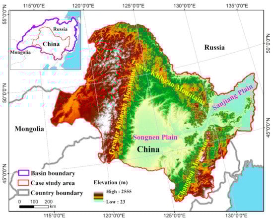
Figure 1.
Spatial location and elevation of the China side of the Amur River Basin (CARB).
2.2. Land Cover Classification System
Referring to our primary research objectives, and considering the results of our field surveys, land cover classification system of the CARB is defined in Table 1. Wetlands, in this study, were referred to as vegetated wetland and included four types, (i.e., swamp, marsh, bog, and fen).

Table 1.
Land cover classification system for the CARB.
2.3. Basic Idea
In this study, there were four steps to map the wetland and surrounding land covers. The flow chart is illustrated in Figure 2. First of all, establishing Landsat Thematic Mapper (TM) image collection (Section 2.4); and then, the migration of training samples (Section 2.5); thirdly, using RF classifier and training samples to map wetland and other land covers in the three historical time periods (Section 2.6); and lastly, assessing classification accuracies using independent ground reference samples (Section 2.7).
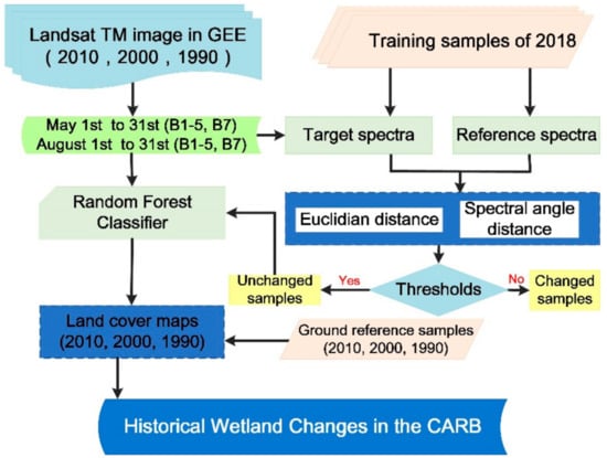
Figure 2.
Workflow of land cover mapping of the CARB.
2.4. Landsat-5 Data Collection in the GEE
Ideally, accurate training sample migration needs to be applied to consistent images acquired in the same phenological period and from the same sensor [28]. Thus, in this study, Landsat-5 Thematic Mapper (TM) which hold the Guinness World Record for the longest on-orbit time (from 1984 to 2012) were used to monitor historical wetlands on the CARB. In total, 78 tiles of Landsat images could cover the CARB completely. We selected cloud free Landsat images captured during two key phenological periods that could distinguish wetland and other land covers. These periods were from 1 May to 31 May and from 1 August to 31 August. In order to assure the quality of observations, images captured in the same key phenological periods of years adjacent to 1990, 2000, and 2010 were also selected. For each location, the images with the highest quality were used to migrate training samples and classify wetland and other land covers. Finally, the image collection contained 468 TM calibrated surface reflectance images in total.
2.5. Training Samples Collection and Migration
Ground surveys were conducted between June and September 2018. Ground reference data were also collected from historic field surveys between 2000 and 2010. Samples from a 1990 field survey were drawn from historical maps and documents with the assistance of local experts. Finally, we collected 7325, 9016, 18,315 and 24,422 reference samples for 1990, 2000, 2010 and 2018, respectively. Among these data, samples collected during 2018 were used to migrate to the training samples of the years 2010, 2000, and 1990, while other ground reference samples acquired for the years of 1990, 2000, and 2010 were used to validate classification accuracies. Spatial distributions of 2018′s ground reference samples were shown in Figure 3.
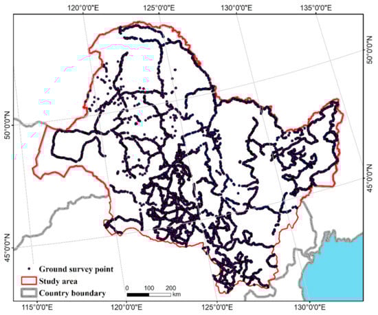
Figure 3.
Ground survey samples obtained in the year 2018.
Analyzing the spectral similarity and difference among different land covers is the first step for a classification task based on remote sensing. In this study, 200 ground survey samples for each land cover type were selected randomly. Then we overlaid these samples with the 2010 Landsat 5 images obtained in May and August 2010. Figure 4 shows the surface reflectance of typical land covers. It is as expected that the general shapes of the spectral curves were similar, especially in bands 1–3 which revealed a considerable overlap of both May and August. In the spectral region of band 4 (760–900 nm) in May, the reflectance of woodland was similar to dry farmland, while in band 4 of August, woodland was much lower than dry farmland. By comparison, the reflectance of wetland was obviously different to paddy field. These spectra can be considered as an important estimate to map different land covers on the CARB.
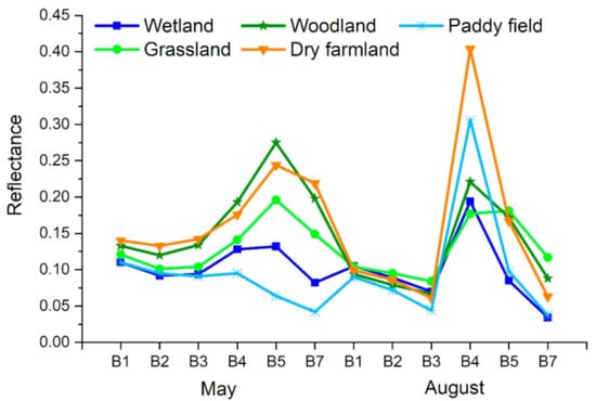
Figure 4.
Mean reflectance spectra of wetland and other land covers.
2.6. Training Samples Migration
To migrate training samples from a reference year to a target year, differences between the two spectra should be measured. In this study, euclidean distance (ED) and spectral angle distance (SAD) were chosen to realize this goal. The results show that these two indices are the best order of magnitude and similarity for the detection of bitemporal changes [12,20]. SAD can measure the angle between two vectors by the direction of changes. It is insensitive to illumination variation and shadow, and can stress the spectral shape characteristics of the target [29,30].
where θ represents the spectral angle. Xi is the reference spectra of time t1, Yi is target spectra of time t2. Variable i ranges from 1 to the number of bands (N). Here, i represents bands 1–5 and 7 of Landsat TM. SAD equals to 1, when the target spectra are the as same as the reference spectra.
ED is the euclidian distance between the target spectra and reference spectra, expressed as formula 2. ED becomes 0 when the reference spectra are the same as the target spectra.
Training sample migration in the CARB was achieved through three steps, which were further illustrated by the case from 2018 to 2010 as follows. Firstly, for the pixel of each sample, spectral information from reference period, (i.e., 2018) and target period, (i.e., 2010) were extracted, respectively. Correspondingly, the results were named reference spectra and target spectra. For each period, reference spectra at any given location of a training sample were derived from its corresponding Landsat-5 images, which contained two pixels from May and August, that is, 12 bands. Secondly, based on the target spectra and reference spectra, SAD and ED were calculated, respectively. Lastly, by comparing these two indices, the change conditions could be judged with the given intersection thresholds. Only pixels within the thresholds were selected as the training sample for the target year, (i.e., 2010). In addition, we conducted the migration process that selected 2010 to be the reference year and 2000 to be the target year, as well as 2010 to be the reference year and 2000 to be the target year, respectively. In this study, we adopted the optimal results of Huang’s [20] experiment to estimate the change status, which meant the optimal ED and SAD was set to 0.2 and 0.9, respectively. Detailed distribution of how to select these thresholds could be found in Huang et al. [20]. For each land cover type, the number of samples identified as unchanged are listed in Table 2.
Table 2.
Unchanged training sample pixels detected by SAD, ED and an intersection criterion (ED ≤ 0.2 and SAD ≥ 0.9).
2.7. RF-Based Wetland and Other Land Cover Classification
RF classification is a non-parametric ensemble classification algorithm with more accurate and robust performance than traditional classifiers in land cover classification, so it has attracted more and more attention [31,32]. The random forest classifier consists of decision tree clusters, each of which consists of random samples independent of the input samples, which will be classified into the most popular category voted by all the trees in the forest [33,34]. The application of RF algorithm to remote sensing classification research has several advantages such as high efficiency in computing large databases, and robustness in resisting noise and outliers of the input data [32,35]. In addition, a quantitative evaluation of the importance for input features are provided [32,35]. In this study, six original bands (bands 1, 2, 3, 4, 5, 7) and five spectral indices were selected to classify different land covers. Five spectral indices were calculated and inserted into each image of the time series images. Table 3 shows a list of the indices. The RF classifications were carried out on the GEE platform.
Table 3.
Formulas of the spectral indices used in this study.
2.8. Independent Assessment of Mapping Accuracy
We used stratified random sampling to verify the wetland and other land covers of the CARB. Ground survey references (see Section 2.5) were selected randomly as verification points in each land cover type. Finally, the number of verification points in 1990, 2000 and 2000 was 7325, 9016 and 18,315, respectively. Referring to previous studies, the accuracies of the classification maps were adjusted based on a 95% confidence interval by considering the area of each land cover type [42], based on which areas and accuracies were corrected.
3. Results
3.1. Accuracy Assessment of the Historical Maps
Table 4 shows a full confusion matrix for classification results in 2010, including information of mapped area proportions (W), sample counts, conjectured values of producer’s accuracies (PA), conjectured values of user’s accuracies (UA), and the standard deviations (S) of the strata. The classification map of the year 2010 has an overall accuracy of 91% ± 0.005. Particularly, the wetland category had a UA and a PA of 86% ± 0.01 and 93% ± 0.001, respectively. Moreover, user’s accuracies for all other land covers are all over 80%, while the PA of built-up land and others were lower than 70%. Confusion matrices for classification results of 2000 and 1990 showed that the overall accuracies of the 1990 and 2000 maps were 85% ± 0.002 and 88% ± 0.015, respectively. The UA and PA of the wetland category ranged from 82% ± 0.01 to 89% ± 0.001, while the two indices of other land cover types ranged from 62% ± 0.001 to 94% ± 0.002. Assessments calculated by confusion matrices demonstrated that our resultant maps were in good agreement with ground-survey points.
Table 4.
Areal adjusted confusion matrix of land cover map of 2010 (the standard error was presented with a 95% confidence interval).
3.2. Historical Spatial Patterns of CARB Wetlands
Figure 5 illustrated the geographical distributions of wetlands and waterbody on the CARB for 1990 (A), 2000 (B), 2010 (C), and loss and gain of wetland from 1990 to 2010. Most wetlands were in the Greater Khingan Mountains, Lesser Khingan Mountains and Songnen Plain, with a total area about 59,652 km2, or about 67% of the CARB wetlands in 1990. From 1990 to 2000, wetland losses mainly occurred in Sanjiang Plain, with loss areas of about 7673 km2, or with loss rates of 45% in the Sanjiang Plain. From 2000 to 2010, wetland losses occurring in the Sanjiang Plain were most portions of the study area, with a loss area of about 2072 km2, while wetland gain occurred in the Songnen Plain, Greater Khingan Mountains and Lesser Khingan Mountains. Waterbody were mainly distributed in the Songnen Plain and Sanjiang Plain. The waterbody changes mainly occurred in Songnen Plain, with loss area of about 973 km2 between 1990 and 2000.
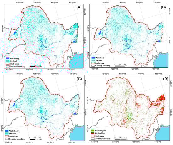
Figure 5.
Geographical distributions of wetlands and waterbody on the CARB. (A) Wetland and water body in 1990; (B) Wetland and water body in 2000; (C). Wetland and water body in 2010; (D) Loss and gain of wetland during 1990–2010.
3.3. Temporal Changes of Wetlands and Oher Land Covers
The changes of spatial extents and areas of different land covers from 1990 to 2010 are presented in Table 5, Figure 6 and Figure 7. In 1990, the total CARB wetland area was about 89,432 km2, within which marsh, occupying approximately 93% of whole wetlands area, was the most common wetland type. The area of water body on the CARB was 17,964 km2. On the CARB, woodland, dry farmland and grassland were the most common types, occupying 42%, 36% and 10%, respectively.
Table 5.
Areal extents and changes of wetland and other land covers on the CARB.
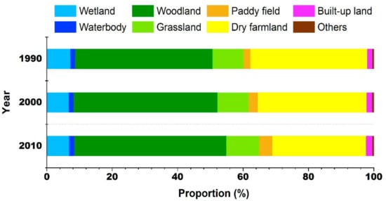
Figure 6.
Areal proportions of different land covers in 1990, 2000, and 2010 of the CARB.
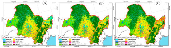
Figure 7.
Spatial pattern of land covers of the CARB in 1990 (A), 2000 (B), and 2010 (C).
The most significant wetland loss was shown from 1990 to 2000 with an area decline of 10,806 km2 (12%). Dry farmland area continually and strongly decreased from 440,395 km2 in 1990 to 388,111 km2 in 2000. In contrast, woodland and paddy field showed continual increases from 1990 to 2000. The results of grassland, built-up land and waterbody showed slight variability from 1990 to 2010. From 2000 to 2010, the CARB lost 4% of its total wetlands (3155 km2). About 18% of dry farmland on the CARB vanished between 2000 and 2010; a linear trend showed that the average rate of loss reached 7139 km2/y. In contrast, an increasing trend was observed for paddy field, and the total paddy field area increased by 38%.
3.4. Conversions between Wetland and Anthropogenic Land Covers
The conversions between wetland and other land covers were shown in Table 6. We discovered that nearly 85% of lost wetlands were converted to anthropogenic land covers between 1990 and 2000. These losses, which include 8479 km2 of wetlands to dry farmlands and about 2030 km2 of wetlands to paddy fields, however, are partially offset by gains of nearly 330 km2 from dry farmlands and paddy fields, to total net losses of around 10,366 km2.
Table 6.
Areal extents and conversions between wetland and other land covers.
The wetlands conversion ratio then gradually dropped, with a total loss rate of 58% from 2000 to 2010. We demonstrated that agricultural exploitation was the chief contributor to the lost wetlands on the CARB. From 2000 to 2010, about 1867 km2 of the wetlands had been modified to dry farmlands, and about 1368 km2 of the wetlands was occupied by paddy fields. Although the rate of wetland conversion has slowed between 2000 and 2010, wetland losses continued to out-distance wetland gains.
4. Discussion
4.1. Advantages and Uncertainties of the Migrated Training Samples
We adopted a robust methodology to migrate 2018′s training samples to historical time periods (the years of 2010, 2000, and 1990). The method used spectral similarity and spectral distance to determine whether a training sample of a reference year can be migrated to a target year. The accuracy assessments confirmed that the training sample migration method was successfully implemented in mapping historical land covers of the CARB. To our knowledge, the successful implementations could be attributed to two aspects, namely, the good performance of spectral similarity and spectral distance and the powerful computing abilities of the GEE platform. Firstly, this study chose images from the same seasons of different time periods (year of 2010, 2000, and 1990), and calculated both similarity and distance of the spectra to ensure unchanged samples. Secondly, the GEE platform provides full-storage dataset, meanwhile it offers online code editor and shares super computing power. For this study, over 20,000 training samples were migrated to the year of 2010, 2000, and 1990 by the GEE platform. The processes were rapid and robust.
Errors and limitations of the migrated training samples were caused mainly by the uncertainties of the image conditions. For example, if the image was captured after heavy rain, the spectra of grassland and woodland could be simple to wetlands, which, thus, led to further misclassifications. By building two season spectral curves, we tried to reduce such uncertainties as much as possible. However, for a broad scale such as the CARB, uncertainties could not be avoided completely.
4.2. Lost and Conservation of Wetlands on the CARB
As shown in Figure 7 and Table 6, conversions of wetland and other land covers, both direct and indirect factors caused the serious losses of wetlands on the CARB during the historical time periods (1990–2010). As is known, the study area is one of the major grain producing areas in China. Therefore, for a long time, two primary threats to wetlands on the CARB were agricultural development and population increase [7,8,43]. According to Table 4, dry farmland and paddy fields exploitations have occupied a large area of wetlands. Mao et al. [44] pointed out that 86% of the natural wetland losses in North-east China from 1990 to 2010 arose from agricultural encroachment. It has also been shown by previous studies that in the Songnen and Sanjiang Plain, most farmlands were developed by reclaimed natural wetlands [7,45]. Particularly during the implementation of the “Comprehensive Agricultural Development Project” by the Chinese government (from the mid-1980s to 2000), large areas of swamps had been converted into farmland [46,47]. From the mid-1980s to 2000, for instance, in the Sanjiang Plain, cropland added up to 10,400 km2 and most of these new cropland emerged from wetland conversion [7,48].
The construction of the project has also significantly affected the wetlands on the CARB [45]. As regions being faced with flood disaster on the CARB, a lot of embankments and reservoirs have been constructed. Fragmentation of wetlands were also caused by built-up land development.
Moreover, some indirect factors could also lead to significant wetland degradation, such as climate change and agricultural irrigation from wetland water [2,49], which would contribute to a decrease in the amount of wetland water and further degradation of marsh into grassland [49].
According to our results, between 1990 and 2010, the net loss of wetlands in the whole basin was 16%. Some previous studies of wetlands on the CARB also indicated the same trend of wetland losses. Liu et al. [50] showed that wetlands in the Heilongjiang province reduced over 13,000 km2 from 1990 to 2014, accounting for one quarter of 1990’s total wetlands. As Chen et al. [46] reported, from 1990 to 2015, Sanjiang Plain lost approximately 30% of wetlands, and at the same time, in the Songnen Plain saw 12% of wetlands lost. As Tian et al. [51] reported between 2000 and 2015, about 10% of wetlands in the Songnen Plain had disappeared. Jia et al. [2] indicated that floodplain wetland on the CARB had losses of 25% from 1990 to 2018.
As is shown in Table 5, Figure 6 and Figure 7, from 1990 to 2010, the tendency of wetland loss has slowed down. In the meantime, wetland rehabilitation from cropland, (i.e., dry farmland and paddy field) was enhanced. From 1990 to 2000 and 2000 to 2010, there were 330.43 km2 and 528.86 km2 of wetlands rehabilitated from croplands, respectively. A series of projects promoted these positive effects, which relied on Chinese and local governments’ efforts, even transnational cooperation. For example, the 2002–2030 National Wetland Conservation Program was approved in 2003 by the central government. This program aimed to establish natural reserves and restore wetlands [52]. To date, on the CARB there are more than 40 national wetland reserves, these reserves strengthen wetland conservation projects [53]. On another positive aspect, in 2011 Russia and China adopted the “Russian–Chinese Strategy for Development of Transboundary Network of Protected Areas in the Amur River Basin for the period till 2020”, which stressed the inventory and protection of wetlands as the first priority. The strategy also provided a basis for improving cooperation between different conservation agencies and the establishment of transboundary nature reserves [54]. However, the areal extent is still shrinking in the CARB, even though numerous conservation and restoration measures have been taken. Anthropogenic factors including population increase and socioeconomic development become main reasons for these shrinkages [46]. Therefore, further sustainable managements are still necessary to promote conservation and rehabilitation efforts for wetland on the CARB [44].
5. Conclusions
In this study, we adopted a convenient and robust training sample migration method along with the RF classifier to classify wetland and other land cover types on the CARB using two seasons’ worth of Landsat image collections. Resultantly, a 30-m resolution dataset for the CARB containing historical spatial distribution information of wetlands and other land covers in 1990, 2000, and 2010 was produced. The basic idea of the training sample migration is to compare the spectral similarity and spectral distance to determine whether a reference sample could be used as a training sample in a target year. Accuracy assessments showed high producer’s and user’s accuracies for all maps in the dataset. This success owed to the robustness and sufficiency of the training sample migration and RF classification, combined with super computing power and the complete storage of Landsat data of the GEE platform. According to the dynamics and conversions reflected by the resultant dataset, the area of wetland reduced from 89,432 km2 to 75,061 km2 from 1990 to 2010, with a net loss of 16%. At the same time, a majority of these reduced wetlands were converted into dry farmland and paddy field, especially in the Songnen and Sanjiang plains, which suggested that agricultural activities are the main cause of wetland loss. The dataset obtained by this study can provide reliable information for wetland management and socio-economic sustainable development in the CARB, and could be a reference for other related research.
Author Contributions
Conceptualization, Q.Z. and M.J.; methodology, Q.Z. and Y.W.; software, X.L.; investigation, M.J. and X.L.; writing—review and editing, Q.Z., M.J., J.L., H.P., Y.W. and X.L. All authors have read and agreed to the published version of the manuscript.
Funding
This research was funded by the National Key Research and Development Program of China (No. 2017YFC0404503), National Natural Science foundation of China (No. 41601529), and the Youth Innovation Promotion Association of Chinese Academy of Sciences (No. 2021227), the Open Fund of State Laboratory of Information Engineering in Surveying, Mapping and Remote Sensing, Wuhan University (Grant No. 19I02), the Science and Technology Development Program of Jilin Province (No. 20200301014RQ).
Institutional Review Board Statement
Not applicable.
Informed Consent Statement
Not applicable.
Data Availability Statement
The data presented in this study are available on request from the corresponding author. The data are not publicly available due to the funding project is not finished yet.
Acknowledgments
The authors thank Xin Wen at Jilin University and Rong Zhang at Northeast Institute of Geography and Agroecology, CAS for their advice on revising the manuscript. Lastly the authors would like to acknowledge the anonymous reviewers and editors whose thoughtful comments helped to improve this manuscript.
Conflicts of Interest
The authors declare no conflict of interest.
References
- Mao, D.; Wang, Z.; Wu, J.; Wu, B.; Zeng, Y.; Song, K.; Yi, K.; Luo, L. China’s wetlands loss to urban expansion. Land Degrad. Dev. 2018, 29, 2644–2657. [Google Scholar] [CrossRef]
- Jia, M.; Mao, D.; Wang, Z.; Ren, C.; Zhu, Q.; Li, X.; Zhang, Y. Tracking long-term floodplain wetland changes: A case study in the China side of the Amur River Basin. Int. J. Appl. Earth Obs. Geoinf. 2020, 92, 102185. [Google Scholar] [CrossRef]
- Asselen, S.; Verburg, P.H.; Vermaat, J.E.; Janse, J.H. Drivers of wetland conversion: A global meta-analysis. PLoS ONE 2013, 8. [Google Scholar] [CrossRef]
- Mao, D.; Tian, Y.; Wang, Z.; Jia, M.; Du, J.; Song, C. Wetland changes in the Amur River Basin: Differing trends and proximate causes on the Chinese and Russian sides. J. Environ. Manag. 2021, 280, 111670. [Google Scholar] [CrossRef] [PubMed]
- Sokolova, G.V.; Verkhoturov, A.L.; Korolev, S.P. Impact of Deforestation on Streamflow in the Amur River Basin. Geosciences 2019, 9, 262. [Google Scholar] [CrossRef]
- Chu, H.; Venevsky, S.; Wu, C.; Wang, M. NDVI-based vegetation dynamics and its response to climate changes at Amur-Heilongjiang River Basin from 1982 to 2015. Sci. Total Environ. 2019, 650, 2051–2062. [Google Scholar] [CrossRef] [PubMed]
- Wang, Z.M.; Song, K.S.; Ma, W.H.; Ren, C.Y.; Zhang, B.; Liu, D.W.; Chen, J.M.; Song, C.C. Loss and Fragmentation of Marshes in the Sanjiang Plain, Northeast China, 1954–2005. Wetlands 2011, 31, 945–954. [Google Scholar] [CrossRef]
- Zou, Y.; Wang, L.; Xue, Z.; Mingju, E.; Jiang, M.; Lu, X.; Yang, S.; Shen, X.; Liu, Z.; Sun, G.; et al. Impacts of Agricultural and Reclamation Practices on Wetlands in the Amur River Basin, Northeastern China. Wetlands 2018, 38, 383–389. [Google Scholar] [CrossRef]
- Jia, M.; Wang, Z.; Zhang, Y.; Mao, D.; Wang, C. Monitoring loss and recovery of mangrove forests during 42 years: The achievements of mangrove conservation in China. Int. J. Appl. Earth Obs. Geoinf. 2018, 73, 535–545. [Google Scholar] [CrossRef]
- Mao, D.; Wang, Z.; Du, B.; Li, L.; Tian, Y.; Jia, M.; Zeng, Y.; Song, K.; Jiang, M.; Wang, Y. National wetland mapping in China: A new product resulting from object-based and hierarchical classification of Landsat 8 OLI images. Int. J. Photogramm. Remote Sens. 2020, 164, 11–25. [Google Scholar] [CrossRef]
- Jia, M.; Wang, Z.; Wang, C.; Mao, D.; Zhang, Y. A New Vegetation Index to Detect Periodically Submerged Mangrove Forest Using Single-Tide Sentinel-2 Imagery. Remote Sens. 2019, 11, 2043. [Google Scholar] [CrossRef]
- Ji, L.; Gong, P.; Geng, X.; Zhao, Y. Improving the Accuracy of the Water Surface Cover Type in the 30 m FROM-GLC Product. Remote Sens. 2015, 7, 13507–13527. [Google Scholar] [CrossRef]
- Ji, C.; Zhang, Y.; Cheng, Q.; Tsou, J.; Jiang, T.; San Liang, X. Evaluating the impact of sea surface temperature (SST) on spatial distribution of chlorophyll-a concentration in the East China Sea. Int. J. Appl. Earth Obs. Geoinf. 2018, 68, 252–261. [Google Scholar] [CrossRef]
- Liu, M.; Zhang, H.; Lin, G.; Lin, H.; Tang, D. Zonation and directional dynamics of mangrove forests derived from time-series satellite imagery in Mai Po, Hong Kong. Sustainability 2018, 10, 1913. [Google Scholar] [CrossRef]
- Zhang, Y.; Huang, Z.; Fu, D.; Tsou, J.Y.; Jiang, T.; San Liang, X.; Lu, X. Monitoring of chlorophyll-a and sea surface silicate concentrations in the south part of Cheju island in the East China sea using MODIS data. Int. J. Appl. Earth Obs. Geoinf. 2018, 67, 173–178. [Google Scholar] [CrossRef]
- Belgiu, M.; Drăguţ, L. Random forest in remote sensing: A review of applications and future directions. Int. J. Photogramm. Remote Sens. 2016, 114, 24–31. [Google Scholar] [CrossRef]
- Gibson, R.; Danaher, T.; Hehir, W.; Collins, L. A remote sensing approach to mapping fire severity in south-eastern Australia using sentinel 2 and random forest. Remote Sens. Environ. 2020, 240, 111702. [Google Scholar] [CrossRef]
- Gislason, P.O.; Benediktsson, J.A.; Sveinsson, J.R. Random Forests for land cover classification. Pattern Recogn. Lett. 2006, 27, 294–300. [Google Scholar] [CrossRef]
- Murray, N.J.; Phinn, S.R.; DeWitt, M.; Ferrari, R.; Johnston, R.; Lyons, M.B.; Clinton, N.; Thau, D.; Fuller, R.A. The global distribution and trajectory of tidal flats. Nature 2019, 565, 222–225. [Google Scholar] [CrossRef] [PubMed]
- Huang, H.; Wang, J.; Liu, C.; Liang, L.; Li, C.; Gong, P. The migration of training samples towards dynamic global land cover mapping. Int. J. Photogramm. Remote Sens. 2020, 161, 27–36. [Google Scholar] [CrossRef]
- Foody, G.; Arora, M. An evaluation of some factors affecting the accuracy of classification by an artificial neural network. Int. J. Remote Sens. 1997, 18, 799–810. [Google Scholar] [CrossRef]
- Li, C.; Wang, J.; Wang, L.; Hu, L.; Gong, P. Comparison of classification algorithms and training sample sizes in urban land classification with Landsat thematic mapper imagery. Remote Sens. 2014, 6, 964–983. [Google Scholar] [CrossRef]
- Radoux, J.; Lamarche, C.; Van Bogaert, E.; Bontemps, S.; Brockmann, C.; Defourny, P. Automated training sample extraction for global land cover mapping. Remote Sens. 2014, 6, 3965–3987. [Google Scholar] [CrossRef]
- Dong, J.; Xiao, X.; Menarguez, M.A.; Zhang, G.; Qin, Y.; Thau, D.; Biradar, C.; Moore, B. Mapping paddy rice planting area in northeastern Asia with Landsat 8 images, phenology-based algorithm and Google Earth Engine. Remote Sens. Environ. 2016, 185, 142–154. [Google Scholar] [CrossRef]
- Wang, C.; Jia, M.; Chen, N.; Wang, W. Long-Term Surface Water Dynamics Analysis Based on Landsat Imagery and the Google Earth Engine Platform: A Case Study in the Middle Yangtze River Basin. Remote Sens. 2018, 10, 1635. [Google Scholar] [CrossRef]
- Simonov, E.A.; Dahmer, T.D. Amur-Heilong River Basin Reader; Ecosystems Hongkong: Hongkong, China, 2008. [Google Scholar]
- Jia, H.; Pan, D.; Zhang, W. Health Assessment of Wetland Ecosystems in the Heilongjiang River Basin, China. Wetlands 2015, 35, 1185–1200. [Google Scholar] [CrossRef]
- Chen, X.; Chen, J.; Shi, Y.; Yamaguchi, Y. An automated approach for updating land cover maps based on integrated change detection and classification methods. Int. J. Photogramm. Remote Sens. 2012, 71, 86–95. [Google Scholar] [CrossRef]
- Carvalho Junior, O.A.; Guimarães, R.F.; Gillespie, A.R.; Silva, N.C.; Gomes, R.A. A new approach to change vector analysis using distance and similarity measures. Remote Sens. 2011, 3, 2473–2493. [Google Scholar] [CrossRef]
- Kruse, F.A.; Lefkoff, A.; Boardman, J.; Heidebrecht, K.; Shapiro, A.; Barloon, P.; Goetz, A. The spectral image processing system (SIPS)—interactive visualization and analysis of imaging spectrometer data. Remote Sens. Environ. 1993, 44, 145–163. [Google Scholar] [CrossRef]
- Breiman, L. Random Forests. Mach. Learn. 2001, 45, 5–32. [Google Scholar] [CrossRef]
- Rodriguez-Galiano, V.F.; Ghimire, B.; Rogan, J.; Chica-Olmo, M.; Rigol-Sanchez, J.P. An assessment of the effectiveness of a random forest classifier for land-cover classification. Int. J. Photogramm. Remote Sens. 2012, 67, 93–104. [Google Scholar] [CrossRef]
- Pal, M. Random forest classifier for remote sensing classification. Int. J. Remote Sens. 2005, 26, 217–222. [Google Scholar] [CrossRef]
- Trigila, A.; Iadanza, C.; Esposito, C.; Scarascia-Mugnozza, G. Comparison of Logistic Regression and Random Forests techniques for shallow landslide susceptibility assessment in Giampilieri (NE Sicily, Italy). Geomorphology 2015, 249, 119–136. [Google Scholar] [CrossRef]
- Pal, M.; Mather, P.M. An assessment of the effectiveness of decision tree methods for land cover classification. Remote Sens. Environ. 2003, 86, 554–565. [Google Scholar] [CrossRef]
- Tucker, C.J. Red and photographic infrared linear combinations for monitoring vegetation. Remote Sens. Environ. 1979, 8, 127–150. [Google Scholar] [CrossRef]
- Huete, A.; Liu, H.; Batchily, K.; Van Leeuwen, W. A comparison of vegetation indices over a global set of TM images for EOS-MODIS. Remote Sens. Environ. 1997, 59, 440–451. [Google Scholar] [CrossRef]
- McFeeters, S.K. The use of the Normalized Difference Water Index (NDWI) in the delineation of open water features. Int. J. Remote Sens. 1996, 17, 1425–1432. [Google Scholar] [CrossRef]
- Xu, H. Modification of normalised difference water index (NDWI) to enhance open water features in remotely sensed imagery. Int. J. Remote Sens. 2006, 27, 3025–3033. [Google Scholar] [CrossRef]
- Jia, M.; Wang, Z.; Mao, D.; Ren, C.; Wang, C.; Wang, Y. Rapid, robust, and automated mapping of tidal flats in China using time series Sentinel-2 images and Google Earth Engine. Remote Sens. Environ. 2021, 255, 112285. [Google Scholar] [CrossRef]
- Rogers, A.; Kearney, M. Reducing signature variability in unmixing coastal marsh Thematic Mapper scenes using spectral indices. Int. J. Remote Sens. 2004, 25, 2317–2335. [Google Scholar] [CrossRef]
- Olofsson, P.; Foody, G.M.; Herold, M.; Stehman, S.V.; Woodcock, C.E.; Wulder, M.A. Good practices for estimating area and assessing accuracy of land change. Remote Sens. Environ. 2014, 148, 42–57. [Google Scholar] [CrossRef]
- Yan, F. Large-Scale Marsh Loss Reconstructed from Satellite Data in the Small Sanjiang Plain since 1965: Process, Pattern and Driving Force. Sensors 2020, 20, 1036. [Google Scholar] [CrossRef] [PubMed]
- Mao, D.; Luo, L.; Wang, Z.; Wilson, M.C.; Zeng, Y.; Wu, B.; Wu, J. Conversions between natural wetlands and farmland in China: A multiscale geospatial analysis. Sci. Total Environ. 2018, 634, 550–560. [Google Scholar] [CrossRef] [PubMed]
- Yu, X.; Ding, S.; Zou, Y.; Xue, Z.; Lyu, X.; Wang, G. Review of Rapid Transformation of Floodplain Wetlands in Northeast China: Roles of Human Development and Global Environmental Change. Chin. Geogr. Sci. 2018, 28, 654–664. [Google Scholar] [CrossRef]
- Chen, H.; Zhang, W.; Gao, H.; Nie, N. Climate Change and Anthropogenic Impacts on Wetland and Agriculture in the Songnen and Sanjiang Plain, Northeast China. Remote Sens. 2018, 10, 356. [Google Scholar] [CrossRef]
- Mao, D.; Wang, Z.; Wu, B.; Zeng, Y.; Luo, L.; Zhang, B. Land degradation and restoration in the arid and semiarid zones of China: Quantified evidence and implications from satellites. Land Degrad. Dev. 2018, 29, 3841–3851. [Google Scholar] [CrossRef]
- Liu, H.; Zhang, S.; Li, Z.; Lu, X.; Yang, Q. Impacts on wetlands of large-scale land-use changes by agricultural development: The small Sanjiang Plain, China. AMBIO J. Hum. Environ. 2004, 33, 306–310. [Google Scholar] [CrossRef]
- Zhang, J.; Ma, K.; Fu, B. Wetland loss under the impact of agricultural development in the Sanjiang Plain, NE China. Environ. Monit. Assess. 2010, 166, 139–148. [Google Scholar] [CrossRef] [PubMed]
- Liu, W.; Guo, Z.; Jiang, B.; Lu, F.; Wang, H.; Wang, D.; Zhang, M.; Cui, L. Improving wetland ecosystem health in China. Ecol. Indic. 2020, 113, 106184. [Google Scholar] [CrossRef]
- Tian, Y.; Wang, Z.; Mao, D.; Li, L.; Liu, M.; Jia, M.; Man, W.; Lu, C. Remote Observation in Habitat Suitability Changes for Waterbirds in the West Songnen Plain, China. Sustainability 2019, 11, 1552. [Google Scholar] [CrossRef]
- Wang, Z.; Wu, J.; Madden, M.; Mao, D. China’s Wetlands: Conservation plans and policy impacts. Ambio 2012, 41, 782–786. [Google Scholar] [CrossRef] [PubMed]
- Turner, R.K.; Van Den Bergh, J.C.; Söderqvist, T.; Barendregt, A.; Van Der Straaten, J.; Maltby, E.; Van Ierland, E.C. Ecological-economic analysis of wetlands: Scientific integration for management and policy. Ecol. Econ. 2000, 35, 7–23. [Google Scholar] [CrossRef]
- Egidarev, E.; Simonov, E.; Darman, Y. Amur-Heilong River Basin: Overview of Wetland Resources. In The Wetland Book; Springer: Berlin/Heidelberg, Germany, 2016; pp. 1–15. [Google Scholar]


Publisher’s Note: MDPI stays neutral with regard to jurisdictional claims in published maps and institutional affiliations. |
© 2021 by the authors. Licensee MDPI, Basel, Switzerland. This article is an open access article distributed under the terms and conditions of the Creative Commons Attribution (CC BY) license (https://creativecommons.org/licenses/by/4.0/).