A Constrained Sparse-Representation-Based Spatio-Temporal Anomaly Detector for Moving Targets in Hyperspectral Imagery Sequences


College of Electronic Science and Technology, National University of Defense Technology, Changsha 410073, China
*
Author to whom correspondence should be addressed.
†
These authors contributed equally to this work.
Remote Sens. 2020, 12(17), 2783; https://doi.org/10.3390/rs12172783
Submission received: 5 August 2020
/
Revised: 22 August 2020
/
Accepted: 25 August 2020
/
Published: 27 August 2020
(This article belongs to the Special Issue Advances in Hyperspectral Data Exploitation)
Abstract
:At present, small dim moving target detection in hyperspectral imagery sequences is mainly based on anomaly detection (AD). However, most conventional detection algorithms only utilize the spatial spectral information and rarely employ the temporal spectral information. Besides, multiple targets in complex motion situations, such as multiple targets at different velocities and dense targets on the same trajectory, are still challenges for moving target detection. To address these problems, we propose a novel constrained sparse representation-based spatio-temporal anomaly detection algorithm that extends AD from the spatial domain to the spatio-temporal domain. Our algorithm includes a spatial detector and a temporal detector, which play different roles in moving target detection. The former can suppress moving background regions, and the latter can suppress non-homogeneous background and stationary objects. Two temporal background purification procedures maintain the effectiveness of the temporal detector for multiple targets in complex motion situations. Moreover, the smoothing and fusion of the spatial and temporal detection maps can adequately suppress background clutter and false alarms on the maps. Experiments conducted on a real dataset and a synthetic dataset show that the proposed algorithm can accurately detect multiple targets with different velocities and dense targets with the same trajectory and outperforms other state-of-the-art algorithms in high-noise scenarios.
1. Introduction
With the development of optical sensor technology, hyperspectral imagery (HSI) has been dramatically improved in recent years, and HSI sequences are more available in the real world. Because of adequate spectral information with dozens or hundreds of spectrum bands, the HSI detection technique can find and distinguish dim targets, which are unobservable in the visible or infrared images, and has promising prospects in military, security, satellite surveillance, disaster monitoring, and other applications [1]. According to whether prior target spectral information is utilized, the HSI detection technique can be mainly divided into target detection [2,3,4] and anomaly detection. Due to factors such as camera angle, illumination, atmosphere, and sensor spatial resolution, it is common in HSI that the same object has different spectra. Besides, no prior target spectrum is available for most of the moving target detection scenes. Therefore, current hyperspectral moving target detection technologies [5,6,7,8,9,10,11,12] are mainly based on anomaly detection.
Traditional single-frame anomaly detection is usually accomplished by detecting irregular deviations between the test pixel and background pixels in a hyperspectral image. Designed to detect the presence of a dim target in a multi-band image, the Reed–Xiaoli (RX) algorithm [13] assumes that the global background spectra obey a multivariate Gaussian distribution and applies the Mahalanobis distance to identify anomaly spectra. To solve the problem that the Gaussian distribution is not applicable to the non-stationary global background, the local version of RX [14] divides the local neighborhood of the test pixel into potential regions and background regions by dual-windows and replaces global statistics with local statistics. The Quasi-local-RX (QLRX) algorithm [15] improves point-target detection by utilizing local and global statistics simultaneously. The kernel RX (KRX) algorithm [16], a nonlinear version of RX, maps spectra into a more high-dimensional characteristic space through a kernel function and outperforms the original RX detector in military target and mine detection. The cluster KRX (CKRX) algorithm [17] improves the performance of KRX by replacing background pixels with cluster centers. Support vector data description (SVDD) algorithms [18,19] also determine anomalies in a high-dimensional characteristic space by building a minimal enclosing hypersphere around local background pixels. Sparse representation (SR)-based algorithms [20,21,22,23,24,25,26,27] have made significant progress in anomaly detection in recent years. These algorithms usually assume that background pixels can be presented as linear combinations of the surrounding background, and anomaly pixels cannot. The collaborative representation (CR)-based algorithm [22] adopts -norm minimization to reinforce the collaboration of background representation and is superior to RX and its improved algorithms. To realize the detection of dense small targets, the constrained sparse representation (CSR)-based algorithm [23] imposes two constraints on abundance vectors and can remove anomalous atoms from the local background dictionary. Because background pixels and target pixels are considered low rank and sparse, respectively, low-rank and sparse matrix decomposition-based algorithms [28,29,30] have also received widespread attention in anomaly detection.
When a hyperspectral staring camera is continuously imaging at short intervals, anomaly detectors can output detection maps in succession. Usually, anomaly detection maps of a hyperspectral imagery sequence can be regarded as an infrared image sequence. Therefore, multi-frame infrared detection or tracking algorithms can be used to detect or track dim moving targets on these maps. Rotman et al. combined hyperspectral target detection and infrared target tracking for the first time [5,6,7]. They transformed each HSI into a two-dimensional anomaly detection map and then utilized a variance filter (VF) [31] to detect targets moving at subpixel velocity. Besides, Duran et al. focused on tracking small dense objects, such as pedestrians or vehicles, from airborne platforms [8,9,10]. They adopted endmember techniques to detect subpixel targets and estimated the motion parameters of targets under the framework of the Bayesian filter. Wang et al. proposed a novel temporal anomaly detector in dim moving target detection, which extracts the local spatial background in the previous frame to mine the singularity of the test pixel [11]. Combining the traditional single-frame detection with their proposed temporal detection can effectively reduce temporal noise clutter. Then, Wang et al. introduced a simplified VF to calculate a trajectory history map in the literature [12]. The fusion of the spatial detection map, the temporal detection map, and the trajectory history map (STH) is superior to previous moving target detection algorithms in hyperspectral imagery sequences.
In summary, current anomaly detection algorithms for moving targets still only utilize the spatial neighborhood background of the current frame or the previous frame. However, static or non-moving objects for which the spectra are different from neighborhoods can be regarded as anomaly targets by these detection algorithms. Temporal profile filtering algorithms can detect moving targets, but ask for prior information about speed. Besides, detecting targets in complex motion, such as multiple targets at different velocities and dense targets on the same trajectory, is still a challenge for temporal profile filtering-based algorithms [5,6,7,11]. To solve these problems, we propose a CSR-based spatio-temporal anomaly detector (CSR-ST), sufficiently employing temporal spectral information in HSI sequences. Unlike hyperspectral change detection (CD) [32,33], which detects anomaly regions under diurnal and seasonal changes, moving target detection asks for a very short interval between frames. This means that camera angle, illumination, weather, and other imaging conditions are almost unchanged in adjacent frames. After frame registration, the spectrum of the same pixel can be regarded as a mixture of spectra in a small local region, only affected by the temporal clutter in different frames. Based on this assumption, we propose a novel temporal anomaly detection framework that calculates the anomaly score of the test pixel employing its former spectra. In our previous work [23], the CSR detector was based on the assumption that a background pixel can be linearly represented by the endmembers present in its spatial neighborhood while an anomaly pixel cannot. Compared to background spectra in the spatial neighborhood, the former spectra of the test pixel in previous frames can provide more pure background endmembers to represent the current spectrum. Therefore, the CSR-based temporal detector has a better ability to recover the test background pixel than the CSR-based spatial detector. Besides, the temporal detector has two insurances to construct a pure temporal background dictionary for the test pixel. The first insurance is to remove potential target spectra from the candidate set of the temporal background dictionary based on spatial detection results. The other insurance is to automatically remove anomaly atoms from the background dictionary when the corresponding abundances are higher than a given upper bound and then solve the model with the new background dictionary. Non-homogeneous background pixels or stationary objects can turn into false alarms in the single-frame detection, while the temporal detector is mainly sensitive to moving targets. However, when some background regions move in the imaging scene, the temporal detector can regard them as targets and be inferior to the spatial detector. The fusion of the spatial detection map and the temporal detection map combines the advantages of the two detectors and can suppress the background and stationary objects. The main contributions of this article are summarized as follows.
- A novel hyperspectral spatio-temporal anomaly detection algorithm is proposed. Compared to traditional anomaly detection algorithms, the proposed algorithm utilizes the temporal spectral information and extends the CSR algorithm from the spatial domain to the spatio-temporal domain. The spatial detector and the temporal detector play different roles in moving target detection. The former can suppress moving background regions, and the latter can suppress non-homogeneous background and stationary objects. To the best of our knowledge, no literature has introduced the historical spectra of the test pixel to construct the temporal background set in anomaly detection yet.
- In the CSR-based temporal detection, there are two procedures to purify the background dictionary. The purification procedures can improve the ability of the temporal detector to detect multiple targets in complex motion situations, such as multiple targets with different velocities and dense targets with the same trajectory.
- An iterative smoothing filter is executed on both spatial and temporal detection maps to suppress the background clutter. Furthermore, the filter can strengthen the detection performance for slow-moving area targets.
The rest of this article is organized as follows. The CSR detector and its kernel version are introduced in Section 2. The proposed CSR-ST algorithm is described in Section 3. The experiments conducted on a real dataset and a synthetic dataset are presented in Section 4, followed by the conclusions in Section 5.
2. Related Work
SR-based anomaly detection algorithms usually assume that a background pixel can exist in a low-dimensional subspace spanned by surrounding background pixels. Meanwhile, anomaly pixels cannot be represented as a sparse linear mixture of background spectra. Suppose is the test pixel, which has N spectral bands, and is the background dictionary, which has M atoms; the competing hypotheses for the SR-based algorithms are:
where , is defined as a sparse vector for which each item is the abundance of the correlated atom in and is defined as a random noise item.
Usually, the sparse vector has a sparsity constraint imposed in SR-based detection, where K is a sparsity parameter. However, if there is no constraint on each abundance item in , anomaly pixels can also be linear mixtures of the background dictionary on account of abundance items less than zero. The linear spectral mixture model (LMM) [34] supposes that the abundance vector of a mixed pixel should satisfy a sum-to-one constraint:
and a non-negativity constraint:
The CSR algorithm introduces Equations (2) and (3) into the SR model, and the minimizing problem of CSR can be expressed as:
where represents an vector for which each item is one. The objective function can be converted to:
Note that is a constant and can be removed. If the test pixel is anomalous and the background dictionary contains a few anomaly pixels, the corresponding entries of can be enormous, resulting in a small reconstitution residual. To avoid missing alarms, an adequately tiny constant C is introduced as an upper limit of , and Equation (4) can be transformed as:
where . According to the Karush–Kuhn–Tucker conditions [35], the constraint in Equation (4) can be removed in Equation (6).
When abnormal pixels are tested, the abundances correlated with similar anomalous atoms can reach the maximum. Accordingly, the atoms for which the abundances are C have a significant possibility of being anomalies and should be eliminated from the background dictionary. A pure dictionary can be built by the remaining atom. With the constraint and , reconstruction residuals of anomalous test pixels will be significantly higher than those in the first reconstruction and can be regraded as anomaly scores.
where is the approximately calculated sparse vector without anomalous atoms in the background dictionary .
Given secondary or multiple scattering in the atmosphere, spectrum mixing usually is a nonlinear process [36]. The kernel methods map the original data into a more high-dimensional characteristic space via nonlinear functions and then achieve linear partition of the linearly inseparable data [37]. Skillfully, the inner product in the characteristic space can be replaced by:
where is a nonlinear function, and are the original data, and k is the kernel function. The kernel CSR (KCSR) algorithm introduces the kernel method and adopts the Gaussian radial basis function kernel:
The optimal problem is replaced by:
where is an Gram matrix for which the i-th row and j-th column item . and can also be replaced by:
Likewise, the atoms for which abundances are C are removed, and then, a pure background dictionary is used to solve Equation (10). Therefore, the anomaly score can be replaced by:
where r is the approximate error and and are both solved by .
3. Spatio-Temporal Anomaly Detection for Moving Targets
In this section, a novel CSR-based spatio-temporal anomaly algorithm is proposed to detect dim moving targets accurately in HSI sequences. Our algorithm is divided into four steps, namely spatial anomaly detection, iterative smoothing filter, temporal anomaly detection, and spatial-temporal fusion. The spatial anomaly detection finds abnormal targets by utilizing the spectral information of the current frame. An iterative smoothing filter can reduce noise and false alarms in the time and space domains. Different from AD, CD, and the temporal detection [12] using the information between two adjacent frames, our proposed temporal anomaly detection constructs background dictionaries with the historical spectral curves of the test pixels. The proposed temporal anomaly detection explores anomaly characteristics in the time dimension and provides anomaly information different from that in the spatial detection. The fusion of spatial and temporal anomaly detection can explore the target information more comprehensively. The framework of the proposed CSR-ST algorithm is displayed in Figure 1.
3.1. Spatial Anomaly Detection
Let denote a hyperspectral cube collected in the current frame, where i is the current sequence number, and are defined as the space sizes of the cube, and N is the quantity of spectral bands. Dual concentric windows [38] are used to extract a spatial background dictionary for each pixel . The dual-windows are centered at each test pixel and divide the neighborhood into a potential target region and a background region. Pixels in the background region are selected as atoms to form a background dictionary . Then, the spatial anomaly score of the test pixel is solved by the CSR detector with the corresponding background dictionary . After all pixels on are detected in sequence, a two-dimensional spatial detection map is obtained:
3.2. Iterative Smoothing Filter
The spectra change with time due to the measurement noise, resulting in temporal fluctuation of anomaly scores. Meanwhile, spatial background clutter is also generated in the detection maps due to the fluctuation. The literature [17] has used a simple smoothing filter as a post-processing procedure to decrease false alarms and noise in detection maps. Inspired by [17], an iterative smoothing filter is adopted to reduce noise both in the spatial and temporal domains simultaneously.
To avoid the overall drift of anomaly scores on the spatial detection map caused by sudden changes in imaging conditions, Z-score normalization should be first performed:
In typical image preprocessing, and are the mean value and standard deviation of pixels in the whole image, respectively. However, because anomaly scores of anomalous pixels are much higher than those of background pixels on , it is more accurate to describe the distribution of by a truncated normal distribution or a half-normal distribution [39] rather than a normal distribution. Therefore, it is more reasonable to set and to the mean value and standard deviation of the collection of and its symmetric set about zero.
Then, an iterative smoothing operation is performed on to reduce spatial and temporal clutter:
where is the normalized spatial anomaly scores of , and are the smoothed spatial anomaly scores of and , respectively, denotes the spatial neighborhood used for smoothing, and and denote filter weights. When the first spatial detection map is smoothed, let . The latter part of Equation (15) is actually a spatial smoothing filter such as the mean filter or the Gaussian filter. Furthermore, one-dimensional denoising algorithms can also replace the temporal iterative smoothing part of Equation (15) to reduce temporal clutter. Compared to the original spatial detection map , background clutter and noise on are suppressed, and detection performance can be improved.
3.3. Temporal Anomaly Detection
Note that, using the dual-window strategy to select a background dictionary has several disadvantages. Firstly, the selection of an inappropriate dual-window size can cause the local background to be contaminated by target pixels in spatial anomaly detection. If the inner window of dual-windows is too small, the chosen local background of the test target pixel can contain some target pixels. Moreover, the contamination problem can also occur when multiple targets are densely distributed. Secondly, the spatial distributions of moving targets are usually unknown and change in the real world. Therefore, it is difficult to determine the optimal dual-window size to detect moving targets in advance. Thirdly, the performance of these algorithms still varies with the dual-window size, and the best performance of the dual-window-based AD algorithms is a local optimum. For instance, detection results can be further improved after combining with a weight matrix obtained by segmentation or clustering in the literature [40,41], where background pixels are assigned lower weight values. An interesting phenomenon is that the best local background of some detection algorithms for subpixel targets are eight neighborhoods [42], and large dual-windows are harmful to these algorithms. Fourthly, the dual-window-based spatial detection cannot eliminate motionless objects, the spectra of which are also different from the background spectra.
To accurately detect moving targets in HSI sequences, we propose a new approach for constructing background dictionaries of test pixels. Compared to hyperspectral CD, the interval between two contiguous frames in moving target detection is short; thus, the camera angle, illumination, weather, and other imaging conditions are almost unchanged. In this case, the spectrum of the same object in short HSI sequences can only be affected by the measured noise. Moreover, due to camera shake and the error of frame registration, the imaging space corresponding to the same pixel in the HSI moves back and forth in a local background region. Therefore, it can be assumed that the spectra of the same pixel in adjacent frames, , are a linear combination of the same set of endmembers. According to the LMM, the current pixel can be expressed as a linear combination of its former spectra :
where is defined as the former spectra matrix, is defined as the abundance vector, P is defined as the number of former spectra, and is defined as the noise item.
Equation (16) means that the test pixel and its former spectra can be also applied to the CSR detector. and can be considered to consist of the same set of background endmembers. In the spatial anomaly detection, the background dictionary constructed by the dual-window strategy contains some endmembers independent of . Compared to , is more suitable as a background dictionary for the CSR and KCSR detectors. In this subsection, temporal anomaly detection is defined as a method to calculate the anomaly scores of the test pixel in the current frame by using its former spectra . Because the positions of non-homogeneous background pixels or motionless objects are almost unchanged in the HSI after inter-frame registration, the temporal anomaly detection can avoid false alarms caused by these pixels.
However, is not a pure background dictionary sometimes. When the target is moving slowly, it takes more than one frame to pass through a pixel. In this case, if is a target pixel, it is possible that its former spectra are also target spectra. Besides, if the trajectories of moving targets intersect, the former spectra of pixels at the intersection can also be contaminated by targets. Therefore, we delete the abnormal atoms in based on the spatial anomaly detection results. and are defined as the number of atoms in the background dictionary and its candidate set, respectively. Specifically, for the test pixel in the current frame, smoothed spatial anomaly scores of its former spectra are sorted at first. In order from smallest to largest, the sort result is , where the subscripts are the sequence numbers. The smaller the spatial anomaly score is, the higher the probability that the corresponding former spectrum belongs to the background. Therefore, former spectra are selected to construct a pure background dictionary for the test pixel . Then, the minimizing problem in the CSR algorithm can be transformed as:
where . The background dictionary can be further purified by removing the atoms with . The temporal anomaly detection result of is transformed as:
where is the approximately calculated sparse vector without anomalous atoms in the background dictionary and is the -norm of the approximate error. Similarly, the KCSR algorithm can also be applied to the temporal anomaly detection. After all pixels on are detected in sequence, a two-dimensional temporal detection map is obtained.
The lower limit of the constraint parameter C is connected with the number of anomalous atoms in the background dictionary. To obtain a convenient setting of C in the spatial and temporal anomaly detection, C can be represented as:
where . If and , then the inequality constraint is invalid. To further explore the meaning of , two definitions are given as follows:
where is defined as the number of anomalous atoms and is defined as the abundance relevant to the anomaly endmember in the LMM of the l-th anomalous atom. In the hyperspectral AD, . We proofed a proposition of the parameter in the article [23]:
Proposition 1.
To delete all anomalous atoms from the background dictionary, ν must satisfy:
where is defined as the abundance relevant to the anomaly endmember in the LMM of the test pixel.
The proposition gives an intuitive interpretation of . When is larger than , all anomalous atoms can be deleted. Regardless of spatial detection or temporal detection, of the same test pixel is constant. Therefore, it is practicable to set to the same value in both detections. and in temporal detection can be set to values smaller than those in spatial detection by reducing the proportion of anomalous atoms in . One method is to enlarge , the size of . Another method is to decrease , the number of anomalous atoms, by enlarging the size of the candidate set or sample the former spectra at intervals before constructing . Through the above operations, the lower limit of in temporal detection is less than that in spatial detection. When is set to an excessively large value, numerous background atoms are exorbitantly deleted, resulting in slight degeneration in the ability of the CSR and KCSR algorithms to represent test background pixels. Therefore, should be a trade-off value between the inadequate deletion of anomalous atoms and unnecessary deletion in spatial detection. The same can cause the excessive deletion of atoms in temporal detection, but a large can avoid this situation.
3.4. Spatio-Temporal Fusion
Compared to the spatial anomaly detection, the temporal anomaly detection can suppress spatially non-homogeneous background pixels and stationary objects. Furthermore, compared to the temporal profile filtering algorithms, the proposed temporal anomaly detection can identify moving targets with different speeds simultaneously and is robust to the situation where multiple targets pass through the same trajectory one after the other. However, the temporal detection is inferior to the spatial detection in some situations. If there are some moving background pixels in the scene, such as clouds, temporal anomaly detection can judge them as targets. Besides, if the frame registration error is too large, the temporal background dictionary cannot describe the background accurately. To improve the stability and robustness of the detection algorithm, it is necessary to combine spatial and temporal detection results.
Before fusion, the filtering operation in Section 3.2 can also be performed on the temporal detection map . First, perform Z-score normalization on :
where and are set to the mean value and standard deviation of the collection of and its symmetric set about zero. Then, the same iterative smoothing operation as Equation (15) is performed on to reduce temporal clutter:
where is the normalized temporal anomaly scores of and and are the temporal spatial anomaly scores of and , respectively. The smoothed detection maps can be combined by the multiplication fusion strategy:
where and are the maximum values in and , and are the minimum values in and , the symbol ∘ denotes the Hadamard product, and is the fusion spatio-temporal detection map. The overall description of the proposed spatio-temporal anomaly detection is presented in Algorithm 1.
| Algorithm 1 CSR-based spatio-temporal anomaly detection for moving targets |
| Input: Hyperspectral sequences, dual-window size , temporal background dictionary size , candidate set size , parameter , and kernel parameter for KCSR. |
for each frame in the hyperspectral sequences do
|
| Output: Spatio-temporal anomaly detection map when . |
4. Experimental Results and Discussion
In the beginning of this section, a real HSI sequence dataset and a synthetic dataset are introduced. Subsequently, the capability of the proposed temporal anomaly detection with different background dictionary sizes and different spatial detection results is demonstrated in detail. Additionally, the proposed spatio-temporal anomaly detection is compared to several existing algorithms in the detection performance.
4.1. Datasets and Evaluation Metrics
The Cloud dataset is an HSI sequence under a complex cloudy background and was collected by the Interuniversity Microelectronics Centre of Beihang University with the xiSpec snapshot mosaic hyperspectral cameras [12]. The dataset has a spatial size of 409 × 216 pixels and 25 spectral bands including the 682–957 nm spectral region. The HSI sequence consists of 500 frames, where an aircraft (Target A) rises from the bottom of the imagery. Since the distance between the camera and the aircraft increases with the frames, the size of the aircraft decreases over time, 53 pixels in the 1st frame and 21 pixels in the 500th frame, resulting in a descending spectral difference from the background. However, because of the aircraft’s speed on HSIs also decreases, the number of frames that the aircraft needs to pass through a pixel increases. Three small flying targets (Target B, Target C, and Target D) with no more than 10 pixels exist in the 250th–393rd, 256th–363rd, and 417th–466th frames, respectively, and their velocities are all greater than 5 pixels per frame. As shown in Figure 2, there is a noise clutter in the cloudy background.
The synthetic dataset is based on the Terrain dataset acquired by the Hyperspectral Digital Image Collection Experiment sensor. The dataset has a spatial size of 180 × 180 pixels and 210 spectral bands including the 400–2500 nm spectral region, as shown in Figure 3a. The spatial resolution is 1 m, and the spectral resolution is 10 nm. The water absorption and high noise bands are deleted, and one-hundred sixty-two spectral bands are usable in the experiments. According to the LMM, synthetic targets can be added to the Terrain dataset by:
where is a pure target spectrum, is an original background spectrum, is a mixed target spectrum, is the added zero mean Gaussian noise vector, and is the target abundance to be set. Considering that the radiation response interval of the background varies with bands, Gaussian noise with different variance is added to each band of a hyperspectral cube. Noise intensity is adjusted by the signal-to-noise ratio (SNR), expressed in this dataset by:
where and are the variances of the background and noise in the l-th band. Three targets with a size of 5 × 5 pixels and a speed of 2 pixels per frame are added to the Terrain dataset and move 100 frames. The plane trajectories of targets are the same, and the distance between the two targets is ten frames. Considering that the boundaries between neighboring objects are often accompanied by severe spectral mixing in the real data, of 16 pixels on the periphery of targets is set to 10%, while that of 9 pixels in the center of targets is set to 40%. To explore the noise immunity of CSR-ST, the SNR is set to 20 dB, 10 dB, 5 dB, and 0 dB in turn. Figure 3b–f shows background spectra and mixed target spectra in different noise environments. With the decrease of SNR, the discriminability between background and mixed targets also decreases. When the SNR is 0 dB, background spectra and mixed target spectra are almost indistinguishable.
To evaluate anomaly detection performance, this article adopts the receiver operating characteristic (ROC) curve and the area under the ROC curve (AUC). The detection probability () and false alarm rate () are computed on a segmentation map, which is obtained on the detection map by a given threshold. After the threshold is iterated over, a set of and can be used to plot the ROC curve. An excellent detector has an upper left ROC curve [43]. However, the ROC curve can only qualitatively analyze detection performance. AUC [44] can give an intuitive and quantitative description and is calculated by several trapezoids:
where is defined as the l-th coordinate point and n is defined as the number of coordinate points constituting the curve. The closer to 1 AUC values are, the better the detection algorithms are. For the anomaly detector in an HSI sequence, the mean ROC of all frames can describe the performance.
Considering that kernel space can represent hyperspectral data better, the proposed spatio-temporal anomaly detection algorithm is based on the KCSR model in the following experiments. KCSR-S, KCSR-SF, KCSR-T, and KCSR-ST denote spatial detection, smoothed spatial detection, temporal detection, and spatio-temporal fusion detection, respectively. All the experiments were implemented on a machine that was equipped with an Intel Core i9-9980XE CPU and 128-GB RAM, and the programs were written in Python.
4.2. Temporal Detection Performance under Different Settings of the Temporal Background Dictionary
For the KCSR-based temporal detection, the parameter can be set to the same value in spatial detection, which was analyzed in Section 3.3. Moreover, because of the same background spectra for the spatial and temporal detection, the kernel space in spatial detection is also suitable for temporal detection. Therefore, after the parameters of spatial detection are adjusted, the settings to be adjusted in the temporal detection are and , denoting the sizes of the temporal background dictionary and its candidate set, respectively. To further explain and , we define the number of removed atoms as:
The meaning of the candidate set is to prevent the background dictionary from the target contamination, and should ensure than most of the abnormal spectra can be removed from the candidate set.
4.2.1. Experiments on the Cloud Dataset
Traditional temporal profile filtering algorithms ask for strong prior information about the target velocity. We count the number of frames that targets take to pass through a single pixel in the Cloud dataset and draw the histogram. As shown in Figure 4, three-thousand two-hundred forty-one pixels are passed through by targets in 20 frames, while only 130 pixels are passed through by targets more than 20 frames. The latter occurs mainly in the latter half of the sequence because the airport is far away from the camera and becomes slower in the imagery.
To explore the impact of the temporal background dictionary on the temporal detection performance, we set to 20, 30, 50, 80, and 100, respectively. was set to 10, 20, 30, and 40, respectively. Because the first 100 frames in the Cloud dataset are selected as the temporal background candidate set, the temporal anomaly detection starts at the 101st frame. The parameters , and the dual-window size of KCSR-S are empirically tuned to acquire the best detection capability in the first frame. The mean AUCs of KCSR-T in the Cloud dataset are shown in Table 1. When is set to 20, the mean AUC of KCSR-T becomes the worst value of 0.970966 in the table. That is because if the dictionary candidate set size is too small, temporal background dictionaries of some target pixels can consist mainly of target spectra. When is set to 50, 80, and 100, the mean AUCs of KCSR-T when is 20 are better than those when is 10. That is because the former can remove more target spectra in the dictionary candidate set than the latter. When is set to 30 and 50, the mean AUCs of KCSR-T when is 10 are worse than those when is 20. It is indicated that a small temporal background dictionary size is not conducive to the representation of spectral features. Moreover, the best mean AUC in Table 1 is 0.980302 and achieved when is 50 and is 20.
4.2.2. Experiments on the Synthetic Terrain Dataset
To explore how to set the temporal background dictionary on the synthetic Terrain dataset, we set to 20, 30, 40, and 50 in turn. was set to 10, 20, 30, and 40, respectively. The first 50 frames in the Cloud dataset are selected as the temporal background candidate set, and the KCSR-T is performed on the last 50 frames. The parameters , and the dual-window size of KCSR-S are empirically tuned to acquire the best detection capability in the first frame. As shown in Table 2, when the background dictionary size is fixed to 10, the worst mean AUC is achieved by . That is because the former spectra of target pixels contain at most 8 target spectra, and a small is not conducive to removing them from the background dictionary candidate set. With SNR decreasing, the distinction between background and target spectra decreases, and the gaps of mean AUCs between and other settings become larger. In addition, the best mean AUCs in the four noise conditions are achieved by and , which are 0.999258, 0.932968, 0.819948, and 0.685078, respectively.
4.3. Detection Performance under Different Settings of the Dual-Window
As mentioned in Section 3.3, it is different for moving target detection to set the optimal dual-window size in advance in the spatial anomaly detection. One important reason for this is that the sizes of moving targets can change. For the Cloud dataset, as the airplane moves away from the camera, the aircraft size in the HSI becomes smaller. In Section 4.2.1, the dual-window size of KCSR-S was set to (29, 31), which is the optimal size in the first frame. However, (29, 31) is too large for the aircraft in the 500th frame, which only has 21 pixels. To explore the impact of different settings of the dual-window on KCSR-S and KCSR-T, we set the dual-window size to (3, 5), (9, 11), (13, 15), (19, 21), (23, 25), and (29, 31), respectively. Considering that the iterative smoothing filter can improve the spatial detection map of KCSR-S, KCSR-T uses the original spatial detection results instead of smoothed results to select the temporal background dictionary in this subsection.
As shown in Table 3, the dual-window size has a significant influence on the detection capability of KCSR-S. The best mean AUC of KCSR-S in the 101st–500th frames is 0.970251, while the worst mean AUC is 0.961412. However, the mean AUC of KCSR-T is better than that of KCSR-S under different dual-window sizes and fluctuates in a small range from 0.979962 to 0.980175. To give a more intuitive representation, we fit the variation curves of AUC with time in the 101st–500th frames by a power function with the highest power of 15. As shown in Figure 5a, with the change of the aircraft size, the optimal dual-window size also changes at different times. The optimal size around the 200th frame is (23, 25) and then becomes (19, 21) in the 300th frame. When it reaches the 200th frame, the 300th frame, the 450th frame, and the 480th frame, respectively, the optimal size is (23, 25), (19, 21), (13, 15), and (9, 11), respectively. Although the fitted curve with a dual-window size of (29, 31) performs well at the beginning of the sequence, the gap between the curve and the best AUC increases over time. However, the AUC of KCSR-T is almost impervious to the dual-window size of KCSR-S. Compared to Figure 5a, the curves with different dual-window size in Figure 5b are almost the same. There are two reasons why KCSR-T is robust to the dual-window size of KCST-S. On the one hand, different dual-window sizes can result in different anomaly scores of target pixels in the spatial detection, and an unsuitable size can lead to lower anomaly scores. However, for the same pixel, even though under unsuitable dual-window sizes, the gap between anomaly scores within and without targets is still large enough to remove anomalous spectra in the candidate set of the temporal background dictionary. On the other hand, KCSR-T can also automatically remove anomalous atoms from the background dictionary during the temporal detection process. In conclusion, the proposed temporal anomaly detection is remarkably robust to the dual-window size in the spatial detection, and the combination of the spatial and temporal detection can overcome the disadvantages of the dual-window strategy.
4.4. Comparison to the State-of-the-Art
In the subsection, the KCSR-ST algorithm is contrasted with several single-frame HSI anomaly detection algorithms, including RX [13], QLRX [15], KSVDD [19], KRX [16], CR [22], KCR [22], and CSR. Meanwhile, the proposed algorithm is also contrasted with two detection algorithms for moving targets, including VF [5] and STH [12]. In fairness, both VF and STH are based on KCSR in the following experiments, denoted by KCSR-VF and KCSR-STH, respectively. All parameters of these algorithms are empirically tuned to acquire the best detection capability at the beginning of the sequences. The dual-window sizes are set to (29, 31) and (9, 15) for the Could and Terrain dataset, respectively. The and on the two datasets are set to the optimal values obtained in Section 4.2. The temporal filter weight is set to 0.5, and the spatial smooth filter adopts a simple 3 × 3 mean smoothing filter. The AUC performances and detection maps of KCSR-S, KCSR-SF, and KCSR-T are also shown to explore the role of each step in the proposed KCSR-ST algorithm.
4.4.1. Experiments on the Cloud Dataset
The ROC curves obtained on the Cloud dataset are shown in Figure 6; the AUC values are shown in Table 4; and the color detection maps are shown in Figure 7. These all illustrate that KCSR-ST is superior to all single-frame and multiple-frame anomaly detection algorithms.
As shown in Table 4, the best AUC value among single-frame anomaly detection algorithms is 0.9649 and achieved by KCSR. Taking advantage of temporal information, the AUC values of KCSR-VF, KCSR-STH, and KCSR-T are all higher than single-frame algorithms. The reason for this phenomenon can be explained in Figure 7. As shown in Figure 7a, obvious vignetting exists at the edges of false color images. Vignetting is a common phenomenon in photography, but turns edges of HSIs into heterogeneous background pixels. Therefore, there always exists a relatively large number of false alarms at the edges of detection maps obtained by single-frame algorithms, which is shown in Figure 7c–j. Because KCSR-VF and KCSR-T make use of the historical spatial detection results and the former spectra of test pixels, respectively, the heterogeneous background pixels rarely lead to false alarms in the corresponding detection maps, which is shown in Figure 7k,n.
However, the historical trajectory of Target B turns into false alarms in the detection map of KCSR-VF in the 400th frame. That is because the VF algorithm is mainly designed to detect slow targets, and the parameter setting of VF depends on the speed of targets. Because velocities of Targets B, C, and D are all greater than 5 pixels per frame and go through a pixel in a frame, the temporal variance-calculation window suitable for Target A is too long for them. As long as the temporal variance-calculation window contains the trajectory of Targets B, C, and D, the detection results can have high values and become false alarms in the VF detection map. Moreover, KCSR-STH combines KCSR-VF with other spatial detection maps and is slightly affected by these false alarms, shown in Figure 7l.
As shown in Figure 7j,m, there is much background clutter on the detection maps of KCSR-S and KCSR-T. Compared to KCSR-S, the spatial detection map after the iterative smoothing filter, KCSR-SF, suppresses the background clutter and enhances the target. However, false alarms resulting from the heterogeneous background are also enhanced in Figure 7m. KCSR-ST combines the smoothed spatial detection map (KCSR-SF) with the smoothed temporal detection map, and the heterogeneous background and the background clutter are entirely suppressed in Figure 7o. As shown in Figure 6a, the ROC curve of KCSR-ST is on the upper left of those of other algorithms, which indicates that KCSR-ST is superior to the single-frame and multi-frame anomaly detection algorithms. However, when is limited to an extremely low value range, the detection performance of KCSR-ST is inferior to KCSR-T. As shown in Figure 6b, when is , the of KCSR-T is about 0.75, while that of KCSR-ST is only about 0.35. Furthermore, when is smaller than , the ROC curve of KCSR-S outperforms KCSR-SF. This is because the iterative smoothing filter enhances target pixels and pixels around targets. Compared to KCSR-S and KCSR-T, KCSR-SF and KCSR-ST blurred the boundary between target and background in the detection maps. However, the iterative smoothing filter can still be regarded as a useful strategy. Although reducing when is low, the enhancement improves the ability to detect slow targets and the robustness to the different moving speeds of the targets. For most hyperspectral anomaly detection scenarios, the focus is on whether the target exists rather than the shape of the target. The false alarms that result from the enhancement of pixels around the target have little influence on the judgment of whether the target exists. Besides, the enhancement from the iterative smoothing filter can be optimized by adjusting the filter weights or changing the smoothing strategy.
4.4.2. Experiments on the Terrain Dataset
The ROC curves achieved on the synthetic Terrain dataset under different noise environments are shown in Figure 8; the color detection maps are shown in Figure 9, Figure 10 and Figure 11; and the AUC results are shown in Table 5. Our proposed KCSR-ST algorithm is considerably robust to noise and superior to all single-frame anomaly detection algorithms. When the SNR is set to 20 dB, 10 dB, 5 dB, and 0 dB, respectively, the corresponding mean AUC of KCSR-ST is 0.9996, 0.9959, 0.9461, and 0.7516, respectively; whereas, the best mean AUC among single-frame algorithms is 0.8402, 0.7438, 0.7057, and 0.6205, respectively. As shown in Figure 9c–j, Figure 10c–j, and Figure 11c–j, there are a large number of false alarms on the detection maps of single-frame algorithms because some trees are sparsely distributed in the scene.
Although KCSR-VF and KCSR-STH are also superior to single-frame algorithms, their detection performance is far inferior to that of KCSR-ST on the Terrain dataset. As shown in Figure 9k, the trajectory of targets results in false alarms on the detection map of KCSR-VF. That is because the targets share the same trajectory, and the baseline background of VF cannot be estimated accurately. KCSR-STH combines KCSR-VF, KCSR-S, and its temporal detection and suppresses the background and false alarms. However, because the temporal detection of STH extracts the background dictionary of the test pixel in the forward frame by the same dual-window as KCSR-S, the false alarms resulting from sparse trees are still on the temporal detection map of KCSR-STH and then appear in the final fusion map, i.e., Figure 9l.
As shown in Figure 9k, when the SNR is 20 dB, KCSR-T has an excellent ability to detect moving targets. Although the mean AUC of KCSR-T is slightly lower than KCSR-ST, the ROC performance of KCSR-T outperforms KCSR-ST when is smaller than . As shown in Figure 8a, when is , the of KCSR-T is about 0.98, while the s of all the other algorithm are higher than 0.25. When the SNR is 10 dB, the mean AUC of KCSR-T is much lower that of KCSR-ST, and the ROC performance of KCSR-T is also inferior to that of KCSR-ST. That is because the target abundances of target peripheral pixels are lower, and then, these pixels cannot be detected by KCSR-T, which is shown in Figure 10n. Employing the iterative smoothing filter, KCSR-ST enhances the anomaly scores of pixels around targets and then performs prominently under the ROC and AUC evaluation metrics. When SNR comes to 5 dB, there is much noise clutter on the detection map of KCSR-T, i.e., Figure 11n, and the mean AUC of KCSR-T descends to 0.8199. As shown in Figure 8c, the ROC curves of single-frame algorithms are close to the diagonal, which means that the detection abilities of single-frame algorithms of moving targets are incredibly inferior. KCSR-ST can effectively suppress the noise clutter and false alarms on the detection map, which is shown in Figure 11n, and its ROC performances are much better than the other curves in Figure 8c. Even though the SNR descends to 0 dB, KCSR-ST still can detect targets. As shown in Figure 8d, the ROC curves of other algorithms are around the diagonal, while the of KCSR-ST can reach 0.6 when the is 0.1.
5. Conclusions
In the traditional single-frame anomaly detection, false alarms on stationary targets and non-homogeneous backgrounds are unavoidable. Besides, detecting targets in complex motion is still a challenge for multi-frame algorithms. In this article, a constrained sparse representation- based spatio-temporal AD algorithm is proposed to identify small and dim moving targets in hyperspectral sequences and overcomes the aforementioned drawbacks. Our algorithm includes a spatial detector and a temporal detector. The former can suppress moving background regions, and the latter can suppress non-homogeneous background and stationary objects. Moreover, two temporal background purification procedures ensure the effectiveness of the temporal detector for targets in complex motion. Experiments accomplished on the Cloud dataset and the synthetic Terrain dataset indicate that our algorithm is superior to other classic detection algorithms. Even though the noise clutter is extreme, our algorithm can also suppress the clutter and effectively detect small and dim moving targets.
Our algorithm provides a novel spatio-temporal anomaly detection framework for hyperspectral remote sensing. In addition, adaptive anomaly elimination in the temporal background is a good idea for detecting targets in complex motion. However, the proposed algorithm needs accurate frame registration and has enormous demand for data storage equipment. Besides, the iterative smoothing filter can effectively suppress background clutter, but blurs the boundary between the target and the background. In future work, we will focus on reducing the algorithm’s need for inter-frame matching and data storage and improve the iterative smoothing filter by introducing edge-preserving filters. Furthermore, the proposed algorithm can be combined with target tracking, state estimation, and trajectory prediction and then provide motion information about targets.
Author Contributions
Conceptualization, methodology, and software, Q.L. and Z.L. (Zhaoxu Li); writing, original draft preparation, Z.L. (Zhaoxu Li) and Z.W.; writing, review and editing, Q.L., Z.L. (Zaiping Lin), and J.W.; visualization, Z.W.; project administration, Z.L. (Zaiping Lin). All authors read and agreed to the published version of the manuscript.
Funding
This research was funded by the National Natural Science Foundation of China under Grant 61605242, Grant 61602499, and Grant 61471371.
Acknowledgments
Thanks to Wang of Beihang University for providing the Cloud dataset.
Conflicts of Interest
The authors declare no conflict of interest.
Abbreviations
The following abbreviations are used in this manuscript:
| AD | Anomaly detection |
| CD | Change detection |
| HSI | Hyperspectral imagery |
| RX | Reed–Xiaoli algorithm |
| KRX | Kernel version of RX |
| QLRX | Quasi-local-RX |
| SVDD | Support vector data description |
| KSVDD | Kernel version of SVDD |
| SR | Sparse representation |
| CR | Collaborative representation |
| KCR | Kernel version of CR |
| CSR | Constrained sparse representation |
| KCSR | Kernel version of KCR |
| SMO | sequential minimal optimization |
| VF | Variance filter |
| KCSR-VF | VF based on KCSR |
| STH | Fusion of the spatial detection map, temporal detection map, and trajectory history map |
| KCSR-STH | STH based on KCSR |
| CSR-ST | CSR-based spatio-temporal anomaly detector |
| KCSR-ST | Kernel version of KCSR-ST |
| KCSR-S | Spatial detection of CSR-ST |
| KCSR-SF | Smoothed spatial detection of KCSR-ST |
| KCSR-T | Temporal detection of KCSR-ST |
| ROC | Receiver operating characteristic |
| SNR | Signal to noise ratio |
| AUC | Area under the ROC curve |
References
- Borengasser, M.; Hungate, W.S.; Watkins, R. Hyperspectral Remote Sensing—Principles and Applications; CRC Press: Boca Raton, FL, USA, 2008. [Google Scholar]
- Ling, Q.; Guo, Y.; Lin, Z.; Liu, L.; An, W. A Constrained Sparse-Representation-Based Binary Hypothesis Model for Target Detection in Hyperspectral Imagery. IEEE J. Sel. Top. Appl. Earth Obs. Remote Sens. 2019, 12, 1933–1947. [Google Scholar] [CrossRef] [Green Version]
- Gao, L.; Yang, B.; Du, Q.; Zhang, B. Adjusted spectral matched filter for target detection in hyperspectral imagery. Remote Sens. 2015, 7, 6611–6634. [Google Scholar] [CrossRef] [Green Version]
- Zhang, Y.; Wu, K.; Du, B.; Zhang, L.; Hu, X. Hyperspectral target detection via adaptive joint sparse representation and multi-task learning with locality information. Remote Sens. 2017, 9, 482. [Google Scholar] [CrossRef] [Green Version]
- Varsano, L.; Rotman, S.R. Point target tracking in hyperspectral images. Opt. Eng. 2005, 5806, 1269–1278. [Google Scholar]
- Varsano, L.; Yatskaer, I.; Rotman, S.R. Temporal target tracking in hyperspectral images. Opt. Eng. 2006, 45, 126201. [Google Scholar] [CrossRef]
- Aminov, B.; Rotman, S.R. Spatial and temporal point tracking in real hyperspectral images. In Proceedings of the 2006 IEEE 24th Convention of Electrical Electronics Engineers in Israel, Eilat, Israel, 15–17 November 2006; pp. 16–20. [Google Scholar]
- Duran, O.; Onasoglou, E.; Petrou, M. Fusion of Kalman Filter and anomaly detection for multispectral and hyperspectral target tracking. In Proceedings of the 2009 IEEE International Geoscience and Remote Sensing Symposium, Cape Town, South Africa, 12–17 July 2009; Volume 4, pp. IV-753–IV-759. [Google Scholar]
- Duran, O. Subpixel tracking using spectral data and Kalman filter. Energy Policy 2014, 17, 429–430. [Google Scholar]
- Duran, O.; Petrou, M. Subpixel temporal spectral imaging. Pattern Recognit. Lett. 2014, 48, 15–23. [Google Scholar] [CrossRef]
- Li, Y.; Wang, J.; Liu, X.; Xian, N.; Xie, C. DIM moving target detection using spatio-temporal anomaly detection for hyperspectral image sequences. In Proceedings of the IGARSS 2018—2018 IEEE International Geoscience and Remote Sensing Symposium, Valencia, Spain, 22–27 July 2018; pp. 7086–7089. [Google Scholar]
- Wang, J.; Li, Y. A rapid detection method for dim moving target in hyperspectral image sequences. Infrared Phys. Technol. 2019, 102, 102967. [Google Scholar] [CrossRef]
- Reed, I.; Yu, X. Adaptive multiple-band CFAR detection of an optical pattern with unknown spectral distribution. IEEE Trans. Acoust. Speech Signal Process. 1990, 38, 1760–1770. [Google Scholar] [CrossRef]
- Yu, X.; Reed, I.; Stocker, A.D. Comparative performance analysis of adaptive multispectral detectors. IEEE Trans. Signal Process. 1993, 41, 2639–2656. [Google Scholar] [CrossRef]
- Caefer, C.E.; Silverman, J.; Orthal, O.; Antonelli, D.; Sharoni, Y.; Rotman, S.R. Improved covariance matrices for point target detection in hyperspectral data. Opt. Eng. 2008, 47, 1–13. [Google Scholar]
- Heesung, K.; Nasrabadi, N.M. Kernel RX-algorithm: A nonlinear anomaly detector for hyperspectral imagery. IEEE Trans. Geosci. Remote Sens. 2005, 43, 388–397. [Google Scholar] [CrossRef]
- Zhou, J.; Kwan, C.; Ayhan, B.; Eismann, M.T. A Novel Cluster Kernel RX Algorithm for Anomaly and Change Detection Using Hyperspectral Images. IEEE Trans. Geosci. Remote Sens. 2016, 54, 6497–6504. [Google Scholar] [CrossRef]
- Banerjee, A.; Burlina, P.; Diehl, C. A Support Vector Method for Anomaly Detection in Hyperspectral Imagery. IEEE Trans. Geosci. Remote Sens. 2006, 44, 2282–2291. [Google Scholar] [CrossRef]
- Gurram, P.; Kwon, H. Support-Vector-Based Hyperspectral Anomaly Detection Using Optimized Kernel Parameters. IEEE Geosci. Remote Sens. Lett. 2011, 2, 1060–1064. [Google Scholar] [CrossRef]
- Xu, Y.; Wu, Z.; Li, J.; Plaza, A.; Wei, Z. Anomaly Detection in Hyperspectral Images Based on Low-Rank and Sparse Representation. IEEE Trans. Geosci. Remote Sens. 2016, 54, 1990–2000. [Google Scholar] [CrossRef]
- Li, J.; Zhang, H.; Zhang, L.; Ma, L. Hyperspectral Anomaly Detection by the Use of Background Joint Sparse Representation. IEEE J. Sel. Top. Appl. Earth Obs. Remote Sens. 2015, 8, 2523–2533. [Google Scholar] [CrossRef]
- Li, W.; Du, Q. Collaborative Representation for Hyperspectral Anomaly Detection. IEEE Trans. Geosci. Remote Sens. 2015, 53, 1463–1474. [Google Scholar] [CrossRef]
- Ling, Q.; Guo, Y.; Lin, Z.; An, W. A Constrained Sparse Representation Model for Hyperspectral Anomaly Detection. IEEE Trans. Geosci. Remote Sens. 2019, 57, 2358–2371. [Google Scholar] [CrossRef]
- Sun, W.; Tian, L.; Xu, Y.; Du, B.; Du, Q. A randomized subspace learning based anomaly detector for hyperspectral imagery. Remote Sens. 2018, 10, 417. [Google Scholar] [CrossRef] [Green Version]
- Soofbaf, S.R.; Sahebi, M.R.; Mojaradi, B. A sliding window-based joint sparse representation (swjsr) method for hyperspectral anomaly detection. Remote Sens. 2018, 10, 434. [Google Scholar] [CrossRef] [Green Version]
- Ma, D.; Yuan, Y.; Wang, Q. Hyperspectral anomaly detection via discriminative feature learning with multiple-dictionary sparse representation. Remote Sens. 2018, 10, 745. [Google Scholar] [CrossRef] [Green Version]
- Zhu, L.; Wen, G. Hyperspectral anomaly detection via background estimation and adaptive weighted sparse representation. Remote Sens. 2018, 10, 272. [Google Scholar]
- Niu, Y.; Wang, B. Hyperspectral anomaly detection based on low-rank representation and learned dictionary. Remote Sens. 2016, 8, 289. [Google Scholar] [CrossRef] [Green Version]
- Yang, Y.; Zhang, J.; Song, S.; Liu, D. Hyperspectral anomaly detection via dictionary construction-based low-rank representation and adaptive weighting. Remote Sens. 2019, 11, 192. [Google Scholar] [CrossRef] [Green Version]
- Zhu, L.; Wen, G.; Qiu, S. Low-rank and sparse matrix decomposition with cluster weighting for hyperspectral anomaly detection. Remote Sens. 2018, 10, 707. [Google Scholar] [CrossRef] [Green Version]
- Silverman, J.; Caefer, C.E.; DiSalvo, S.; Vickers, V.E. Temporal filtering for point target detection in staring IR imagery: II. Recursive variance filter. In Signal and Data Processing of Small Targets 1998; Drummond, O.E., Ed.; International Society for Optics and Photonics SPIE: Washington, DC, USA, 1998; Volume 3373, pp. 44–53. [Google Scholar]
- Liu, S.; Du, Q.; Tong, X.; Samat, A.; Pan, H.; Ma, X. Band selection-based dimensionality reduction for change detection in multi-temporal hyperspectral images. Remote Sens. 2017, 9, 1008. [Google Scholar] [CrossRef] [Green Version]
- Song, A.; Choi, J.; Han, Y.; Kim, Y. Change detection in hyperspectral images using recurrent 3D fully convolutional networks. Remote Sens. 2018, 10, 1827. [Google Scholar] [CrossRef] [Green Version]
- Liu, J.; Zhang, J. Spectral Unmixing via Compressive Sensing. IEEE Trans. Geosci. Remote Sens. 2014, 52, 7099–7110. [Google Scholar]
- Boyd, S.; Vandenberghe, L. Convex Optimization; Cambridge University Press: Cambridge, UK, 2004; p. 244. [Google Scholar]
- Wang, T.; Du, B.; Zhang, L. A Kernel-Based Target-Constrained Interference-Minimized Filter for Hyperspectral Sub-Pixel Target Detection. IEEE J. Sel. Top. Appl. Earth Obs. Remote Sens. 2013, 6, 626–637. [Google Scholar] [CrossRef]
- Müller, K.R.; Mika, S.; Rätsch, G.; Tsuda, K.; Schölkopf, B. An introduction to kernel-based learning algorithms. IEEE Trans. Neural Netw. 2001, 12, 181–201. [Google Scholar] [CrossRef] [PubMed] [Green Version]
- Bioucas-Dias, J.M.; Plaza, A.; Camps-Valls, G.; Scheunders, P.; Nasrabadi, N.; Chanussot, J. Hyperspectral Remote Sensing Data Analysis and Future Challenges. IEEE Geosci. Remote Sens. Mag. 2013, 1, 6–36. [Google Scholar] [CrossRef] [Green Version]
- Gómez, H.J.; Olmos, N.M.; Varela, H.; Bolfarine, H. Inference for a truncated positive normal distribution. Appl. Math. A J. Chin. Univ. 2018, 33, 163–176. [Google Scholar] [CrossRef]
- Zhu, L.; Wen, G.; Qiu, S.; Zhang, X. Improving Hyperspectral Anomaly Detection With a Simple Weighting Strategy. IEEE Geosci. Remote Sens. Lett. 2019, 16, 95–99. [Google Scholar] [CrossRef]
- Li, Z.; Ling, Q.; Lin, Z.; Wu, J. Segmentation-Based Weighting Strategy for Hyperspectral Anomaly Detection. IEEE Geosci. Remote Sens. Lett. 2020, 1–5. [Google Scholar] [CrossRef]
- Cohen, Y.; August, Y.; Dan, G.B.; Rotman, S.R. Evaluating Subpixel Target Detection Algorithms in Hyperspectral Imagery. J. Electr. Comput. Eng. 2012, 2012, 103286. [Google Scholar] [CrossRef]
- Manolakis, D.; Shaw, G. Detection algorithms for hyperspectral imaging applications. IEEE Signal Process. Mag. 2002, 19, 29–43. [Google Scholar] [CrossRef]
- Davis, J.; Goadrich, M. The relationship between Precision-Recall and ROC curves. In Proceedings of the 23rd International Conference on Machine Learning, Pittsburgh, PA, USA, 25–29 June 2006; pp. 233–240. [Google Scholar]
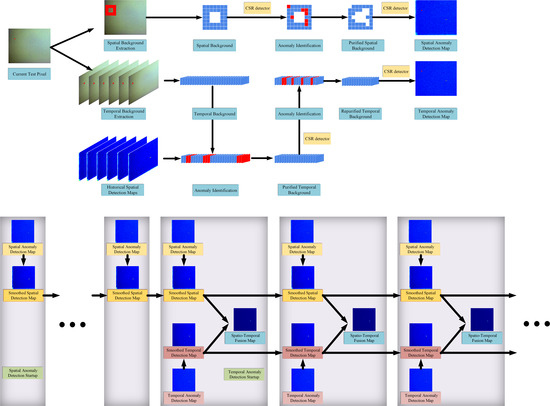
Figure 1.
The framework of the proposed CSR-ST algorithm. (a) The schematic diagram of the CSR-based spatial and temporal detectors. (b) The program flowchart of the smoothing filter and fusion on the spatial and temporal detection maps.
Figure 1.
The framework of the proposed CSR-ST algorithm. (a) The schematic diagram of the CSR-based spatial and temporal detectors. (b) The program flowchart of the smoothing filter and fusion on the spatial and temporal detection maps.

Figure 2.
False color local image around targets in the Cloud dataset. (a) Target A in the 50th frame. (b) Target A in the 500th frame. (c) Target B and Target C. (d) Target D.
Figure 2.
False color local image around targets in the Cloud dataset. (a) Target A in the 50th frame. (b) Target A in the 500th frame. (c) Target B and Target C. (d) Target D.

Figure 3.
The synthetic Terrain dataset. (a) Original false color image. (b–f) Spectral curves of background and target pixels with different noise. The blue curve is a pure target pixel; the four red curves are background pixels; orange curves are mixed target pixels with a target abundance of 40%; and green curves are mixed target pixels with a target abundance of 10%. (b) No noise. (c) SNR = 20 dB. (d) SNR = 10 dB. (e) SNR = 5 dB. (f) SNR = 0 dB.

Figure 4.
Histogram of the number of frames that targets take to pass through a single pixel in the Cloud dataset.
Figure 4.
Histogram of the number of frames that targets take to pass through a single pixel in the Cloud dataset.

Figure 5.
The fitted variation curves of AUC with time in the 101st–500th frames under different settings of the dual-window. (a) The curves of KCSR-S. (b) The curves of KCSR-T.
Figure 5.
The fitted variation curves of AUC with time in the 101st–500th frames under different settings of the dual-window. (a) The curves of KCSR-S. (b) The curves of KCSR-T.

Figure 6.
ROC curves obtained on the Cloud dataset. (a) Logarithmic abscissa; (b) linear abscissa.

Figure 7.
Color detection maps obtained in the 400th frame of the Cloud dataset. (a) False color image; (b) ground-truth map; (c) RX; (d) QLRX; (e) KRX; (f) KSVDD; (g) CR; (h) KCR; (i) CSR; (j) KCSR-S; (k) KCSR-VF; (l) KCSR-STH; (m) KCSR-SF; (n) KCSR-T; (o) KCSR-ST.
Figure 7.
Color detection maps obtained in the 400th frame of the Cloud dataset. (a) False color image; (b) ground-truth map; (c) RX; (d) QLRX; (e) KRX; (f) KSVDD; (g) CR; (h) KCR; (i) CSR; (j) KCSR-S; (k) KCSR-VF; (l) KCSR-STH; (m) KCSR-SF; (n) KCSR-T; (o) KCSR-ST.

Figure 8.
ROC curves obtained on the synthetic Terrain dataset. (a,b) adopt logarithmic abscissas and (c,d) adopt linear abscissas. (a) SNR = 20 dB; (b) SNR = 10 dB; (c) SNR = 5 dB; (d) SNR = 0 dB.
Figure 8.
ROC curves obtained on the synthetic Terrain dataset. (a,b) adopt logarithmic abscissas and (c,d) adopt linear abscissas. (a) SNR = 20 dB; (b) SNR = 10 dB; (c) SNR = 5 dB; (d) SNR = 0 dB.

Figure 9.
Color detection maps obtained in the 60th frame of the synthetic Terrain dataset when SNR = 20 dB. (a) False color image; (b) ground-truth map; (c) RX; (d) QLRX; (e) KRX; (f) KSVDD; (g) CR; (h) KCR; (i) CSR; (j) KCSR-S; (k) KCSR-VF; (l) KCSR-STH; (m) KCSR-SF; (n) KCSR-T; (o) KCSR-ST.
Figure 9.
Color detection maps obtained in the 60th frame of the synthetic Terrain dataset when SNR = 20 dB. (a) False color image; (b) ground-truth map; (c) RX; (d) QLRX; (e) KRX; (f) KSVDD; (g) CR; (h) KCR; (i) CSR; (j) KCSR-S; (k) KCSR-VF; (l) KCSR-STH; (m) KCSR-SF; (n) KCSR-T; (o) KCSR-ST.

Figure 10.
Color detection maps obtained in the 70th frame of the synthetic Terrain dataset when SNR = 10 dB. (a) False color image; (b) ground-truth map; (c) RX; (d) QLRX; (e) KRX; (f) KSVDD; (g) CR; (h) KCR; (i) CSR; (j) KCSR-S; (k) KCSR-VF; (l) KCSR-STH; (m) KCSR-SF; (n) KCSR-T; (o) KCSR-ST.
Figure 10.
Color detection maps obtained in the 70th frame of the synthetic Terrain dataset when SNR = 10 dB. (a) False color image; (b) ground-truth map; (c) RX; (d) QLRX; (e) KRX; (f) KSVDD; (g) CR; (h) KCR; (i) CSR; (j) KCSR-S; (k) KCSR-VF; (l) KCSR-STH; (m) KCSR-SF; (n) KCSR-T; (o) KCSR-ST.

Figure 11.
Color detection maps obtained in the 80th frame of the synthetic Terrain dataset when SNR = 5 dB. (a) False color image; (b) ground-truth map; (c) RX; (d) QLRX; (e) KRX; (f) KSVDD; (g) CR; (h) KCR; (i) CSR; (j) KCSR-S; (k) KCSR-VF; (l) KCSR-STH; (m) KCSR-SF; (n) KCSR-T; (o) KCSR-ST.
Figure 11.
Color detection maps obtained in the 80th frame of the synthetic Terrain dataset when SNR = 5 dB. (a) False color image; (b) ground-truth map; (c) RX; (d) QLRX; (e) KRX; (f) KSVDD; (g) CR; (h) KCR; (i) CSR; (j) KCSR-S; (k) KCSR-VF; (l) KCSR-STH; (m) KCSR-SF; (n) KCSR-T; (o) KCSR-ST.


Table 1.
The mean AUC performance achieved by KCSR-T on the Cloud dataset with different settings of the temporal background dictionary.
Table 1.
The mean AUC performance achieved by KCSR-T on the Cloud dataset with different settings of the temporal background dictionary.
| NC | 20 | 30 | 50 | 80 | 100 | |
|---|---|---|---|---|---|---|
| NR | ||||||
| 10 | 0.970966 | 0.978610 | 0.980203 | 0.978596 | 0.978292 | |
| 20 | - | 0.976092 | 0.980302 | 0.979089 | 0.978912 | |
| 30 | - | - | 0.97940 | 0.979447 | 0.979326 | |
| 40 | - | - | 0.978459 | 0.979405 | 0.979726 | |
Table 2.
The mean AUC performance achieved by KCSR-T on the synthetic Terrain dataset in four noise conditions with different settings of the temporal background dictionary. (a) SNR = 20 dB.
a
| NC | 20 | 30 | 40 | 50 | |
|---|---|---|---|---|---|
| NR | |||||
| 10 | 0.997661 | 0.998487 | 0.998910 | 0.999168 | |
| 20 | - | 0.998424 | 0.998939 | 0.999258 | |
| 30 | - | - | 0.998367 | 0.999095 | |
| 40 | - | - | - | 0.998408 | |
b
| NC | 20 | 30 | 40 | 50 | |
|---|---|---|---|---|---|
| NR | |||||
| 10 | 0.922512 | 0.926485 | 0.929855 | 0.931893 | |
| 20 | - | 0.925626 | 0.930665 | 0.932968 | |
| 30 | - | - | 0.926307 | 0.930971 | |
| 40 | - | - | - | 0.927911 | |
c
| NC | 20 | 30 | 40 | 50 | |
|---|---|---|---|---|---|
| NR | |||||
| 10 | 0.807302 | 0.810852 | 0.814612 | 0.816796 | |
| 20 | - | 0.811735 | 0.817965 | 0.819948 | |
| 30 | - | - | 0.814413 | 0.818968 | |
| 40 | - | - | - | 0.815303 | |
d
| NC | 20 | 30 | 40 | 50 | |
|---|---|---|---|---|---|
| NR | |||||
| 10 | 0.670573 | 0.681748 | 0.679998 | 0.682716 | |
| 20 | - | 0.678515 | 0.683091 | 0.685078 | |
| 30 | - | - | 0.681748 | 0.685298 | |
| 40 | - | - | - | 0.684125 | |
Table 3.
The mean AUC performance achieved by KCSR-S and KCSR-T on the Cloud dataset with different settings of the temporal background dictionary.
Table 3.
The mean AUC performance achieved by KCSR-S and KCSR-T on the Cloud dataset with different settings of the temporal background dictionary.
| (3, 5) | (9, 11) | (13, 15) | (19, 21) | (23, 25) | (29, 31) | |
|---|---|---|---|---|---|---|
| KCSR-S | 0.961412 | 0.969947 | 0.970367 | 0.970251 | 0.968993 | 0.964927 |
| KCSR-T | 0.980175 | 0.979962 | 0.979918 | 0.980145 | 0.980115 | 0.980010 |
Table 4.
The mean AUC performance obtained on the Cloud dataset.
| RX | QLRX | KRX | KSVDD | CR | KCR | CSR | KCSR-S | KCSR-VF | KCSR-STH | KCSR-SF | KCSR-T | KCSR-ST |
|---|---|---|---|---|---|---|---|---|---|---|---|---|
| 0.9371 | 0.9440 | 0.9644 | 0.9617 | 0.9360 | 0.9442 | 0.9620 | 0.9649 | 0.9784 | 0.9892 | 0.9901 | 0.9803 | 0.9976 |
Table 5.
The mean AUC performance obtained on the synthetic Terrain dataset.
| SNR | RX | QLRX | KRX | KSVDD | CR | KCR | CSR | KCSR-S | KCSR-VF | KCSR-STH | KCSR-SF | KCSR-T | KCSR-ST |
|---|---|---|---|---|---|---|---|---|---|---|---|---|---|
| 20 | 0.7696 | 0.8400 | 0.6407 | 0.6166 | 0.8199 | 0.8371 | 0.7889 | 0.8402 | 0.8829 | 0.8852 | 0.9228 | 0.9993 | 0.9996 |
| 10 | 0.7047 | 0.6778 | 0.6204 | 0.6128 | 0.7323 | 0.7438 | 0.6970 | 0.7325 | 0.7664 | 0.7769 | 0.8888 | 0.9330 | 0.9959 |
| 5 | 0.6465 | 0.6383 | 0.5881 | 0.6051 | 0.6905 | 0.7057 | 0.6591 | 0.6858 | 0.7136 | 0.7265 | 0.8162 | 0.8199 | 0.9461 |
| 0 | 0.5155 | 0.6219 | 0.4960 | 0.5705 | 0.6007 | 0.6205 | 0.5769 | 0.5943 | 0.5671 | 0.6005 | 0.6390 | 0.6851 | 0.7516 |
© 2020 by the authors. Licensee MDPI, Basel, Switzerland. This article is an open access article distributed under the terms and conditions of the Creative Commons Attribution (CC BY) license (http://creativecommons.org/licenses/by/4.0/).
Share and Cite
MDPI and ACS Style
Li, Z.; Ling, Q.; Wu, J.; Wang, Z.; Lin, Z. A Constrained Sparse-Representation-Based Spatio-Temporal Anomaly Detector for Moving Targets in Hyperspectral Imagery Sequences. Remote Sens. 2020, 12, 2783. https://doi.org/10.3390/rs12172783
AMA Style
Li Z, Ling Q, Wu J, Wang Z, Lin Z. A Constrained Sparse-Representation-Based Spatio-Temporal Anomaly Detector for Moving Targets in Hyperspectral Imagery Sequences. Remote Sensing. 2020; 12(17):2783. https://doi.org/10.3390/rs12172783
Chicago/Turabian StyleLi, Zhaoxu, Qiang Ling, Jing Wu, Zhengyan Wang, and Zaiping Lin. 2020. "A Constrained Sparse-Representation-Based Spatio-Temporal Anomaly Detector for Moving Targets in Hyperspectral Imagery Sequences" Remote Sensing 12, no. 17: 2783. https://doi.org/10.3390/rs12172783
Note that from the first issue of 2016, this journal uses article numbers instead of page numbers. See further details here.