Construction of High Spatial-Temporal Water Body Dataset in China Based on Sentinel-1 Archives and GEE


1
State Key Laboratory of Remote Sensing Science, Aerospace Information Research Institute, Chinese Academy of Sciences, Beijing 100094, China
2
School of Electronic, Electrical and Communication Engineering, University of Chinese Academy of Sciences, Beijing 100049, China
3
National Engineering Research Center for Geomatics, Aerospace Information Research Institute, Chinese Academy of Sciences, Beijing 100094, China
*
Author to whom correspondence should be addressed.
Remote Sens. 2020, 12(15), 2413; https://doi.org/10.3390/rs12152413
Submission received: 26 June 2020
/
Revised: 14 July 2020
/
Accepted: 24 July 2020
/
Published: 28 July 2020
(This article belongs to the Special Issue Remote Sensing of Wetlands)
Abstract
:Surface water is the most important resource and environmental factor in maintaining human survival and ecosystem stability; therefore, timely accurate information on dynamic surface water is urgently needed. However, the existing water datasets fall short of the current needs of the various organizations and disciplines due to the limitations of optical sensors in dynamic water mapping. The advancement of the cloud-based Google Earth Engine (GEE) platform and free-sharing Sentinel-1 imagery makes it possible to map the dynamics of a surface water body with high spatial-temporal resolution on a large scale. This study first establishes a water extraction method oriented towards Sentinel-1 Synthetic Aperture Radar (SAR) data based on the statistics of a large number of samples of land-cover types. An unprecedented high spatial-temporal water body dataset in China (HSWDC) with monthly temporal and 10-m spatial resolution using the Sentinel-1 data from 2016 to 2018 is developed in this study. The HSWDC is validated by 14,070 random samples across China. A high classification accuracy (overall accuracy = 0.93, kappa coefficient = 0.86) is achieved. The HSWDC is highly consistent with the Global Surface Water Explorer dataset and water levels from satellite altimetry. In addition to the good performance of detecting frozen water and small water bodies, the HSWDC can also classify various water cover/uses, which are obtained from its high spatial-temporal resolution. The HSWDC dataset can provide more detailed information on surface water bodies in China and has good application potential for developing high-resolution wetland maps.
1. Introduction
Surface water, as the most important terrestrial resource, is undergoing spatial and temporal changes caused by many factors, such as land-use/cover changes, climate changes, seasonal changes, and environmental changes, throughout the world [1]. Quantifying spatiotemporal dynamics of surface water resources will provide decision makers with information for feasible wetland restoration and management strategies and to further evaluate their effects [2].
Many water body databases have been developed in previous studies. The Shuttle Radar Topography Mission (SRTM) water body data is available at latitudes from 56°S to 60°N with a resolution of 30 m [3]. Verpoorter et al. [4] produced a global water body database with a 14.25-m spatial resolution. Feng et al. [5] develop the Global Land Cover Facility inland surface water dataset at a 30-m resolution for circa-2000. A global water mask based on MODIS archives is produced by Carroll et al. [1]. The aforementioned studies produced static water maps and can meet some applications, but the demand for information on the spatial and temporal changes of inland water bodies and their long-term evolution is still growing [6]. Therefore, many authors have already attempted to map dynamic changes of water bodies [7,8,9,10,11,12,13]. These datasets provide information on the extent of the water bodies at daily to monthly intervals and cover a limited geographic area. Pekel et al. [11] produced an excellent Global Surface Water Explorer (GSWE) dataset with 30-m spatial resolution and a monthly time interval. It comes from the entire multi-temporal orthorectified Landsat 5, 7 and 8 archive spanning the past 32 years and shows the spatial and temporal variability of global surface water and its long-term changes. However, due to the limitations of optical data, the above efforts for monitoring the water body dynamics are still in need of further improvement. For example, GSWE still cannot form regular periodic monitoring of water body dynamics. The dynamic water dataset formed by time series interpolation is also affected by the model itself.
Synthetic Aperture Radar (SAR) data have the advantage of being unaffected by clouds, so they can be used to regularly monitor surface water [14,15]. Yet, due to the difficulty of SAR data acquisition at large scale and the complexity of data processing, in the past, water body monitoring and mapping using SAR data has mainly focused on individual bodies of water or specific small areas [16,17,18]. With the free distribution of Sentinel-1 data, as well as the release and application of the Google Earth Engine (GEE) platform, it is possible to carry out dynamic monitoring and mapping of water bodies on a large scale. At the same time, Sentinel-1 provides data on 10-m resolution, which can produce more accurate water maps that include many small water bodies that are missed by the aforementioned surface water data products. Furthermore, hydrological inputs and outputs influence soil biochemistry, and characteristics of flooding such as duration, spatial extent, and timing of high and low waters drive plants’ germination and growth [19,20]. Quantifying long-term spatiotemporal hydro-period variability and changes are fundamentally important for wetland management and restoration. Therefore, it is of significance to provide the high-precision surface water dynamic information.
In order to explore the potentiality of Sentinel-1 in large-scale water body mapping and obtain an unprecedented high spatial-temporal water body dataset, in this study, our work includes: (1) establishing a large-scale water classification method based on time series Sentinel-1 data, (2) extracting China surface water body on monthly temporal and 10-m spatial resolution from 2016 to 2018 based on the GEE platform and evaluating of its accuracy, and (3) comparing our dataset with existing water products to assess their spatial and temporal differences.
2. Data Sources and Availability
Sentinel-1 is the first of the Copernicus Programme satellite constellations created by the European Space Agency. This space mission is composed of two satellites, Sentinel-1A and Sentinel-1B, carrying a C-band (~5.7 cm wavelength) SAR instrument offering data products in single (HH or VV) or double (HH + VH or VV + VH) polarization [16]. There is a total of 73,128 ground range detected (GRD) images from 2016 to 2018, covering all of mainland China (Figure 1). We determined that the observation frequency at same location ranges from 17 to 128 during 2018, which can meet the monthly water mapping of China. The auxiliary data includes Landsat Operational Land Imager (OLI) image, the SRTM DEM, and GSWE. The water level dataset, GSWE and the time series of inland surface water dataset in China (ISWDC) are used for cross comparison [9,11,21]. Table 1 summarizes all of the datasets and tools used in this paper.
3. Methods
The main technical route of this study includes four major parts (Figure 2): (1) preliminary extraction of water body based on Sentinel-1 archive, (2) acquisition of the auxiliary water mask, (3) post-processing for water extraction, and (4) accuracy validation of the high spatial-temporal water body dataset in China (HSWDC).
3.1. Preliminary Extraction of Water Body
In the first step, we first implement monthly mean composite using monthly Sentinel-1 images. The Sentinel-1 data covering China include two polarization modes: VV polarization and VH polarization. With reference to existing research, water bodies based on the two polarization modes have different thresholds [16]. In order to verify the feasibility of the threshold method, we divide land cover into seven land-cover types, referring to Copernicus Global Land Cover Layers—Collection 2 and high-resolution images of Google Earth: buildings, snow, forests, crops, sand dunes, grassland and water bodies [22]. Water bodies are further divided into freshwater lakes, saltwater lakes with high mineral content, reservoirs with complex geometry, rivers, water in high mountains, and periodically frozen water bodies. Based on Copernicus Global Land Cover Layers—Collection 2, the stratified random sampling approach is used to generate sample point locations, and then they are visually confirmed one by one based on the high-resolution images on Google Earth. Finally, there are totally 550 training sample locations for these 11 land-cover types across China. At each sample location, the backscatter coefficient set of the above land-cover type are extracted based on time series Sentinel-1 VH/VV polarized images. We select 6866 backscatter coefficient samples from VH images in 2018, 6820 backscatter coefficient samples from VV images in 2017 and then calculate the median, mean, upper and lower quartiles, and 1.5 interquartile range (IQR) of these backscatter coefficients (Figure 3). The results show that all of the water body subtypes have similar values and all of the non-water land-cover types, except for sand dunes, have good separability with water bodies. With all this, on the VV polarization image, the pixels with a backscattering coefficient value not greater than −15 dB are regarded as a body of water, and on the VH polarization image, the pixels with a backscattering coefficient value not greater than −23 dB are regarded as a body of water. These characteristics of water bodies are what past research studies have used [16,23,24,25,26]. These characteristics also allow us to detect water bodies with periodically frozen ice in winter using the above thresholds. When using GEE and Sentinel-1 archives, this effective approach is clearly operational and efficient for large-scale water mapping.
3.2. Development of Different Water Masks
The defects of this approach are the confusion between the sand dunes, snow, terrain shadows, and waters. Therefore, we build three kinds of water masks, i.e., Water Mask-slope, Water Mask-OLI, and Max Water-GSWE, to refine the preliminary water body results produced in the first step.
Some studies have shown that synthetic ascending and descending SAR scenes reduce some errors caused by radar shadows or layover, but do not completely eliminate them [17]. Using optical sensors to detect surface water will also encounter the problem of terrain shadows, and there has been a lot of research performed using slope dataset to solve this problem [6,11,27,28]. We obtain the slope dataset from SRTM DEM by calculating the maximum elevation change rate of each grid cell to its eight neighboring cells. Finally, we use a threshold of to 3 degrees to exclude steep locations where water is unlikely to exist. We extract the pixels that have slopes less than 3 degrees from the slope dataset as Water Mask-slope.
Second, the limitation of the threshold method itself will confuse the extracted water body based on Sentinel-1 with the sand dunes dominated by dry sand. The normalized differential water body index (NDWI) can be used to distinguish between sand dunes and water; therefore, we use NDWI calculated based on Landsat OLI images to generate Water Mask-OLI. Every Landsat OLI scene during one year excludes cloud pixels by using its own quality control band, and then uses a mean composite method to obtain an annual cloudless Landsat OLI image. Each pixel value of the annual cloudless Landsat OLI image is derived from the average value of the original clean pixels. McFeeters et al. propose different NDWI calculation methods [29,30,31]. We compare these calculation methods through experiments. The results show that the calculation method developed by McFeeters et al. can best reflect the water body based on the Landsat OLI image. Since it is not the main purpose of this study, no more detailed experimental results are given in the article. With all this, the NDWI mentioned in this article is calculated using the near-infrared spectrum (0.85–0.88 μm) and the green spectrum (0.53–0.59 μm) of the annual cloudless Landsat OLI image. We use the water sample in Section 3.1 to determine that the NDWI threshold is −0.06, that is, pixels with an NDWI value greater than −0.06 are identified as a water body, and pixels with an NDWI value not greater than −0.06 are identified as a non-water body.
The water mask obtained in this way contains snow pixels. It has been proven in a previous study that the reflectivity of snow in the near infrared band is higher than that of water bodies [32]. This feature can help us exclude snow pixels in the above water mask; therefore, based on the near-infrared spectrum of the annual cloudless Landsat OLI image, the snow cover threshold (0.17) is obtained using the snow cover sample in Section 3.1. Those pixels with an NDWI value of greater than −0.06 and a near-infrared surface reflectance value of greater than 0.17 are removed from the above water mask. In order to avoid the restriction of a static mask, the annual water mask is buffered 10 m outwards to obtain Water Mask-OLI, using a morphological dilation operation [33,34].
In a study by Pekel et al. [11], the GSWE included global surface water dynamics from 1984 to 2015 in 2016, and the GSWE was later updated to 2018. The max extent water surface mask of GSWE contains any region where water has ever been detected during 1984–2018, and the max extent water surface is much larger the primary water body extraction in the first step. We use this max extent water surface as Max Water-GSWE. We resample all of these auxiliary masks to 10 m.
3.3. Post-Processing Preliminary Water Extraction
In checking the classification results by visual inspection, we find the confusion of the sand dunes and waters mainly occurs in the west region of China. So, we divide the whole of China into two parts: the east (including Beijing, Tianjin, Hebei, Liaoning, Shanghai, Zhejiang, Fujian, Shandong, Guangdong, Taiwan, Henan, Jiangsu, Anhui, Hubei, Hunan, Jiangxi and Hainan) and the west (the other provinces) (Figure 1). These commissions will be corrected using Water Mask-slope and Water Mask-OLI for the west. That is, we overlay the Water Mask-slope, Water Mask-OLI, and the primary monthly water body extracted in the first step. The pixels where the three layers are identified as the water body are the ultimate water map for the west.
There is also misclassification of water bodies with topography shadows in the east. The Max Water-GSWE is overlapped with the primary water extraction in the first step. The pixels where both layers marked as a water body are considered as ultimate water map for the east. Finally, we produce the monthly China water map by mosaicking the east water map and the west water map.
4. Results
4.1. Validation of the High Spatial-Temporal Water Body Dataset in China (HSWDC)
Pekel et al. [11] published their paper and the GSWE, which included global surface water dynamics from 1984 to 2015 in 2016, and later updated the GSWE to 2018. Based on GSWE monthly water products in 2018, we divide China into two layers of water and land, and then use the stratified random sampling method to generate a set of points on each month of GSWE products. This set of sample points, marked with the corresponding month, includes water sample points and land sample points. We firstly generate a total of 14,523 sample points from the 12-month GSWE monthly water products. Because the GSWE data itself has some misclassification errors, which mainly come from mountain shadows, saline-alkali land, ridges, and roofs (Figure 4a), we visually check those samples one by one, combining the high-resolution images from Google Earth, and remove the sample points that are clearly not water bodies. In the end, there are 14,070 samples left, including 6554 water samples and 7516 land samples (Figure 4b). In order to avoid estimation errors caused by temporal inconsistence, the verification of the HSWDC is implemented monthly using the verification samples having the same date. In this way, we can obtain the number of correctly classified and incorrectly classified water/land samples per month. The confusion matrix is finally calculated based on the sum of the above corresponding samples across the year 2018. The overall accuracy of the HSWDC is 0.93, the kappa coefficient is 0.86, the omission error is 0.14, and the commission error is 0.01.
4.2. The Temporal Dynamics of Surface Water in China
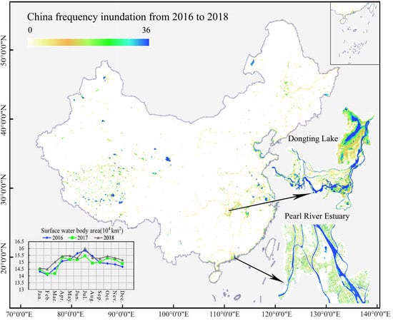
Based on the HSWDC, the maximum inundated area for the whole China in 2016, 2017, and 2018 are , and , respectively, and the minimum inundated areas are , and (Figure 5a). By comparison, Lu et al. (2018) calculate that the largest inland water area of China in 2016 is approximately , which is less than that in the HSWDC, mainly because the small water body can be identified in the HSWDC. Yet, both of them have the largest water surface area in July and the smallest in February, showing the same seasonality of China surface water.
Additionally, the spatial distributions of surface water can clearly be depicted according to average water area which is calculated from the max and min water body area in 2018 (Figure 5b). The results show that China surface water is mainly distributed in the Continental basin and Yangtze River basin, accounting for 34.94% and 26% of the total surface water area, respectively. With 8.97% in the Huaihe River basin and 8.68% in the Songhua and Liaohe River basin, followed by the Pearl River basin, which accounts for 6.25%. The Yellow River Basin, Southwest Basin, Haihe River Basin, and Southeast Basin account for the other 15.16% of the national surface water area. Furthermore, the water area of the Continental Basin, Songhua and Liaohe River Basin, Yellow River Basin, Southwest Basin, and Haihe River Basin show an increasing trend, while the other river basins show a decreasing trend, and the total water area increase slightly during the period from 2016 to 2018 (Figure 5).
5. Discussion
5.1. Comparisons with Existing Datasets
The GSWE dataset, which is based on the long-term Landsat TM, ETM, and OLI images, provides the global monthly surface water area from 1984 to 2018. However, due to the impact of clouds and the long revisit period (16 days) of Landsat satellite, GSWE cannot actually provide monthly water dynamics across most areas of China, such as in the southern China where it has a subtropical humid monsoon climate and cloudy weather occurs frequently. Figure 6 shows the monthly water dynamics of Poyang Lake (which is located in southern China) in 2018 based on the GSWE dataset and the HSWDC respectively. As expected, the GSWE cannot provide the surface water maps during January, June, and December of 2018 because of the above limitations of Landsat satellites. Furthermore, we can find GSWE only extracts part of the actual water body surface in some months, such as May, September, October, and November.
Choosing GSWE in August 2018 as the standard, it can be seen that the water surfaces extracted by HSWDC and GSWE have high consistency (gray in Figure 7). However, due to the high spatial resolution of Sentinel-1, HSWDC can present more narrow rivers and small ponds (orange in Figure 7). However, the limitations of the SAR image itself will cause some water surfaces to be missed in HSWDC (blue in Figure 7). Another possible reason for the inconsistency between the two datasets may come from the different observation date of the two satellites in the same month. The more frequent observation of waters can address this issue in the future.
Taking Dongting Lake as a sample, we also analyze the temporal consistency between the HSWDC, the GSWE and lake water level from 9 January 2016 to 25 December 2018 with a 10-day temporal resolution. The water level from satellite altimetry comes from Envisat, ERS-2, Jason-1, Jason-2, TOPEX/Poseidon, and SARAL/AltiKa, and the root mean square difference between it and in situ data ranges from 4 to 36 cm [21]. Li et al. [35] also used the water level dataset to make a comparison with the water body dataset they produced. The reason why the water area detected by HSWDC is larger than GSWE is that HSWDC has a higher spatial resolution. With the decrease of water storage, the area of some small water bodies becomes smaller, so that GSWE cannot detect them. The difference between the water surface detected by HSWDC and the water surface monitored by GSWE in winter are more significant. Since the changes in water area and elevation are inconsistent, we can only compare the trends of water extent detected by HSWDC and water level in Figure 8. The HSWDC and the water level have highly consistent seasonal variation (Pearson correlation coefficient is 0.92), while the consistency between GSWE and water level is relatively poor (Pearson correlation coefficient is 0.84) (Figure 8). The results show that the HSWDC can effectively reflect the dynamics of the water body.
5.2. Open Water Wetland Classification Based on HSWDC
The short revisit period of Sentinel-1 sensor has a good advantage in open water wetland classification. For example, the inundated duration is important for many wetland-dependent animals and plants, and even the greenhouse gas sequestration and emissions of wetlands. We can use the HSWDC data (water occurrence) to further classify waters into permanent and seasonal water types, which is key to the above ecological and environmental issues. According to the classification system of Ramsar Wetland Convention, seasonal swamps show characteristics of water during the flood period during one year, mud flats are submerged during the rainy season and exposed during the dry season, and permanent water bodies are regions that always show the characteristics of the water body in a year. By referencing the above wetland definitions and Xu et al. [36], we can identify permanent water body, mudflats, seasonal marshes and rice fields in Dongting Lake by using the water occurrence information of the HSWDC (Figure 9a). Results show that the wetland classification results by water occurrence information are consistent with the classification results of Chen et al. [37]. The difference between rice fields in Figure 9a and agricultural land in Figure 9b is that the agricultural land defined by Chen et al. includes dry crop land. One challenge in wetland mapping is water dynamics; therefore, the HSWDC could be applied to future wetland mapping to improve the accuracy of wetland classifications.
5.3. Identification of Frozen Water Body
The existing water dataset products derived from the optical images could have many omissions of mapping water bodies during the icing period, which mainly results from the limitations of the optical sensors in identifying waters and ices/snows. The free water and frozen water, however, have similar scattering coefficients on the Sentinel-1 images (Figure 2). Consequently, the SAR-based water mapping can break through the limitations of optical images and map the frozen water. Taking the Selinco Lake located on the Tibetan Plateau as an example, it begins to freeze in December and does not completely freeze until the end of January, begins to ablate in March of the following year, and achieves full ablation in April [38]. As shown in Figure 10, compared with the ISWDC, the HSWDC can map the complete water surface even during the freezing months. The advantage of the SAR-based water mapping means the HSWDC can extract a more complete surface water body when it comes to China’s water bodies.
5.4. Uncertainty of This Study
This paper proposes a threshold method based on Sentinel-1 SAR imagery to develop an unprecedented high spatiotemporal resolution water body dataset. We use 14,070 samples to verify the accuracy of HSWDC. These points are mainly derived from stratified random sampling. They may not have enough points to fall on the edge of the water body and small water body, so the actual error may be higher than the error value we obtain. The error mainly comes from two aspects: the limitation of the Sentinel-1 image itself and the error of auxiliary data.
The C-band electromagnetic wave of the Sentinel-1 sensor makes the detection of open water relatively simple, with almost no signal returning to the antenna. When the water level is high or the transmission is low, the radar signal is usually attenuated, while when the water level is low relative to the vegetation, double rebound scattering may occur [16]. Some studies have tried to detect water with obvious vegetation canopy on its surface [26,39,40], but most of these studies require the relative heights of vegetation and water surface and the distribution characteristics of vegetation leaves as input parameters of the model. These parameters need to be measured in the wild, so these existing studies are basically limited to small scales. The influence of the complex scattering mechanism between vegetation and water is difficult to unify in a large region, and the water with significant vegetation canopy over its surface contributes very little to the total amount of water in China, so we ignore it in the method we design. In addition, during the radar-scanning process, the amplitude of sub-spherical waves between pixels may be repeated or attenuated, and finally the addition, subtraction, and difference generate random variables. This phenomenon is reflected as speckle noise in SAR images. For speckle noise, previous researches provide two schemes: one is to filter the Sentinel-1 image before water extraction [41], and the other is to perform a morphological operation after water extraction to remove speckle noise [33,34]. We have conducted experiments on these two methods, and the results show that while these methods reduce noise, they also eliminate some small waters in the HSWDC, such as narrow rivers (Figure 11). Therefore, we retain the original results in our study, but the post-processing could be carried on according to their specific needs.
In checking the classification results by visual inspection, we find the confusion of the sand dunes and waters mainly occurs in the west region of China. The NDWI can be used to distinguish between sand dunes and water; therefore, we use NDWI calculated based on Landsat OLI images to generate Water Mask-OLI. In order to avoid the restriction of a static mask, the annual water mask is buffered 10 m outwards to obtain Water Mask-OLI, using a morphological dilation operation. We overlap Water Mask-OLI and the water body we produce to exclude the impact of the dunes in the west. This method is based on the assumption that the dynamic change of the surface of the western water body is less than 10 m, which could bring some uncertainty to the west region. In addition, the use of STRM DEM and GSWE maximum water extent map may limit the water surface area of HSWDC or introduce their errors to HSWDC. In the future, a new classification method that does not use these auxiliary data can be developed. Sentinel-1 data in GEE is only processed through primary processing such as noise removal, calibration and geocoding. As we all know, layover and shadow will bring some errors to the extraction of water based on radar images [17]. In this study, compositing ascending and descending SAR scenes have reduced this error but do not fully eliminate it. It is also urgent to invent a suitable method for eliminating the effects of layover and shadow on radar images at a large scale.
6. Conclusions
In this study, we develop a threshold method for the large-scale SAR-based water mapping based on massive experiments with different land-cover type samples across China. The threshold-based water mapping method, which is more universal than previous studies on individual water bodies mapping, is proven to be robust and applicable across different seasons in a year. The Sentinel-1 images from 2016 to 2018 are then employed to construct the HSWDC using the cloud-based GEE platform and other auxiliary data. Compared with the existing surface water datasets, the HSWDC has the advantages of unprecedented spatial resolution (10 m) and period observation at the month scale. In addition, the HSWDC can effectively provide surface water distribution even in the freezing period. Due to the characteristics of SAR, which are not affected by clouds, the HSWDC can be an ideal alternative data source for future wetland mapping in cloudy regions.
Author Contributions
All authors have contributed substantially and uniquely to the work reported. Y.L. designs method and writes the original manuscript draft. Z.N. conceives the research and review the manuscript draft. Z.X. processes the data. X.Y. collects basic data used in this research. All authors have read and agreed to the published version of the manuscript.
Funding
This research has been supported by the Strategic Priority Research Program of the Chinese Academy of Sciences (XDA19030203), the National Key Research and Development Program of China (2017YFA0603004), and the National Natural Science Foundation of China (41971390).
Acknowledgments
We acknowledge Google Earth Engine for providing computing platform. The radar images used in this study are free Copernicus Sentinel data, which also are provided in GEE, and other data used in this study are freely available. We thank the authors and institutions who provided us with these data. We also thank those anonymous reviewers who provide valuable suggestions for the revision of this paper.
Conflicts of Interest
The authors declare that they have no known competing financial interests or personal relationships that would have influenced the outcomes reported in this paper.
Data Availability
HSWDC dataset can be obtained by contacting the corresponding author.
References
- Carroll, M.L.; Townshend, J.R.; DiMiceli, C.M.; Noojipady, P.; Sohlberg, R.A. A new global raster water mask at 250 m resolution. Int. J. Digit. Earth 2009, 2, 291–308. [Google Scholar] [CrossRef]
- Wang, X.; Xie, S.; Zhang, X.; Cheng, C.; Hao, G.; Du, J.; Zheng, D. A robust Multi-Band Water Index (MBWI) for automated extraction of surface water from Landsat 8 OLI imagery. Int. J. Appl. Earth Obs. Geoinf. 2018, 68, 73–91. [Google Scholar] [CrossRef]
- Farr, T.G.; Rosen, P.A.; Caro, E.; Crippen, R.; Duren, R.; Hensley, S.; Kobrick, M.; Paller, M.; Rodriguez, E.; Roth, L.; et al. The shuttle radar topography mission. Rev. Geophys. 2007, 45. [Google Scholar] [CrossRef] [Green Version]
- Verpoorter, C.; Kutser, T.; Seekell, D.A.; Tranvik, L.J. A global inventory of lakes based on high-resolution satellite imagery. Geophys. Res. Lett. 2015, 41, 6396–6402. [Google Scholar] [CrossRef]
- Feng, M.; Sexton, J.O.; Channan, S.; Townshend, J.R. A global, high-resolution (30-m) inland water body dataset for 2000: First results of a topographic-spectral classification algorithm. Int. J. Digit. Earth 2016, 9, 113–133. [Google Scholar] [CrossRef] [Green Version]
- Klein, I.; Gessner, U.; Dietz, A.J.; Kuenzer, C. Global WaterPack-A 250 m resolution dataset revealing the daily dynamics of global inland water bodies. Remote Sens. Environ. 2017, 198, 345–362. [Google Scholar] [CrossRef]
- Aires, F.; Miolane, L.; Prigent, C.; Pham, B.; Papa, F. A global dynamic long-term inundation extent dataset at high spatial resolution derived through downscaling of satellite observations. J. Hydrometeorol. 2017, 18, 1305–1325. [Google Scholar] [CrossRef]
- Fluet-Chouinard, E.; Lehner, B.; Rebelo, L.M.; Papa, F.; Hamilton, S.K. Development of a global inundation map at high spatial resolution from topographic downscaling of coarse-scale remote sensing data. Remote Sens. Environ. 2015, 158, 348–361. [Google Scholar] [CrossRef]
- Lu, S.; Ma, J.; Ma, X.; Tang, H.; Zhao, H.; Hasan Ali Baig, M. Time series of Inland Surface Water Dataset in China (ISWDC) for 2000–2016 derived from MODIS archives. Earth Syst. Sci. Data Discuss. 2018, 11, 1099–1108. [Google Scholar] [CrossRef] [Green Version]
- Papa, F.; Prigent, C.; Aires, F.; Jimenez, C.; Rossow, W.B.; Matthews, E. Interannual variability of surface water extent at the global scale, 1993–2004. J. Geophys. Res. 2010, 115, D12111. [Google Scholar] [CrossRef]
- Pekel, J.F.; Cottam, A.; Gorelick, N.; Belward, A.S. High-resolution mapping of global surface water and its long-term changes. Nature 2016, 540, 418–422. [Google Scholar] [CrossRef] [PubMed]
- Fujisada, H.; Urai, M.; Iwasaki, A. Technical methodology for ASTER Global Water Body Data Base. Remote Sens. 2018, 10, 1860. [Google Scholar] [CrossRef] [Green Version]
- Abrams, M.; Crippen, R.; Fujisada, H. ASTER Global Digital Elevation Model (GDEM) and ASTER Global Water Body Dataset (ASTWBD). Remote Sens. 2020, 12, 1156. [Google Scholar] [CrossRef] [Green Version]
- Aires, F.; Prigent, C.; Fluet-Chouinard, E.; Yamazaki, D.; Papa, F.; Lehner, B. Comparison of visible and multi-satellite global inundation datasets at high-spatial resolution. Remote Sens. Environ. 2018, 216, 427–441. [Google Scholar] [CrossRef] [Green Version]
- Santoro, M. Multi-temporal synthetic aperture radar metrics applied to map open water bodies. IEEE J. Sel. Top. Appl. Earth Obs. 2014, 7, 3225–3238. [Google Scholar] [CrossRef]
- Kaplan, G.; Avdan, U. Monthly analysis of wetlands dynamics using remote sensing data. ISPRS Int. Geo-Inf. 2018, 7, 411. [Google Scholar] [CrossRef] [Green Version]
- Slinski, K.M.; Hogue, T.S.; Mccray, J.E. Active-passive surface water classification: A new method for high resolution monitoring of surface water dynamics. Geophys. Res. Lett. 2019, 46, 4694–4704. [Google Scholar] [CrossRef]
- Xing, L.; Tang, X.; Wang, H.; Fan, W.; Wang, G. Monitoring monthly surface water dynamics of Dongting Lake using Sentinel-1 data at 10 m. PeerJ 2018, 6, e4992. [Google Scholar] [CrossRef]
- Alonso, A.; Muñoz-Carpena, R.; Kaplan, D. Coupling high-resolution field monitoring and MODIS for reconstructing wetland historical hydroperiod at a high temporal frequency. Remote Sens. Environ. 2020, 247, 111807–111825. [Google Scholar] [CrossRef]
- Campbell, D.; Keddy, P.A.; Broussard, M.; McFalls-Smith, T.B. Small changes in flooding have large consequences: Experimental data from ten wetland plants. Wetlands 2016, 36, 457–466. [Google Scholar] [CrossRef]
- Schwatke, C.; Dettmering, D. DAHITI—An Innovative Approach for Estimating Water Level Time Series over Inland Water using Multi-Mission Satellite Altimetry. Hydrol. Earth Syst. Sci. 2015, 19, 4345–4364. [Google Scholar] [CrossRef] [Green Version]
- Buchhorn, M.; Lesiv, M.; Tsendbazar, N.E.; Herold, M.; Bertels, L.; Smets, B. Copernicus Global Land Cover Layers-Collection 2. Remote Sens. 2020, 12, 1044. [Google Scholar] [CrossRef] [Green Version]
- Huth, J.; Gessner, U.; Klein, I.; Hervé, Y.; Lai, X.; Oppelt, N.; Kuenzer, C. Analyzing Water Dynamics Based on Sentinel-1 Time Series—A Study for Dongting Lake Wetlands in China. Remote Sens. 2020, 12, 1761. [Google Scholar] [CrossRef]
- Binh, P.D.; Catherine, P.; Filipe, A. Surface Water Monitoring within Cambodia and the Vietnamese Mekong Delta over a Year, with Sentinel-1 SAR Observations. Water 2017, 9, 366. [Google Scholar] [CrossRef] [Green Version]
- Ezzine, A.; Darragi, F.; Rajhi, H.; Ghatassi, A. Evaluation of Sentinel-1 data for flood mapping in the upstream of Sidi Salem dam (Northern Tunisia). Arab. J. Geosci. 2018, 11, 170. [Google Scholar] [CrossRef]
- Tsyganskaya, V.; Martinis, S.; Marzahn, P. Flood monitoring in vegetated areas using multitemporal Sentinel-1 data: Impact of time series features. Water 2019, 11, 1938. [Google Scholar] [CrossRef] [Green Version]
- Lu, S.L.; Jia, L.; Zhang, L.; Wei, Y.P.; Baig, M.H.A.; Zhai, Z.K.; Meng, J.H.; Li, X.S.; Zhang, G.F. Lake water surface mapping in the Tibetan Plateau using the MODIS MOD09Q1 product. Remote Sens. Lett. 2017, 8, 224–233. [Google Scholar] [CrossRef]
- Huang, S.F.; Li, J.G.; Xu, M. Water surface variations monitoring and flood hazard analysis in Dongting Lake area using long-term Terra/MODIS data time series. Nat. Hazards 2012, 62, 93–100. [Google Scholar] [CrossRef]
- McFeeters, S.K. The use of Normalized Difference Water Index (NDWI) in the delineation of open water features. Int. J. Remote Sens. 1996, 17, 1425–1432. [Google Scholar] [CrossRef]
- Gao, B. NDWI-A normalized difference water index for remote sensing of vegetation liquid water from space. Remote Sens. Environ. 1996, 58, 257–266. [Google Scholar] [CrossRef]
- Rogers, A.S.; Kearney, M.S. Reducing signature variability in unmixing coastal marsh Thematic Mapper scenes using spectral indices. Int. J. Remote Sens. 2004, 25, 2317–2335. [Google Scholar] [CrossRef]
- Liang, H.; Huang, X.D.; Wang, Y.L.; Gao, J.L.; Ma, X.F.; Liang, T.G. Analysis of thin snow spectral characteristic and retrieval algorithm construction of the fractional snow cover in Qilian Binggou Basin. Pratacult. Sci. 2017, 34, 1353–1364. [Google Scholar] [CrossRef]
- Gstaiger, V.; Huth, J.; Gebhardt, S.; Wehrmann, T.; Kuenzer, C. Multi-sensoral and automated derivation of inundated areas using TerraSAR-X and ENVISAT ASAR data. Int. J. Remote Sens. 2012, 33, 7291–7304. [Google Scholar] [CrossRef]
- Xiong, L.; Deng, R.; Li, J.; Liu, X.; Yan, Q.; Liang, Y.; Liu, Y. Subpixel surface water extraction (SSWE) Using Landsat 8 OLI Data. Water 2018, 10, 653. [Google Scholar] [CrossRef] [Green Version]
- Li, L.L.; Skidmore, A.; Vrieling, A. A new dense 18-year time series of surface water fraction estimates from MODIS for the Mediterranean region. Hydrol. Earth Syst. Sci. 2019, 23, 3037–3056. [Google Scholar] [CrossRef] [Green Version]
- Xu, X.L.; Liu, L. Cropping rotation system data of China. Acta Geol. Sin. 2014, 69, 49–53. [Google Scholar] [CrossRef]
- Chen, Y.F.; Niu, Z.G.; Hu, S.J.; Zhang, H.Y. Dynamic monitoring of Dongting Lake using time-series MODIS imagery. J. Hydraul. Eng. 2016, 47, 1093–1104. [Google Scholar] [CrossRef]
- Wang, Q.; Wang, J.B.; Guo, J.Y.; Liang, J. Lake Ice Extraction of Selin Co and its space-time distribution based on Support Vector Machine. Manned Spacefl. 2019, 25, 789–798. [Google Scholar] [CrossRef]
- Grimaldi, S.; Xu, J.; Li, Y.; Pauwels, V.R.N.; Walker, J.P. Flood mapping under vegetation using single SAR acquisitions. Remote Sens. Environ. 2020, 237, 111582–111601. [Google Scholar] [CrossRef]
- Brisco, B.; Shelat, Y.; Murnaghan, K.; Montgomery, J.; Fuss, C.; Olthof, I.; Hopkinson, C.; Deschamps, A.; Poncos, V. Evaluation of C-band SAR for identification of flooded vegetation in emergency response products. Can. J. Remote. Sens. 2019, 45, 73–87. [Google Scholar] [CrossRef]
- Fu, B.; Wang, Y.; Campbell, A.; Li, Y.; Zhang, B.; Yin, S.; Xing, Z.; Jin, X. Comparison of object-based and pixel-based Random Forest algorithm for wetland vegetation mapping using high spatial resolution GF-1 and SAR data. Ecol. Indic. 2017, 73, 105–117. [Google Scholar] [CrossRef]
Figure 1.
(a) Spatial distribution of Sentinel-1 observations in 2018 and (b) the number of images per month used for 2016, 2017, and 2018. The boundary layer of China is from National Administration of Surveying, Mapping, and Geoinformation of China: GS (2016)1569.
Figure 1.
(a) Spatial distribution of Sentinel-1 observations in 2018 and (b) the number of images per month used for 2016, 2017, and 2018. The boundary layer of China is from National Administration of Surveying, Mapping, and Geoinformation of China: GS (2016)1569.

Figure 2.
Flow diagram of this study.

Figure 3.
The backscatter coefficients of 11 land-cover types on (a) VH polarized images and (b) VV polarized images.
Figure 3.
The backscatter coefficients of 11 land-cover types on (a) VH polarized images and (b) VV polarized images.

Figure 4.
(a) Some error sample points from the GSWE water product ((a1) mountain shadow, (a2) saline-alkali land, (a3) ridge and (a4) roof); (b) China geographic distribution of water samples points. (China boundary layer is from National Administration of Surveying, Mapping, and Geoinformation of China: GS (2016)1569).

Figure 5.
(a) Monthly changes in China water area during the period of 2016–2018, (b) the max and min surface water body area () of each basin during 2016–2018. The boundary of basins comes from the Institute of Geographical Sciences and Natural Resources Research, Chinese Academy of Sciences.
Figure 5.
(a) Monthly changes in China water area during the period of 2016–2018, (b) the max and min surface water body area () of each basin during 2016–2018. The boundary of basins comes from the Institute of Geographical Sciences and Natural Resources Research, Chinese Academy of Sciences.

Figure 6.
Comparison of monthly water dynamics of Poyang Lake during 2018 based on the GSWE dataset (blue) and the HSWDC dataset (red).
Figure 6.
Comparison of monthly water dynamics of Poyang Lake during 2018 based on the GSWE dataset (blue) and the HSWDC dataset (red).

Figure 7.
Comparison of Poyang Lake in August 2018 from the HSWDC and the GSWE. The region where both HSWDC and GSWE are recognized as water is shown in grey. Based on GSWE, the over-extracted water surface of HSWDC is shown in orange, and the under-extracted water surface of HSWDC is shown in blue. (a,b) are two local regions of Poyang Lake.

Figure 8.
A comparison of time series of the surface water extent derived from HSWDC (shown in orange), GSWE (shown in gray), and water level from satellite altimetry (shown in blue) during 2016 to 2018.
Figure 8.
A comparison of time series of the surface water extent derived from HSWDC (shown in orange), GSWE (shown in gray), and water level from satellite altimetry (shown in blue) during 2016 to 2018.

Figure 9.
(a) Wetland classification of Dongting Lake based on water occurrences of the HSWDC. (The number of flooding 1 is defined as rice fields, 2–4 as seasonal marshes, 5–11 as mudflats, and 12 as permanent waters during one year). (b) Classification results of Dongting Lake from Chen et al. (2016).

Figure 10.
The map of Selinco Lake and small water body in January 2016 in (a) inland surface water dataset in China (ISWDC) and (b) high spatial-temporal water body dataset in China (HSWDC).
Figure 10.
The map of Selinco Lake and small water body in January 2016 in (a) inland surface water dataset in China (ISWDC) and (b) high spatial-temporal water body dataset in China (HSWDC).

Figure 11.
(a) Result obtained by the Refined Lee filter before water body extraction, (b) result of original image, (c) result obtained by morphological operators (first erosion, then dilation) after water body extraction.
Figure 11.
(a) Result obtained by the Refined Lee filter before water body extraction, (b) result of original image, (c) result obtained by morphological operators (first erosion, then dilation) after water body extraction.


Table 1.
All datasets and tools used in this study.
| Data/Product Name | Spatial Resolution | Temporal Resolution | Purpose in the Study | Download Link |
|---|---|---|---|---|
| Sentinel-1 ground range detected (GRD) products | 10 m | 6-d | Generate time series of water fraction maps | https://scihub.copernicus.eu/dhus/#/home |
| Landsat operational land imager(OLI) images in 2018 | 30 m | 16-d | Eliminate the effects of western terrain shadows and deserts | https://doi.org/10.5066/F78S4MZJ |
| Digital elevation model from Shuttle Radar Topography Mission (SRTM) | 30 m | static | Identification of sloping terrain and terrain shadows | https://doi.org/10.5066/F7PR7TFT |
| Global Surface Water Explorer (GSWE) maximum water extent map during 1984 to 2018 | 30 m | static | Eliminate the effects of western mountains | https://global-surface-water.appspot.com/download |
| GSWE monthly water history in 2018 | 30 m | monthly | To generate threshold estimation points and validation points, comparison of products | https://global-surface-water.appspot.com/download |
| Water level from satellite altimetry | 10-d | Comparison of products | https://dahiti.dgfi.tum.de/en/ | |
| Copernicus Global Land Cover Layers—Collection 2 | 100 m | static | As a reference for the selection of threshold samples and landcover types | https://doi.org/10.5281/zenodo.3243509 |
| Inland surface water dataset in China (ISWDC) | 500 m | 8-d | Comparison of products | http://doi.org/10.5281/zenodo.1463694 |
| Standard China map | Define a correct boundary of China | http://bzdt.ch.mnr.gov.cn/ | ||
| Boundary of basins | Define a boundary of basins | http://www.resdc.cn/data.aspx?DATAID=141 | ||
| Google Earth Engine | Provide computing resources | https://earthengine.google.com |
© 2020 by the authors. Licensee MDPI, Basel, Switzerland. This article is an open access article distributed under the terms and conditions of the Creative Commons Attribution (CC BY) license (http://creativecommons.org/licenses/by/4.0/).
Share and Cite
MDPI and ACS Style
Li, Y.; Niu, Z.; Xu, Z.; Yan, X. Construction of High Spatial-Temporal Water Body Dataset in China Based on Sentinel-1 Archives and GEE. Remote Sens. 2020, 12, 2413. https://doi.org/10.3390/rs12152413
AMA Style
Li Y, Niu Z, Xu Z, Yan X. Construction of High Spatial-Temporal Water Body Dataset in China Based on Sentinel-1 Archives and GEE. Remote Sensing. 2020; 12(15):2413. https://doi.org/10.3390/rs12152413
Chicago/Turabian StyleLi, Yang, Zhenguo Niu, Zeyu Xu, and Xin Yan. 2020. "Construction of High Spatial-Temporal Water Body Dataset in China Based on Sentinel-1 Archives and GEE" Remote Sensing 12, no. 15: 2413. https://doi.org/10.3390/rs12152413
Note that from the first issue of 2016, this journal uses article numbers instead of page numbers. See further details here.