Identifying Hydro-Geomorphological Conditions for State Shifts from Bare Tidal Flats to Vegetated Tidal Marshes

Abstract

High-lying vegetated marshes and low-lying bare mudflats have been suggested to be two stable states in intertidal ecosystems. Being able to identify the conditions enabling the shifts between these two stable states is of great importance for ecosystem management in general and the restoration of tidal marsh ecosystems in particular. However, the number of studies investigating the conditions for state shifts from bare mudflats to vegetated marshes remains relatively low. We developed a GIS approach to identify the locations of expected shifts from bare intertidal flats to vegetated marshes along a large estuary (Western Scheldt estuary, SW Netherlands), by analyzing the interactions between spatial patterns of vegetation biomass, elevation, tidal currents, and wind waves. We analyzed false-color aerial images for locating marshes, LIDAR-based digital elevation models, and spatial model simulations of tidal currents and wind waves at the whole estuary scale (~326 km²). Our results demonstrate that: (1) Bimodality in vegetation biomass and intertidal elevation co-occur; (2) the tidal currents and wind waves change abruptly at the transitions between the low-elevation bare state and high-elevation vegetated state. These findings suggest that biogeomorphic feedback between vegetation growth, currents, waves, and sediment dynamics causes the state shifts from bare mudflats to vegetated marshes. Our findings are translated into a GIS approach (logistic regression) to identify the locations of shifts from bare to vegetated states during the studied period based on spatial patterns of elevation, current, and wave orbital velocities. This GIS approach can provide a scientific basis for the management and restoration of tidal marshes.

1. Introduction

Different stable states have been observed in many ecosystems and identified as an important constraint on ecological management and restoration [1,2,3]. Understanding the conditions under which shifts can be expected to happen from one ecosystem state to another, has been widely recognized as an important challenge. Identifying the conditions for these shifts has been found to be difficult due to several factors. First, it is difficult to know whether a system is close to a catastrophic bifurcation unless the critical transition is already happening [2,4], and secondly, once the critical shift has occurred, it may be difficult to restore the ecosystem to its original state due to hysteresis effects [2,5]. Recent studies have investigated the conditions that lead to such shifts in different ecosystems [3,6]. However, few studies aimed to identify the conditions for state shifts in biogeomorphic systems, which are governed by interactions between organisms and their geomorphologic environment.

Intertidal flats and marshes are well-known examples of biogeomorphic systems, which are shaped by interactions between vegetation establishment, flow hydrodynamics, and sediment erosion and deposition [7,8,9,10]. The significance of analyzing shifts between bare flats and vegetated marshes lies in the valuable ecosystem services provided by tidal marshes to coastal and estuarine communities [11]. They play an important role in coastal defense by mitigating storm surge flooding [12,13,14], the reduction in waves and wave-induced shoreline erosion [15,16,17], and the accretion of sediments in balance with the sea-level rise [18,19].

Increasing evidence suggests that vegetated marshes and bare flats can be considered as two stable states of intertidal ecosystems [10,20,21]. A number of studies have observed bimodality in either the distribution of vegetation biomass [10,22] or in intertidal elevation [21,23], suggesting that two stable states exist, either a stable high-lying vegetated state or a stable low-lying bare state, while intermediate elevations and biomass densities occur less frequently [10,21]. Purely physical models of feedbacks between wave erosion and water depth have been proposed to explain the stable state of the low-lying bare flat [20,24,25]. These models indicate that wave-induced erosion on a bare tidal flat is dependent on the water depth, with maximum erosion being reached at a critical intermediate water depth. Assuming a constant background sediment deposition rate, the models show that the sediment bottom accretes from a deep water bottom until a certain water depth is reached, where the wave-induced erosion balances the deposition, and a stable low-lying bare tidal flat emerges. If the water depth became shallower, wave-induced erosion would increase, hence tending to keep the tidal flat elevation in the low-lying bare stable state [20,24,25]. Biogeomorphic models, simulating feedbacks between vegetation establishment, hydrodynamic forces, and sediment deposition and erosion, have been proposed to result in the high-lying vegetated marsh state [26,27,28]. Under certain conditions, which enable the establishment of marsh plants on an initially bare tidal flat, the vegetation-induced friction will reduce the hydrodynamic forces, hence reducing erosion rates and allowing sediment accretion until a high-lying, vegetated state is reached [28,29,30]. Empirical evidence demonstrated that shifts between the bare and vegetated intertidal state can occur rather rapidly on decadal time scales when a threshold elevation is exceeded [21]. Modeling and observations have shown that such transition from a bare to vegetated intertidal state typically occur after a so-called “Window of Opportunity”, i.e., a period when favorable conditions occur that enable plant seedlings to establish [29,30]. Especially hydrodynamic conditions (periods with low frequency and duration of tidal inundation, low wave activity) have been identified as conditions for shifts from bare to vegetated intertidal states in previous studies [24,25].

Previous GIS studies on the landscape scale have mainly utilized thresholds in elevation relative to mean sea level to identify the conditions enabling shifts from bare to vegetated states [21]. In fact, elevation only indirectly affects vegetation establishment, since it lumps the effects of several variables with a more direct effect, including tidal inundation depth and duration, hydrodynamic forces from tidal currents and waves, and sediment bed dynamics [30,31,32]. These physical disturbances are potentially the main bottlenecks to new marsh establishment on tidal flats [8,33,34]. For instance, a coupled study combining numerical modeling and GIS analysis has shown that elevation only acts as a prerequisite for successful marsh seedling establishment [30]. Once a minimum elevation threshold is reached, hydrodynamic forces become the main factor determining the chance of seedling establishment.

However, on a scale of a large estuary (~10²-10³ km²), very few studies have linked the shifts from low-lying bare to high-lying vegetated states with the spatial distribution of elevation, tidal current velocity, and wave orbital velocity in intertidal ecosystems. Applying a physical model for marsh establishment at this scale, is computationally complex, as it would necessitate simulating interactions between hydrodynamics (tidal currents, waves), sediment dynamics (erosion, deposition), and vegetation dynamics (colonization, growth, die-off) at high spatial resolutions (~m²) but large domains (~10²-10³ km), and high temporal resolutions (sec) but large simulated periods (~decades). Therefore, a synthetic statistical assessment, including these factors, is expected to improve our understanding of the mechanisms that cause shifts between bare and vegetated ecosystem states and the predictability of such state shifts. The overall objective of this study is to develop the knowledge of where state shifts from the bare to vegetated state are likely to occur on a large spatial scale of an estuary (~326 km²), Western Scheldt estuary (SW Netherlands). To achieve this, a spatial statistical modeling approach that enables us to identify the locations of the shifts occurring in the intertidal zone is built. The model combines data on spatially-distributed elevation, tidal currents, and wind waves. Specifically, we use the model to address the following three questions:

(1)

Do stable states in vegetation biomass and elevation co-occur? To answer this question, we tested (1a) whether both vegetation biomass and elevation have a bimodal frequency distribution in intertidal zones; (1b) whether the spatial variation in vegetation biomass as a function of elevation shows an abrupt change from a bare to vegetated state (above a threshold elevation); and (1c) whether the temporal change in vegetation biomass is the largest in areas with an unstable intermediate elevation state;

(2)

Does hydrodynamics abruptly change between different states? We tested whether spatial variations in (2a) tidal currents and (2b) waves change abruptly between different biomass and elevation states, in order to identify potential mechanisms causing the two stable states, i.e., the biogeomorphic interactions between elevation, biomass, tidal currents, and waves;

(3)

Can we identify the location of state shifts? We examined whether we can identify the locations where shifts from bare state to vegetated state occur, based on integrating the spatially explicit data on elevation, tidal currents, and waves.

2. Materials and Methods

2.1. Study Area

The Western Scheldt, located in the southwest of the Netherlands, is the Dutch part of the Scheldt estuary, while the Belgian part of the estuary is called the Sea Scheldt (see Meire et al. [35] for more details) (Figure 1). The Western Scheldt estuary is characterized by a semi-diurnal meso- to macro-tidal regime. At spring and neap tides, the mean tidal range varied from 4.46 and 2.97 m, respectively, at the mouth, to 5.93 and 4.49 m at 91 km from the mouth. The average suspended sediment concentration (SSC) varied between 30 and 60 mg/L. The salinity in the Western Scheldt changed from 25–30 PSU (Practical Salinity Units) in the most downstream, western part of the estuary, to 5–18 PSU in the more upstream, eastern part of the estuary. As a result, from west to east, the tidal marshes ranged from salt marshes, which were dominated by halophytic plant species (including Spartina anglica, Salicornia europea, Puccinellia maritima, Halimione portulacoides, and Elymus athericus as some of the most dominant species), to brackish marshes in which both halophytic and helophytic vegetation occurred (including Scirpus maritimus, Aster tripolium, Elymus athericus, and Phragmites autralis as the dominant species). In the last 10 years, the establishment of the pioneer vegetation (largely dominated by Spartina anglica) was observed at large scales on several intertidal shoals.

2.2. Materials and Data Preprocessing

2.2.1. Aerial Images and Vegetation Maps

False-color aerial images were selected for 2 time steps (9 June 2004 and 5 July 2011) in order to study the large-scale establishment of new pioneer vegetation on intertidal shoals in between these 2 time steps. The aerial images have a scale of 1:5000 for 2004 and 1:10,000 for 2011. They were provided by Rijkswaterstaat (the Dutch governmental institute for water management) in a digitized, geo-referenced, and mosaicked format with a pixel size of 0.5 m for 2004 and 0.25 m for 2011 [36,37]. The aerial images have 3 spectral bands, that is for the near-infrared (NIR), red, and green spectra. The Normalized Difference Vegetation Index (NDVI) was used as a proxy for vegetation biomass [10,22], and was calculated from the red (R) and near-infrared (NIR) bands of the aerial images, as follows:

NDVI = (NIR − R)/(NIR + R)

(1)

Pixel values of the original aerial images were used to compute the NDVI without converting the pixel values into surface reflectance [10,22]. Pixel values of the original aerial images were linear transformations (i.e., linear rescaling) of surface reflectance values. Therefore, our NDVI values that were calculated from these pixel values were not directly comparable to the NDVI values reported in other studies, and our NDVI values calculated from the 2004 and 2011 aerial images were also not directly comparable. Nevertheless, since we have calculated NDVI using linear transforms of near-infrared and red reflectance, we considered that our NDVI values can still be used as a proxy for spatial (relative) variations in vegetation biomass within a given year (2004 or 2011), as had been done in previous remote sensing studies [10,22,38,39]. As a consequence, this analysis provided information on the relative (qualitative) spatial variations in biomass distribution rather than absolute (quantitative) biomass values.

To get a first view of the spatial distribution of biomass and elevation, we also used the vegetation maps of 2004 and 2010 from the national aerial photo surveys systematically conducted every 6 years by Rijkswaterstaat [36,40]. The vegetation maps have a horizontal accuracy of 1 m based on aerial photo interpretation with a scale of 1: 5000/1:10,000 and fieldwork. The vegetation maps distinguished between water, bare mud/sand, pioneer zone, low marsh, middle marsh, and high marsh. In this study, we reclassified these vegetation maps into bare flats (i.e., bare mud/sand, and pioneer zone in the original vegetation maps) and vegetated marshes (i.e., low, middle, and high marsh). The pioneer zones were classified as bare flats because they consisted of large areas of bare flats with only here and there very small patches of pioneer vegetation. As the analysis in this study focused on the global trends in changes from bare flats to vegetated marshes over the large estuary scale, we considered that local uncertainties in the classification would not cause significantly different results in the analysis. All the spatial analyses in this study were carried out with ArcGIS.

2.2.2. Elevation Data and Intertidal Zones

Digital Terrain Models (DTM) with a resolution of 2 × 2 m were also provided by Rijkswaterstaat. These DTMs were interpolated from LIDAR (Light Detection and Ranging) surveys performed during low tide in 2004 and 2011. Metadata on the LIDAR datasets were reported by Rijkswaterstaat as follows [37,41]. The LIDAR dataset of 2004 has a minimum vertical accuracy of 0.2 m, with the measurement point density varying from 1 point per 16 square meters to several points per square meter [41]. This means that the interpolated DTM with a resolution of 2 × 2 m contained interpolated pixel values that can be based, in some places, on several LIDAR observation points within the pixel, or in other places on LIDAR observation points that fall in nearby surrounding pixels. Interpolated DTM pixel values are, therefore, approximate, but given the very small topographic gradients that are present in the studied intertidal flat landscapes, and the resolution of the LIDAR dataset, we may assume that the vertical error on the DTM was not larger than 0.2 m, as defined for the LIDAR survey. The LIDAR dataset of 2011 had a minimum vertical accuracy of 0.1–0.15 m and a mean point density of 2 points per square meter [37]. Compared to a tidal range up to 6 m, we can consider that these error levels on the LIDAR elevations were reasonably small. For the interpolated DTM of 2011, we used the same reasoning as for the DTM of 2004, i.e., we presumed that the vertical accuracy of the DTM was within the same range of vertical accuracy as the LIDAR survey. The elevation values of the DTMs, as provided by Rijkswaterstaat, were expressed relative to the Dutch Ordnance Level (abbreviated as NAP, which was close to the mean sea level at the Dutch coast). We recalculated the DTM elevation values relative to the local mean high water level (MHWL), because this was what determined the frequency, depth, and duration of tidal inundation, and, therefore, was expected to determine the elevation limit for vegetation establishment, survival, and growth. The MHWL was calculated from tidal data recorded from 2000 to 2010 at 9 tidal gauge stations along the studied part of the estuary (see Figure 1 for locations of the tide gauge stations). The MHWL increased from 1.82 m NAP at the most seaward part of the studied estuary up to 2.98 m NAP at the most landward part, due to tidal amplification along the estuary [35]. Therefore, the MHWL surface was interpolated in between the locations of the 9 tide gauge stations. Similarly, the mean low water level (MLWL) varied along the length of the estuary, and, therefore, the MLWL surface was also interpolated from tidal data of the 9 tide gauge stations. We extracted the intertidal areas of 2004 and 2011 from the DTM as all areas above the MLWL surface. The upper boundary of the intertidal areas was formed by human land use, in particular, dikes, and was digitized visually from the aerial images.

2.2.3. Tidal Current Velocity from a TELEMAC 2D Model

High-resolution, spatially distributed tidal flow velocity data were typically not available for complex estuaries, hence tidal flow velocities in the studied estuary were simulated by a TELEMAC 2D hydrodynamic model. This model simulated depth-averaged flow velocities by solving the 2D shallow-water equations over a non-structured triangular computational mesh [42]. The implementation, calibration, and validation of a TELEMAC 2D model for the Western Scheldt estuary was described in Smolders et al. [43], and was summarized in brief below.

The computational mesh resolution increased from the downstream boundary towards the upstream boundary as the estuary narrows. For the Western Scheldt, our study area, the mesh resolution was kept constant at around 30 m. The input bathymetry of the subtidal channels was based on a Sonar survey from 2009, and the input topography of intertidal areas was based on a LIDAR survey, also from 2009; both were interpolated onto the computational mesh. At the downstream open boundary, at the mouth of the estuary, a fluctuating water level was applied to generate tides. Upstream, 7 freshwater open boundaries were implemented to introduce a daily averaged discharge to the model. Both down- and upstream boundaries used measured data from March 2009. The model was calibrated and validated using: (1) Water levels measured at 22 tidal gauge stations along the estuary (red dots in Figure 1b); (2) discharges measured (sailed ADCP) over 6 cross-sections along the estuary, i.e., Pas van Terneuzen, Everingen, Middelgat, Overloop van Hansweert, Zuidergat, and Schaar van Waarde (see red lines in Figure 1b and a close up in Figure 1c); (3) point flow velocities measured on 3 shoals, i.e., Hooge Platen with 20 locations (see location X1 in Figure 1b and a close up in Figure 1d), Rug van Baarland with 12 locations (see location X2 in Figure 1b) and Plaat van Walsoorden with 8 locations (see location X3 in Figure 1b) in the estuary. The model was calibrated stepwise by varying the bottom friction Manning’s coefficient: (1) First, it was calibrated on water levels by changing the Manning’s coefficient in between the 22 tidal gauge stations; (2) secondly, it was calibrated on total flood and ebb discharges through flood and ebb channels along the cross-sections, by varying the Manning’s coefficient between the flood and ebb channels; (3) thirdly, it was calibrated on flow velocities on the intertidal areas and eventually adapted the Manning’s coefficient locally. For more details, we refer to Smolders et al. [43,44]. For the present study, the mean tidal current velocity was extracted from the calibrated model for all points during a representative spring tide, of which the high water level was close to the yearly averaged high water level during spring tide. This mean tidal current velocity was further used in the analysis as a potential factor influencing the shifts from bare to vegetated state (see Section 2.3.3).

2.2.4. Wave Orbital Velocity from a SWAN Model

We estimated the mean of the peak near-bed orbital velocities as a potential determining factor for vegetation establishment, using the Simulating Waves Nearshore model (SWAN, [45,46,47]). The model was applied to the Western Scheldt estuary for wind conditions representative of the period 1987–2012. The model grid resolution on the intertidal areas was between 20 to 50 m (

Table 1. Model grid layout, original, rotation, extents, and grid size.

Grid	Origin		Rotation	Length		Grid Spacing
	E [m]	N [m]	[°]	x [km]	y [km]	x [km]	y [km]
0	−113,200	271,906	38.303	293	148	2.9	3
1	16,023	376,356	352.014	62.4	19.5	0.19	0.19
2	25,226	375,297	352.014	52	16.5	0.1	0.1
3	35,934	376,418	326.089	5.69	2.4	0.04	0.02
4	45,632	376,523	8.787	6.84	3.45	0.05	0.02
5	53,603	374,887	37.622	4.64	2.11	0.04	0.02
6	29,873	378,285	347.418	8.19	4.04	0.04	0.04
7	37,522	378,999	327.858	12.4	3.3	0.04	0.04
8	54,806	377,049	69.927	8.08	2.99	0.04	0.04
9	55,874	380,301	350.768	4.8	3.67	0.04	0.04
10	61,203	377,403	347.418	8.2	3.33	0.04	0.04
11	68,404	369,852	34.401	10.5	6.93	0.04	0.02

). The input bathymetry and topography were based on data from 2004. The implementation and calibration of the SWAN model for the Western Scheldt estuary was described in Callaghan et al. [48] and is shortly summarized below.

The two-dimensional SWAN wave generation and propagation model converted wind measurements into nearshore wave parameters (height, period, and direction) across the estuary. This wave model solved the oscillatory wave hydrodynamics in a parametric form using the wave action flux conservation equation. The model predictions were for wind-generated waves of periods less than 20 s. To distinguish between wind-wave velocities and tidal velocities, we considered wind-waves having a period less than 20 s, while tidal waves having a period slightly greater than 12 h. Its implementation here included the effects of wave breaking, bottom friction, wave generation, wave–wave interaction, wave shoaling, refraction, and diffraction [47,49], while wave reflection, backscatter, and vegetation induced dissipation are excluded (see Callaghan et al. [48] for more details).

The wave propagation model consisted of 12 grids. Grids ‘0’ to ‘5’ are detailed in Callaghan et al. [48]. Grid ‘1’ was extended for the present study to cover the whole Western Scheldt estuary. Further, 6 additional grids were added to this model (Table 1 and Figure 2) for this study in order to cover all intertidal areas of interest.

The model was forced by measured wind (speed and direction) and tidal water levels with a 10-min interval, ranging from 1987 to 2012 (data courtesy of Rijkswaterstaat), on 4 locations along the estuary (see Figure 2). See Callaghan et al. [48] for more details on model forcing and calibration.

The wave model provided wave height and period (spatially and temporally), which was used to estimate the near-bed peak wave orbital velocity, u_peak,bed, which was given by the following equation, assuming linear sine theory and Rayleigh distributed wave heights,

$$u_{peak,bed}^{}\approx \frac{\pi \frac{1}{1.4}{H}_{sig}}{T_p}\frac{1}{\sinh kh}$$

(2)

where $T_p$ is the peak wave period, h is the still water depth, $H_{sig}$ is the significant wave height and k is the wave number given by the linear dispersion relation of

$$kh\tanh kh=\frac{4{\pi }^2}{g{T}_p^2}h$$

(3)

where g is the gravitational acceleration. The mean of the near-bed peak wave orbital velocities was used as a potential factor for marsh vegetation establishment (Section 2.3.2 and Section 2.3.3).

2.3. Data Analysis

2.3.1. Spatial Distribution of Vegetation and Intertidal Elevation

First, we checked the frequency distribution of vegetation biomass and intertidal elevation in 2004 and 2011 to test whether bimodality occurred, which was considered as an indicator of 2 stable states. Biomass was approximated by NDVI. The frequency distribution of vegetated marshes and bare flats, which was based on the vegetation maps of 2004 and 2010, was calculated separately to check the relationship between the bimodal distribution and the presence or absence of vegetation.

Second, we analyzed the spatial variation of NDVI as a function of the elevation. A threshold elevation was hypothesized to occur, above which the biomass (NDVI) would abruptly increase from low values (representative for a bare state) to high values (representative for a densely vegetated state). We hypothesize that this threshold elevation was indicative of the unstable intermediate elevation zone. Consequently, the spatial variation of elevation was analyzed as a function of NDVI to validate the hypothesis of whether elevation abruptly changes within the NDVI range that corresponds to intermediate unstable biomass levels.

Third, we tested whether the temporal change in biomass occurs abruptly in intermediate unstable elevation zones. Hence, we calculated the change in NDVI between 2004 and 2011. The NDVI values of 2011 were first rescaled to the same scale of NDVI of 2004 using the following equation

$$NDV{I}_{2011}^{\prime }=\left(NDV{I}_{2011}-P{B}_{2011}\right)\times \frac{P{V}_{2004}-P{B}_{2004}}{P{V}_{2011}-P{B}_{2011}}+P{B}_{2004}$$

(4)

where $NDV{I}_{2011}^{\prime }$ is the new NDVI value of 2011, $NDV{I}_{2011}$ is the original NDVI value of 2011, $P{B}_{2011}$ is the NDVI value of the bare peak in 2011, $P{V}_{2011}$ is the NDVI value of the vegetated peak in 2011, $P{B}_{2004}$ is the NDVI value of the bare peak in 2004, and $P{V}_{2004}$ is the NDVI value of the vegetated peak in 2004. We analyzed the variation in the NDVI between 2004 and 2011 in relation to the elevation in 2004.

2.3.2. Spatial Variation of Currents and Waves

In order to test the hypothesis that tidal currents and wind waves change abruptly between the different states, the velocities of both currents and waves simulated, respectively, with a tidal hydrodynamic model (see Section 2.2.3) and a wave model (Section 2.2.4), were analyzed as a function of elevation and NDVI. All the parameters were combined into a raster with a resolution of 2 × 2 m using ArcGIS and were further analyzed using SPSS. The elevation and NDVI ranges that corresponded to the stable high-lying vegetated state, the stable low-lying bare state, and the unstable intermediate state were identified based on the frequency distribution of elevation and NDVI (see Section 2.3.1). Further, it was tested whether the currents and waves changed abruptly in between these states.

2.3.3. Identification of the State Shift

A multiple logistic regression model was used to identify the shift from bare flat to vegetated marshes between 2004 and 2011 based on the NDVI classification. Previous studies [30,48] have suggested that hydrodynamic variables (tidal inundation time, tidal currents, and wave-induced currents) were the key environmental variables controlling the survival and establishment of seedlings on intertidal flats. In accordance with this prior theoretical knowledge, we used the initial elevation of 2004 (as a proxy for tidal inundation time), the mean tidal current velocity during a representative spring tide in 2009, and the mean of the near-bed peak velocities in 2004 as explanatory variables in the logistic regression model. In the following analysis, the areas that were already classified as vegetated marshes in 2004 were not taken into account. The remaining areas that were bare in 2004 were subsequently classified in a dichotomous map with (1) areas that stayed bare between 2004 and 2011 and (2) areas that shifted from bare to vegetated between 2004 and 2011. We notice that inaccuracies in the classification between bare and vegetated areas may occur very locally, but as the analysis in this study focused on the global trends on the large scale of the whole estuary, we may assume that the impact of local inaccuracies on the global results were rather limited. The dichotomous map with a cell size of 0.5 m showed that zones with new marsh formation were often characterized by small-scale alterations between bare and vegetated pixels at this resolution of 0.5 m. We expected that the identification of new marsh formation at this fine resolution was very difficult based on the input environmental variables with coarser resolutions, such as 2 m for the elevation, 30 m for the tidal currents, and 20–50 m for the wave-induced currents. In addition, the time difference in this study was only 7 years (between 2004 and 2011), which means that there might not be enough time for the newly formed marsh to occupy bigger areas, even though the surrounding area had a suitable environmental condition. In order to find the most suitable spatial resolution to identify new marsh formation, we rescaled the dichotomous map with 0.5 m resolution into grids with coarser resolutions of 2 × 2, 10 × 10, 20 × 20, 30 × 30, 50 × 50, 100 × 100, and 200 × 200 m. The 100 m and 200 m resolutions were tested for an upper limit, although they might not be suitable in the end. If a certain grid contained at least 1 original pixel of new vegetation, it was defined as “new marsh”; otherwise, it was defined as “stable bare flat”. For each dichotomous classification with a different resolution (i.e., increasing grid cell size), we performed a separate logistic regression analysis, and we evaluated the model’s performance to identify the probability of the bare pixels in 2004 becoming new marsh by 2011.

Several coefficients were used to evaluate the models, such as the Nagelkerke R², correct percentage for new marshes, the correct percentage for stable bare flats, and the overall correct percentage. The threshold p-level was determined as 50%. We also assessed the accuracy of the analysis by comparing the observed percentage of new vegetation with the quantified probability. In addition, the coverage of new vegetation was mapped for the new grids to validate the analysis spatially. The new vegetation coverage was calculated as the absolute number of newly vegetated pixels in a certain grid divided by the total number of pixels in the grid.

3. Results

3.1. Spatial Distribution of Biomass and Elevation

3.1.1. Bimodality in Biomass Distribution and Elevation Distribution

The frequency distribution of NDVI at all intertidal pixels clearly indicated a bimodal distribution of vegetation biomass (Figure 3a,b). The location and range of the two peaks were consistent with the NDVI distribution of pixels that were classified as vegetated marshes and bare flats. The right peak with a broad range of positive NDVI values (e.g., between 0.1 and 0.25 in 2004) was dominated by vegetated marshes with high vegetation biomass. The left narrower peak of negative NDVI values (e.g., between −0.1 and 0 in 2004) was controlled by bare flats where vegetation was absent. The intermediate NDVI values (e.g., between 0 and 0.1 in 2004) occurred less frequently. The range and location of the NDVI distributions were different between 2004 and 2011, which could be due to two factors. First, the NDVI values were calculated from the original pixel values of the false-color aerial images, rather than the reflectance values resulting from the remote sensing images, thus, it can only provide information on the relative spatial variations in biomass distribution for a given year (2004 or 2011) rather than absolute differences in biomass distribution between years (2004 and 2011). Secondly, the images were obtained on the 9th of June 2004 and the 5th of July 2011, i.e., with a one-month difference during the growing season, hence causing potentially important differences in biomass. Nevertheless, the NDVI variation between years does not obstruct the clear observation of the bimodal distribution of biomass in the two considered years.

The elevation of all intertidal pixels also displays a bimodal distribution (Figure 3c,d). The location and range of the two peaks were in accordance with the elevation distribution of pixels that were classified as vegetated marshes and bare flats. The right narrow peak above 0 m MHWL corresponded to the high-lying vegetated marshes. The left broad peak bellow −0.4 m MHWL was attributed to the low-lying bare flats. A lack of intermediate elevations was observed between −0.4 and 0 m MHWL. Generally speaking, the curves of 2004 have shifted about 0.1 m to the right by 2011, indicating a mean sediment accumulation rate of slightly more than 0.01 m/year. The bimodal distribution in intertidal elevations can be clearly observed in 2004 and 2011.

3.1.2. Relations between Variations in Elevation and NDVI

A threshold elevation was observed, above which the spatial variation in biomass changed from a bare state to a vegetated state (Figure 4a). The NDVI of 2004 varies by around −0.05, indicating the absence of biomass, in the elevation range that was identified from Figure 3c,d as the stable, low-lying state. In the small elevation range of the intermediate, unstable state, the NDVI increased sharply to around 0.2, and then kept quasi-stable in the elevation range, which was identified as the stable, high-elevated state (Figure 4a).

Similarly, the elevation in 2004 largely varied around a mean value of about −2 m MHWL in the range of NDVI values that corresponded to the stable bare state (Figure 4b). In the intermediate unstable NDVI state, the elevation increased abruptly, to about 0 m MHWL, with increasing NDVI. In the range of NDVI values that corresponded to the stable vegetated state, the elevation was fairly constant at about 0 m MHWL, with a small variation. The variation in elevation becomes smaller with the increase in NDVI, suggesting that the increase in vegetation biomass stabilizes the elevation.

3.1.3. Abrupt Temporal Increase in Biomass in Intermediate Unstable Elevations

The biggest increase in NDVI between 2004 and 2011 was observed in the intermediate, unstable elevation range, determined according to the elevation distribution in 2004 (Figure 3c). This suggested an abrupt temporal increase in biomass in these intermediate unstable elevations (Figure 5). In the stable, high-elevated zone, the NDVI changes varied largely around a mean value that was slightly larger than zero, which may result from the fact that the aerial images were obtained earlier in the growing season, in 2004 rather than in 2011. In the stable, low-elevated zones, the NDVI changes varied slightly, at around 0, implying that there was no establishment of vegetation on these bare flats.

3.2. Spatial Variation of Hydrodynamics in between the Different States

3.2.1. Variation of Tidal Current and Wave Orbital Velocity in Relation with NDVI

Generally, the tidal current velocity declined with an increase in the NDVI value (Figure 6a). In the NDVI range corresponding to the stable bare state, the tidal current velocity gradually decreased from a mean value of 0.3 m/s to 0.1 m/s. Then, the decreasing rate slowed down by about 90% in the intermediate, unstable state and the stable, vegetated state. In the stable, vegetated state, the tidal current velocity stabilized to a value below 0.1 m/s, suggesting that the vegetation occurs in intertidal areas with a mean spring tidal current velocity below 0.1 m/s.

The wave orbital velocity generally decreases with increasing NDVI (Figure 6b). In the stable bare state, the mean value of wave velocity declined abruptly from 0.04 to 0.01 m/s. The decreasing rate slowed down by about 80% in the intermediate, unstable state, and then stabilized at close to 0 m/s in the stable, vegetated state. This suggests that vegetation occurs in intertidal areas with very low wave orbital velocities. The wave orbital velocity is about 10% of the tidal current velocity, suggesting that the Western Scheldt estuary is a tidal current-dominated system.

3.2.2. Variation of Tidal Current and Wave Orbital Velocity in Relation with Elevation

The tidal current velocity generally decreases with increasing elevation (Figure 7a). In the stable low-elevated state, the mean value declined slowly from around 0.3 to below 0.2 m/s. Once reaching the intermediate, unstable state, the rate of reduction suddenly rose about eight times faster. Finally, the rate of decrease slowed down again in the stable, high-elevated state, with flow velocities below 0.1 m/s.

The relation between the mean values of wave orbital velocity and elevation describes an arc curve that peaks within the elevation range that corresponds to the stable low-lying state (Figure 7b). The wave orbital velocity varies between 0.02 and 0.05 m/s in the stable low-lying state. It decreases sharply, to nearly 0 m/s, in the intermediate, unstable state, and stays close to 0 m/s in the stable, high-elevated state.

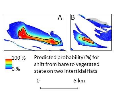
3.3. Identification of State Shift

The logistic regression, in order to identify locations (pixels) where bare flats either stay bare or shift to new marsh vegetation between 2004 and 2011, performs differently depending on the spatial resolution of the pixels (Figure 8a). With increasing pixel size, lower values were obtained for the Nagelkerke R², the overall percentage of correctly identified pixels, and the percentage of correctly identified pixels that stay bare. In contrast, the percentage of correctly identified pixels that shift to new marsh vegetation increases with increasing pixel size, i.e., a reduction in spatial resolution. The correct percentage for new marshes rises rapidly, from 30% to 50% when the pixel size increases from 2 to 30 m. With a further increase in pixel size, the increase in the correct percentage slows down. See below for further details on the logistic regression of the 30 m resolution data.

In total, seven logistic regression models were tested to identify the occurrence of new marshes using three variables, i.e., elevation, tidal current velocity, and wave orbital velocity (

Table 2. Logistic regression models identifying the shift from bare to vegetated state as a function of elevation, tidal current velocity, and wave orbital velocity, with evaluating coefficients.

No.	Parameters	Equations	Nagelkerke R2	Overall Correct Percentage	Correct Percentage for New Marshes	Correct Percentage for Stable Bare Flats
1	Elevation (E)	$\mathrm{P}=\frac{{\mathrm{e}}^{0.603+1.4\times \mathrm{E}}}{1+{\mathrm{e}}^{0.603+1.4\times \mathrm{E}}}$	0.304	85.4	22.4	97.7
2	Current velocity (C)	$\mathrm{P}=\frac{{\mathrm{e}}^{2.080-18\times \mathrm{C}}}{1+{\mathrm{e}}^{2.080-18\times \mathrm{C}}}$	0.320	84.2	23.1	96.1
3	Wave velocity (W)	$\mathrm{P}=\frac{{\mathrm{e}}^{0.304-60\times \mathrm{W}}}{1+{\mathrm{e}}^{0.304-60\times \mathrm{W}}}$	0.168	84.7	11.2	99.1
4	Elevation, current velocity	$\mathrm{P}=\frac{{\mathrm{e}}^{3.032+1\times \mathrm{E}-15\times \mathrm{C}}}{1+{\mathrm{e}}^{3.032+1\times \mathrm{E}-15\times \mathrm{C}}}$	0.435	88.8	47.3	96.9
5	Elevation, wave velocity	$\mathrm{P}=\frac{{\mathrm{e}}^{1.722+1.1\times \mathrm{E}-50\times \mathrm{W}}}{1+{\mathrm{e}}^{1.722+1.1\times \mathrm{E}-50\times \mathrm{W}}}$	0.359	86.1	34.5	96.2
6	Current velocity, wave velocity	$\mathrm{P}=\frac{{\mathrm{e}}^{3.739-17\times \mathrm{C}-60\times \mathrm{W}}}{1+{\mathrm{e}}^{3.739-17\times \mathrm{C}-60\times \mathrm{W}}}$	0.412	87.1	38.4	96.6
7	Elevation, current velocity, wave velocity	$\mathrm{P}=\frac{{\mathrm{e}}^{4.055+0.8\times \mathrm{E}-14\times \mathrm{C}-40\times \mathrm{W}}}{1+{\mathrm{e}}^{4.055+0.8\times \mathrm{E}-14\times \mathrm{C}-40\times \mathrm{W}}}$	0.475	89.0	50.1	96.6

). All of them were highly significant (p < 0.0001). Tidal current velocity was the single most explanatory variable (Model 2; Nagelkerke R² = 0.320), with slightly better performance than elevation (Model 1; Nagelkerke R² = 0.304) and much better performance than wave orbital velocity (Model 3; Nagelkerke R² = 0.168). The Nagelkerke R² increased considerably when including both elevation and tidal current velocity in the model (Model 4; Nagelkerke R² = 0.435). Adding wave velocity to the model further raised the Nagelkerke R² value to 0.475 (Model 7). The overall percentage of correctly identified pixels varied between 84% and 89%. The percentage of correctly identified stable bare pixels varied between 96% and 99%. The percentage of correctly identified new marsh pixels increased from 23% to 50% when using more explanatory variables.

The probability map (Figure 8b) for a shift from a bare to vegetated state was made by mapping the p values based on the logistic regression model. The observed map of shifts from a bare to vegetated state (Figure 8c) was made by mapping the observed percentage of new marsh pixels (with an original pixel size of 0.5 × 0.5 m) per window of 30 × 30 m, which is the resolution by which the p values are quantified with the logistic regression model. The probability map of becoming vegetated based on the Logistic Regression Model No. 7 appears fairly consistent with the observed coverage of new marshes established between 2004 and 2011 (Figure 8b,c). Large-scale establishment of new vegetation was identified on the shoals of Hooge Platen and Walsoorden, surrounded by a probability contour line of 50% (Figure 8b). The observed percentage map of the new marsh area (Figure 8c) largely coincides with the probability map (Figure 8b). The observed percentage of new marsh areas between 2004 and 2011 agrees well with the probability of new marsh areas based on the Logistic Regression Model No. 7, which was suggested by the slope of 0.95 in Figure 8d.

4. Discussion

4.1. Do Stable States in Vegetation Biomass and Elevation Co-Occur?

This work presents three pieces of evidence for the co-occurrence of stable states in vegetation biomass and elevation. Firstly, there is bimodality in the distribution of both vegetation biomass and intertidal elevations (Figure 3). Secondly, both the spatial variation in vegetation biomass as a function of elevation (Figure 4a) and the spatial variation in elevation as a function of biomass (Figure 4b), show an abrupt increase, transitioning from a stable bare, low-lying state to a stable vegetated, high-lying state, which occurs above the zone of intermediate, unstable elevations, and biomass values. Thirdly, the rate of temporal change in vegetation biomass is the highest in locations with unstable intermediate elevations (Figure 5). Further, tidal currents and waves change distinctively at the transitions between stable states in vegetation biomass and elevation, suggesting that biogeomorphic feedbacks between plant growth, flow reduction, and sedimentation are causing the shift between stable states (Figure 6 and Figure 7). Finally, this paper provides a GIS approach identifying the shift from bare to vegetated state utilizing a logistic regression model based on elevation, tidal current velocity, and wave orbital velocity as explanatory variables (Figure 8).

An important indicator of the existence of different stable states is the bimodal distribution of key variables, indicating alternative attractors [5]. Previous studies have shown that a bimodal distribution of NDVI (as a proxy of vegetation biomass) occurred at the small scale of vegetation patches in a salt marsh pioneer zone [22,50]. Other studies have shown that the elevation in intertidal zones also has a bimodal distribution [20,21,23]. Here, we show that the bimodal distribution of vegetation biomass and elevation co-occurs, indicating the existence of two stable states in the intertidal zone, i.e., either high-lying marshes with high biomass or low-lying flats with no biomass. The areas with intermediate elevation and intermediate biomass occur less frequently, suggesting that this intermediate state would be unstable and, therefore, less common.

A threshold elevation for the establishment of marsh vegetation is suggested at an elevation of about −0.4 m MHWL in the study area (Figure 4a). The threshold behavior can be explained by the associated variation in disturbance caused by tidal flooding on seedling survival [31,51]. Below the threshold elevation, it is difficult for the seedlings to survive, due to the stronger disturbance caused by tidal currents and wind waves (Figure 7), as well as by the longer, deeper, and more frequent inundation [52,53,54,55]. Above the threshold elevation, the seedlings have a higher chance of survival and establishment because of the decrease in disturbance by tidal and wind-driven currents, and tidal inundation (Figure 7) [21,51,56,57]. Once the plants manage to establish, development takes place to a high-elevation, vegetated state, characterized by low current and wave velocities (Figure 5, Figure 6 and Figure 7). This suggests the occurrence of a feedback mechanism between elevation, currents, sedimentation, and vegetation growth in causing the shift from the low-elevation bare state to the high-elevation vegetated state.

Complementing previous studies, our study demonstrates that biomass increases in the intermediate unstable state (Figure 5), suggesting the transition from bare flats to vegetated marshes. Elevation in the intermediate unstable state has also been observed to increase faster than in the stable bare state and the stable vegetated state [21]. The rapid increase in biomass and elevation in the intermediate unstable state can also be explained by positive feedbacks (suggested in Figure 6 and Figure 7) [58,59,60,61].

4.2. Does Hydrodynamics Abruptly Change between Different States?

The variation in current and wave velocities in relation to NDVI (Figure 6) and elevation (Figure 7) suggests the existence of positive feedbacks between plant growth, sedimentation, and hydrodynamic forces, resulting in two stable states [21,22,59]. When vegetation is absent on the tidal flat, the elevation varies in a critical low range of values (Figure 4b) due to the balance between sediment deposition and resuspension, which is controlled by the strong currents and waves (Figure 6) [20,25]. Marsh vegetation occurs in areas where the quantified lower values of tidal currents and wind waves (Figure 6), promoting the deposition of suspended sediment and, therefore, a rapid growth in elevation (Figure 4b) [62,63], which in turn promotes plant growth [60,64,65]. Besides, the growth of vegetation contributes to the reduction in hydrodynamic forces and, therefore, also reduces sediment erosion [61,66] (Figure 4b). Once the system reaches MHWL, the associated reduction in the inundation time would limit the further increase in elevation, thus the system becomes stable with an elevation slightly above MHWL and with more biomass (Figure 4b) [7,62,63].

The variation in tidal current velocity and wave orbital velocity as a function of elevation (Figure 7) is in agreement with earlier studies [30]. The nearly negative linear correlation between average tidal current velocity and elevation in the stable bare state (Figure 7a) is analogous to the results calculated with a two-dimensional finite element model [23,25]. The arc-shaped curve (Figure 7b) of the relation between wave orbital velocity and elevation (with a peak at intermediate elevations) is qualitatively in agreement with the conceptual model of wave generation in shallow water [20,24]. According to the model, the bottom shear stresses produced by wind waves is a function of water depth, with the maximum at a critical intermediate water depth [20]. The bottom shear stress is limited in shallow water due to dissipative processes such as bottom friction and breaking. On the other hand, the bottom shear stress is also limited in deep water, because the bottom is too deep to be influenced by the wave motions. The critical intermediate elevation was computed to be around the mean low water level by a two-dimensional wind-wave–tidal current model of the Venice lagoon [24]. Similarly, the peak of bottom wave velocity is located at around the mean low water level (between −4 and −3 m MHWL) in our study. In contrast to the study on the Venice lagoon [24], the bottom wave velocity in our study shows high values within a broader range of elevation (between −4 and −1.5 m MHWL), probably due to the much larger tidal range (up to 5 m). The tidal range in the Venice lagoon is only between 1 and 1.5 m, and consequently, tidal flats are concentrated in a narrower elevation range. As the tidal range decreases, the range of elevations affected by wave erosion decreases [67].

4.3. Can We Predict the Location of State Shifts?

Elevation has been recognized to be the bulk variable determining the appearance of new marshes and their subsequent stability, compared to other factors such as soil drainage, waves, tidal prism, and tidal range [68,69]. Other variables, such as tidal currents and waves, are much less considered in the prediction of new marsh formation on the large scale of whole estuaries or coastal lagoons [30], although small-scale experimental studies on the scale of individual pioneer plants have demonstrated the importance of hydrodynamic disturbance for pioneer plant survival and establishment (e.g., [53,70]). In this study, we included not only the elevation, but also the tidal current velocity and wave orbital velocity in the analysis of new marsh formation at the large scale of an estuary. According to the logistic regression analyses, the usage of more explanatory variables significantly improved the performance of the model (Table 2). As expected, tidal current velocity is an important explanatory variable in such a current-dominated, macro-tidal system. Overall, we have provided a successful case of spatially identifying the shift from bare to vegetated state in intertidal ecosystems at the large scale of a whole estuary, based on multiple logistic regression analysis coupled with spatial data on elevation, and spatial model simulations of tidal current and wave orbital velocities. Logistic regression has recently been broadly used to identify the transitions between stable states in different ecosystems, such as the transition between a forest and a treeless state [71,72] and between different states in plant species [73]. Yet, our study is the first to use it to analyze the appearance of new marshes in intertidal zones. It provides an approach for understanding the complex biogeomorphic interactions in intertidal ecosystems and identifying the likely biogeomorphic changes, which can be of service to other coastal ecosystems, such as mangroves [74,75,76]. This approach provides a way forward to identify suitable areas for marsh establishment or creation, as well as to identify what are the suitable hydro-geomorphic conditions that should be selected or created for restoration. It is worth noting that high-quality data of elevation (Digital Elevation Model) and hydrodynamics (tidal current velocity and wave climate) are important for future predictive studies as well as for coastal wetland restoration projects.

5. Conclusions

To better protect and restore valuable marsh ecosystems, new insights are needed on the conditions under which shifts from bare tidal flats to vegetated areas can occur. In this paper, we developed a GIS-based approach to identify the locations where suitable conditions occur that can favor state shifts between bare intertidal flats and vegetated marshes along an estuary. Our results demonstrate that stable states in vegetation biomass and in intertidal elevation co-occur, indicating the existence of two stable ecosystem states, either low-lying bare tidal flats or high-lying vegetated marshes, while intermediate elevations and vegetation biomass densities occur much less frequently. Further, our results show that tidal current velocities and wave orbital velocities differ significantly between the two stable biomass and elevation states. This suggests that biogeomorphic feedback between plant growth, currents, waves, and erosion and sedimentation causes the state shifts. We created logistic regression models combining GIS analyses to identify the locations where conditions are favorable for the shift from bare flats to vegetated marshes, using elevation, tidal current, and wave orbital velocities as explanatory variables. The understanding and identification of such shifts are of importance since they can provide the scientific basis towards the development of predictive tools for the management and restoration of tidal marshes, facilitating the protection of their valuable ecosystem services in the context of climate change.

References

1. May, R.M. Thresholds and breakpoints in ecosystems with a multiplicity of stable states. Nature 1977, 269, 471–477. [Google Scholar] [CrossRef]
2. Scheffer, M.; Carpenter, S.; Foley, J.A.; Folke, C.; Walker, B. Catastrophic shifts in ecosystems. Nature 2001, 413, 591–596. [Google Scholar] [CrossRef] [PubMed]
3. Scheffer, M.; Bascompte, J.; Brock, W.A.; Brovkin, V.; Carpenter, S.R.; Dakos, V.; Held, H.; van Nes, E.H.; Rietkerk, M.; Sugihara, G. Early-warning signals for critical transitions. Nature 2009, 461, 53–59. [Google Scholar] [CrossRef] [PubMed]
4. Scheffer, M. Complex systems: Foreseeing tipping points. Nature 2010, 467, 411–412. [Google Scholar] [CrossRef]
5. Scheffer, M.; Carpenter, S.R. Catastrophic regime shifts in ecosystems: Linking theory to observation. Trends Ecol. Evol. 2003, 18, 648–656. [Google Scholar] [CrossRef]
6. Moore, J.C. Predicting tipping points in complex environmental systems. Proc. Natl. Acad. Sci. USA 2018, 115, 635–636. [Google Scholar] [CrossRef] [Green Version]
7. D’Alpaos, A.; Lanzoni, S.; Marani, M.; Rinaldo, A. Landscape evolution in tidal embayments: Modeling the interplay of erosion, sedimentation, and vegetation dynamics. J. Geophys. Res. 2007, 112, F01008. [Google Scholar] [CrossRef] [Green Version]
8. Temmerman, S.; Bouma, T.J.; van de Koppel, J.; van der Wal, D.D.; de Vries, M.B.; Herman, P.M.J. Vegetation causes channel erosion in a tidal landscape. Geology 2007, 35, 631–634. [Google Scholar] [CrossRef]
9. Bouma, T.J.; van Belzen, J.; Balke, T.; van Dalen, J.; Klaassen, P.; Hartog, A.M.; Callaghan, D.P.; Hu, Z.; Stive, M.J.F.; Temmerman, S.; et al. Short-term mudflat dynamics drive long-term cyclic salt marsh dynamics. Limnol. Oceanogr. 2016, 61, 2261–2275. [Google Scholar] [CrossRef]
10. van Belzen, J.; van de Koppel, J.V.; Kirwan, M.L.; van der Wal, D.; Herman, P.M.J.; Dakos, V.; Kefi, S.; Scheffer, M.; Guntenspergen, G.R.; Bouma, T.J. Vegetation recovery in tidal marshes reveals critical slowing down under increased inundation. Nat. Commun. 2017, 8, 15811. [Google Scholar] [CrossRef] [Green Version]
11. Barbier, E.B.; Hacker, S.D.; Kennedy, C.; Koch, E.W.; Stier, A.C.; Silliman, B.R. The value of estuarine and coastal ecosystem services. Ecol. Monogr. 2011, 81, 169–193. [Google Scholar] [CrossRef]
12. Stark, J.; van Oyen, T.; Meire, P.; Temmerman, S. Observations of tidal and storm surge attenuation in a large tidal marsh. Limnol. Oceanogr. 2015, 60, 1371–1381. [Google Scholar] [CrossRef]
13. Leonardi, N.; Carnacina, I.; Donatelli, C.; Ganju, N.K.; Plater, A.J.; Schuerch, M.; Temmerman, S. Dynamic interactions between coastal storms and salt marshes: A review. Geomorphology 2018, 301, 92–107. [Google Scholar] [CrossRef] [Green Version]
14. Van Coppenolle, R.; Schwarz, C.; Temmerman, S. Contribution of mangroves and salt marshes to nature-based mitigation of coastal flood risks in major deltas of the world. Estuar. Coasts 2018, 41, 1699–1711. [Google Scholar] [CrossRef]
15. Vuik, V.; Jonkman, S.N.; Borsje, B.W.; Suzuki, T. Nature-based flood protection: The efficiency of vegetated foreshores for reducing wave loads on coastal dikes. Coast. Eng. 2016, 116, 42–56. [Google Scholar] [CrossRef] [Green Version]
16. Möller, I.; Kudella, M.; Rupprecht, F.; Spencer, T.; Paul, M.; van Wesenbeeck, B.K.; Wolters, G.; Jensen, K.; Bouma, T.J.; Miranda-Lange, M.; et al. Wave attenuation over coastal salt marshes under storm surge conditions. Nat. Geosci. 2014, 7, 727–731. [Google Scholar] [CrossRef] [Green Version]
17. Schoutens, K.; Heuner, M.; Minden, V.; Schulte Ostermann, T.; Silinski, A.; Belliard, J.-P.; Temmerman, S. How effective are tidal marshes as nature-based shoreline protection throughout seasons? Limnol. Oceanogr. 2019, 64, 1750–1762. [Google Scholar] [CrossRef]
18. Kirwan, M.L.; Temmerman, S.; Skeehan, E.E.; Guntenspergen, G.R.; Fagherazzi, S. Overestimation of marsh vulnerability to sea level rise. Nat. Clim. Chang. 2016, 6, 253–260. [Google Scholar] [CrossRef]
19. Schuerch, M.; Spencer, T.; Temmerman, S.; Kirwan, M.L.; Wolff, C.; Lincke, D.; McOwen, C.J.; Pickering, M.D.; Reef, R.; Vafeidis, A.T.; et al. Future response of global coastal wetlands to sea-level rise. Nature 2018, 561, 231–234. [Google Scholar] [CrossRef]
20. Fagherazzi, S.; Carniello, L.; D’Alpaos, L.; Defina, A. Critical bifurcation of shallow microtidal landforms in tidal flats and salt marshes. Proc. Natl. Acad. Sci. USA 2006, 103, 8337–8341. [Google Scholar] [CrossRef] [Green Version]
21. Wang, C.; Temmerman, S. Does biogeomorphic feedback lead to abrupt shifts between alternative landscape states?: An empirical study on intertidal flats and marshes. J. Geophys. Res. Earth Surf. 2013, 118, 229–240. [Google Scholar] [CrossRef] [Green Version]
22. Van Wesenbeeck, B.K.; van de Koppel, J.; Herman, P.M.; Bertness, M.D.; van der Wal, D.; Bakker, J.P.; Bouma, T.J. Potential for sudden shifts in transient systems: Distinguishing between local and landscape-scale processes. Ecosystems 2008, 11, 1133–1141. [Google Scholar] [CrossRef]
23. Carniello, L.; Defina, A.; D’Alpaos, L. Morphological evolution of the Venice lagoon: Evidence from the past and trend for the future. J. Geophys. Res. Earth 2009, 114, F04002. [Google Scholar] [CrossRef]
24. Defina, A.; Carniello, L.; Fagherazzi, S.; D’Alpaos, L. Self-organization of shallow basins in tidal flats and salt marshes. J. Geophys. Res. 2007, 112, F03001. [Google Scholar] [CrossRef] [Green Version]
25. Fagherazzi, S.; Palermo, C.; Rulli, M.C.; Carniello, L.; Defina, A. Wind waves in shallow microtidal basins and the dynamic equilibrium of tidal flats. J. Geophys. Res. 2007, 112, F02024. [Google Scholar] [CrossRef]
26. Kirwan, M.L.; Murray, A.B. A coupled geomorphic and ecological model of tidal marsh evolution. Proc. Natl. Acad. Sci. USA 2007, 104, 6118–6122. [Google Scholar] [CrossRef] [Green Version]
27. Marani, M.; D’Alpaos, A.; Lanzoni, S.; Carniello, L.; Rinaldo, A. Biologically-controlled multiple equilibria of tidal landforms and the fate of the Venice lagoon. Geophys Res. Lett. 2007, 34, L11402. [Google Scholar] [CrossRef]
28. Marani, M.; D’Alpaos, A.; Lanzoni, S.; Carniello, L.; Rinaldo, A. The importance of being coupled: Stable states and catastropic shifts in tidal biomorphodynamics. J. Geophys. Res. Earth 2010, 115, F04004. [Google Scholar] [CrossRef]
29. Balke, T.; Herman, P.M.J.; Bouma, T.J.; Nilsson, C. Critical transitions in disturbance-driven ecosystems: Identifying windows of opportunity for recovery. J. Ecol. 2014, 102, 700–708. [Google Scholar] [CrossRef]
30. Hu, Z.; van Belzen, J.; van der Wal, D.; Balke, T.; Wang, Z.B.; Stive, M.; Bouma, T.J. Windows of opportunity for salt marsh vegetation establishment on bare tidal flats: The importance of temporal and spatial variability in hydrodynamic forcing. J. Geophys. Res. Biogeosci. 2015, 120, 1450–1469. [Google Scholar] [CrossRef] [Green Version]
31. Balke, T.; Stock, M.; Jensen, K.; Bouma, T.J.; Kleyer, M. A global analysis of the seaward salt marsh extent: The importance of tidal range. Water Resour. Res. 2016, 52, 3775–3786. [Google Scholar] [CrossRef] [Green Version]
32. Willemsen, P.; Borsje, B.W.; Hulscher, S.; Wal, D.; Zhu, Z.; Oteman, B.; Evans, B.; Möller, I.; Bouma, T. Quantifying bed level change at the transition of tidal flat and salt marsh: Can we understand the lateral location of the marsh edge? J. Geophys. Res. Earth Surf. 2018, 123, 2509–2524. [Google Scholar] [CrossRef]
33. Friess, D.A.; Krauss, K.W.; Horstman, E.M.; Balke, T.; Bouma, T.J.; Galli, D.; Webb, E.L. Are all intertidal wetlands naturally created equal? Bottlenecks, thresholds and knowledge gaps to mangrove and saltmarsh ecosystems. Biol. Rev. 2012, 87, 346–366. [Google Scholar] [CrossRef]
34. Spencer, K.; Harvey, G. Understanding system disturbance and ecosystem services in restored saltmarshes: Integrating physical and biogeochemical processes. Estuar. Coast. Shelf Sci. 2012, 106, 23–32. [Google Scholar] [CrossRef]
35. Meire, P.; Ysebaert, T.; Damme, S.V.; Bergh, E.V.d.; Maris, T.; Struyf, E. The Scheldt estuary: A description of a changing ecosystem. Hydrobiologia 2005, 540, 1–11. [Google Scholar] [CrossRef]
36. Reitsma, J.M. Toelichting bij de Vegetatiekartering Westerschelde 2004 op Basis Vanfalse Colour-Luchtfoto’s 1:5000/1:10000; Ministerie van verkeer en Waterstaat, Rijksinstituut, Adviesdienst Geo-Informatie & ICT: Den Haag-Delft, The Netherlands, 2006. [Google Scholar]
37. Rijkswaterstaat. Kwaliteitsdocument Laseraltimetrie Projectgebied Westerschelde 2011; Ministerie van Verkeer en Waterstaat Rijkswaterstaat: Delft, The Netherlands, 2011. [Google Scholar]
38. Lobo, A.; Moloney, K.; Chic, O.; Chiariello, N. Analysis of fine-scale spatial pattern of a grassland from remotely-sensed imagery and field collected data. Landsc. Ecol. 1998, 13, 111–131. [Google Scholar] [CrossRef]
39. Price, J.C.; Bausch, W.C. Leaf area index estimation from visible and near-infrared reflectance data. Remote Sens. Environ. 1995, 52, 55–65. [Google Scholar] [CrossRef]
40. Tolman, M.E.; Pranger, D.P. Toelichting bij de Vegetatiekartering Westerschelde 2010 op Basis Van False Colour-Luchtfoto’s 1:5000; Ministerie van verkeer en Waterstaat, Rijksinstituut, Adviesdienst Geo-Informatie & ICT: Delft, The Netherlands, 2012. [Google Scholar]
41. Alkemade, I.S.W. Kwaliteitsdocument Laseraltimetrie, Projectgebied Westerschelde; Ministerie van Verkeer en Waterstaat, Rijkswaterstaat: Delft, The Netherlands, 2004. [Google Scholar]
42. Hervouet, J.-M. Hydrodynamics of Free Surface Flows: Modelling with the Finite Element Method; Wiley Online Library: London, UK, 2007; Volume 360. [Google Scholar]
43. Smolders, S.; Ides, S.; Plancke, Y.; Meire, P.; Temmerman, S. Calibrating discharges in a 2D hydrodynamic model of the Scheldt Estuary: Which parameters can be used and what is their sensitivity? In Proceedings of the 10th International Conference on Hydroinformatics, Hamburg, Germany, 14–18 July 2012; p. 8. [Google Scholar]
44. Smolders, S.; Plancke, Y.; Ides, S.; Meire, P.; Temmerman, S. Role of intertidal wetlands for tidal and storm tide attenuation along a confined estuary: A model study. Nat. Hazards Earth Syst. Sci. 2015, 3, 3181–3224. [Google Scholar] [CrossRef] [Green Version]
45. Booij, N.; Ris, R.C.; Holthuijsen, L.H. A third-generation wave model for coastal regions 1. model description and validation. J. Geophys. Res. 1999, 104, 7649–7666. [Google Scholar] [CrossRef] [Green Version]
46. Ris, R.C.; Holthuijsen, L.H.; Booij, N. A third-generation wave model for coastal regions 2. verification. J. Geophys. Res. 1999, 104, 7667–7681. [Google Scholar] [CrossRef]
47. Holthuijsen, L.H. Waves in Oceanic and Coastal Waters; Cambridge University Press: Cambridge, UK, 2007. [Google Scholar]
48. Callaghan, D.P.; Bouma, T.; Klaassen, P.; van der Wal, D.; Stive, M.J.F.; Herman, P.M.J. Hydrodynamic forcing on salt-marsh development: Distinguishing the relative importance of waves and tidal flows. Estuar. Coast. Shelf Sci. 2010, 89, 73–88. [Google Scholar] [CrossRef]
49. Holthuijsen, L.H.; Herman, A.; Booij, N. Phase-decoupled refraction-diffraction for spectral wave models. Coast. Eng. 2003, 49, 291–305. [Google Scholar] [CrossRef]
50. Cao, H.B.; Zhu, Z.C.; Balke, T.; Zhang, L.Q.; Bouma, T.J. Effects of sediment disturbance regimes on Spartina seedling establishment: Implications for salt marsh creation and restoration. Limnol. Oceanogr. 2017, 62, 2348–2357. [Google Scholar] [CrossRef] [Green Version]
51. Silinski, A.; van Belzen, J.; Fransen, E.; Bouma, T.J.; Troch, P.; Meire, P.; Temmerman, S. Quantifying critical conditions for seaward expansion of tidal marshes: A transplantation experiment. Estuar. Coast. Shelf Sci. 2016, 169, 227–237. [Google Scholar] [CrossRef]
52. Van Wesenbeeck, B.K.; van de Koppel, J.; Herman, P.M.J.; Bouma, T.J. Does scale-dependent feedback explain spatial complexity in salt-marsh ecosystems? Oikos 2008, 117, 152–159. [Google Scholar] [CrossRef]
53. Balke, T.; Bouma, T.J.; Horstman, E.M.; Webb, E.L.; Erftemeijer, P.L.A.; Herman, P.M.J. Windows of opportunity: Thresholds to mangrove seedling establishment on tidal flats. Mar. Ecol. Prog. Ser. 2011, 440, 1–9. [Google Scholar] [CrossRef] [Green Version]
54. Davy, A.J.; Brown, M.J.H.; Mossman, H.L.; Grant, A. Colonization of a newly developing salt marsh: Disentangling independent effects of elevation and redox potential on halophytes. J. Ecol. 2011, 99, 1350–1357. [Google Scholar] [CrossRef]
55. McGlathery, K.J.; Reidenbach, M.A.; D’Odorico, P.; Fagherazzi, S.; Pace, M.L.; Porter, J.H. Nonlinear dynamics and alternative stable states in shallow coastal systems. Oceanography 2013, 26, 220–231. [Google Scholar] [CrossRef]
56. Kirwan, M.L.; Guntenspergen, G.R. Influence of tidal range on the stability of coastal marshland. J. Geophys. Res. 2010, 115, F02009. [Google Scholar] [CrossRef]
57. D’Alpaos, A. The mutual influence of biotic and abiotic components on the long-term ecomorphodynamic evolution of salt-marsh ecosystems. Geomorphology 2011, 126, 269–278. [Google Scholar] [CrossRef]
58. Bruno, J.F. Facilitation of cobble beach plant communities through habitat modification by Spartina alterniflora. Ecology 2000, 81, 1179–1192. [Google Scholar] [CrossRef] [Green Version]
59. Van de Koppel, J.; Herman, P.M.J.; Thoolen, P.; Heip, C.H.R. Do alternate stable states occur in natural ecosystems? Evidence from a tidal flat. Ecology 2001, 82, 3449–3461. [Google Scholar] [CrossRef]
60. Mudd, S.M.; D’Alpaos, A.; Morris, J.T. How does vegetation affect sedimentation on tidal marshes? Investigating particle capture and hydrodynamic controls on biologically mediated sedimentation. J. Geophys. Res. Earth Surf. 2010, 115, F03029. [Google Scholar] [CrossRef] [Green Version]
61. Vandenbruwaene, W.; Temmerman, S.; Bouma, T.J.; Klaassen, P.C.; De Vries, M.B.; Callaghan, D.P.; Van Steeg, P.; Dekker, F.; Van Duren, L.A.; Martini, E.; et al. Flow interaction with dynamic vegetation patches: Implications for bio-geomorphic evolution of a tidal landscape. J. Geophys. Res. Earth 2011, 116, F01008. [Google Scholar] [CrossRef] [Green Version]
62. Pethick, J.S. Long-term accretion rates on tidal salt marshes. J. Sediment. Petrol. 1981, 51, 571–577. [Google Scholar] [CrossRef]
63. Temmerman, S.; Govers, G.; Meire, P.; Wartel, S. Modelling long-term tidal marsh growth under changing tidal conditions and suspended sediment concentrations, Scheldt estuary, Belgium. Mar. Geol. 2003, 193, 151–169. [Google Scholar] [CrossRef]
64. Neumeier, U.; Amos, C.L. The influence of vegetation on turbulence and flow velocities in European salt-marshes. Sedimentology 2006, 53, 259–277. [Google Scholar] [CrossRef] [Green Version]
65. Yang, S.L.; Shi, B.W.; Bouma, T.J.; Ysebaert, T.; Luo, X.X. Wave attenuation at a salt marsh margin: A case study of an exposed coast on the Yangtze Estuary. Estuaries Coasts 2012, 35, 169–182. [Google Scholar] [CrossRef]
66. Bouma, T.J.; van Duren, L.A.; Temmerman, S.; Claverie, T.; Blanco-Garcia, A.; Ysebaert, T.; Herman, P.M.J. Spatial flow and sedimentation patterns within patches of epibenthic structures: Combining field, flume and modelling experiments. Cont. Shelf Res. 2007, 27, 1020–1045. [Google Scholar] [CrossRef]
67. D’Alpaos, A.; Da Lio, C.; Marani, M. Biogeomorphology of tidal landforms: Physical and biological processes shaping the tidal landscape. Ecohydrology 2012, 5, 550–562. [Google Scholar] [CrossRef]
68. Burd, F.; Clifton, J.; Murphy, B. Sites of Historical Sea Defence Failure. Phase II study; Institute of Estuarine and Coastal Studies: Hull, UK, 1994.
69. Blott, S.J.; Pye, K. Application of lidar digital terrain modelling to predict intertidal habitat development at a managed retreat site: Abbotts Hall, Essex, UK. Earth Surf. Process. Landf. 2004, 29, 893–905. [Google Scholar] [CrossRef]
70. Bouma, T.J.; Friedrichs, M.; Klaassen, P.; van Wesenbeeck, B.K.; Brun, F.G.; Temmerman, S.; van Katwijk, M.M.; Graf, G.; Herman, P.M.J. Effects of shoot stiffness, shoot size and current velocity on scouring sediment from around seedlings and propagules. Mar. Ecol. Prog. Ser. 2009, 388, 293–297. [Google Scholar] [CrossRef] [Green Version]
71. Acacio, V.; Holmgren, M.; Rego, F.; Moreira, F.; Mohren, G.M.J. Are drought and wildfires turning Mediterranean cork oak forests into persistent shrublands? Agrofor. Syst. 2009, 76, 389–400. [Google Scholar] [CrossRef] [Green Version]
72. Hirota, M.; Holmgren, M.; van Nes, E.H.; Scheffer, M. Global resilience of tropical forest and savanna to critical transitions. Science 2011, 334, 232–235. [Google Scholar] [CrossRef] [Green Version]
73. Kachergis, E.; Rocca, M.E.; Fernandez-Gimenez, M.E. Indicators of ecosystem function identify alternate states in the Sagebrush steppe. Ecol. Appl. 2011, 21, 2781–2792. [Google Scholar] [CrossRef] [PubMed]
74. Jia, M.; Wang, Z.; Wang, C.; Mao, D.; Zhang, Y. A new vegetation index to detect periodically submerged Mangrove forest using single-tide sentinel-2 imagery. Remote Sens. 2019, 11, 2043. [Google Scholar] [CrossRef] [Green Version]
75. Jia, M.; Wang, Z.; Zhang, Y.; Mao, D.; Wang, C. Monitoring loss and recovery of mangrove forests during 42 years: The achievements of mangrove conservation in China. Int. J. Appl. Earth Obs. Geoinf. 2018, 73, 535–545. [Google Scholar] [CrossRef]
76. Balke, T.; Friess, D.A. Geomorphic knowledge for mangrove restoration: A pan-tropical categorization. Earth Surf. Process. Landf. 2016, 41, 231–239. [Google Scholar] [CrossRef]
Figure 1. (a) Location of the Scheldt estuary in Western Europe; (b) Scheldt estuary with indications of tide gauges (red dots), locations of measured discharge transects (red lines), study area Western Scheldt (grey striped box), model boundaries (black line) and bathymetry (the elevations are expressed relative to the Dutch Ordnance Level, NAP, which is close to the mean sea level at the Dutch coast); (c) Detail of measured discharge transects for ebb and flood channel; (d) Locations of Acoustic Doppler Current Profilers (ADCP) measurements on one of the shoals.
Remotesensing 12 02316 g001
Figure 2. Wave generation and propagation model grid layout for Grid 0 (a) and Grid 1–11 (b) overlaid with available measurement locations for waves (i.e., WCT1, PVT1, HAN1, HAWI, HFPL, and HFP1) and wind (i.e., HFPL, TNWS, and HAW1).
Remotesensing 12 02316 g002
Figure 3. Bimodal frequency distribution of normalized difference vegetation index (NDVI) values (as proxy of vegetation biomass) in (a) 2004 and (b) 2011; intertidal elevations in (c) 2004 and (d) 2011. The elevation is relative to the mean high water level (MHWL). The proportion on the y-axis is computed as the number of pixels in each NDVI class (every 0.01) or relative elevation class (every 0.1 m) to the total number of the pixels for all intertidal pixels (red bold curve), vegetated marsh pixels (green dashed curve), and bare flat pixels (blue dotted curve). NDVI ranges are indicated (with vertical black dashed lines) and denoted as “stable bare” (proportion above threshold), “unstable” (below threshold), and “stable vegetated” (above threshold), based on a threshold proportion of 0.5% (horizontal black dashed line). Elevation ranges are indicated (with vertical black dashed lines) and denoted as “stable low-elevated” (proportion above threshold), “unstable” (below threshold), and “stable high-elevated” (above threshold), based on a threshold proportion of 1.5% (horizontal black dashed line).
Remotesensing 12 02316 g003
Figure 4. (a) Variation in NDVI in 2004 as a function of elevation in 2004. Circles denote the mean NDVI value for elevation classes with 0.1 m intervals; error bars denote 25th and 75th percentiles for each elevation class; (b) Variation of elevation in 2004 as a function of NDVI in 2004. Circles denote the mean elevation for NDVI classes of 0.01 interval; error bars denote 25th and 75th percentiles for each NDVI class. Stable and unstable NDVI ranges and elevation ranges are indicated, as determined from Figure 3.
Remotesensing 12 02316 g004
Figure 5. NDVI changes between 2004 and 2011 as a function of elevation in 2004. Circles denote the mean NDVI change for elevation classes of 0.1 m interval; error bars denote 25th and 75th percentiles for each elevation class. Stable and unstable elevation ranges are indicated, as determined from Figure 3.
Remotesensing 12 02316 g005
Figure 6. Variation of tidal current velocity (a) and wave orbital velocity (b) as a function of NDVI in 2004. Circles denote the mean velocity for NDVI classes of 0.01 interval; error bars denote 25th and 75th percentiles for each elevation class. Stable and unstable NDVI ranges are indicated, as determined from Figure 3.
Remotesensing 12 02316 g006
Figure 7. Variation of tidal current velocity (a) and wave orbital velocity (b) as a function of elevation in 2004. Circles denote the mean velocity for elevation classes of 0.1 m interval; error bars denote 25th and 75th percentiles for each elevation class. Stable and unstable elevation ranges are indicated, as determined from Figure 3.
Remotesensing 12 02316 g007
Figure 8. Performance of logistic regression model (Equation (7) in Table 2) to identify pixels that stayed bare and pixels that shifted from a bare to vegetated state between 2004 and 2011. (a) Nagelkerke R2 (black solid line) and percentage of correctly identified pixels that stayed bare (blue dotted line), that shifted to new marsh vegetation (green dot–dash line) and the overall percentage of correctly identified pixels (red dashed line), all as a function of increasing pixel size obtained by aggregation; (b) Probability map for a shift from bare to vegetated state based on the Logistic Regression Model No. 7 for a pixel resolution of 30 × 30 m; (c) Observed percentage of pixels that shifted from a bare to vegetated state between 2004 and 2011 within the grids of 30 × 30 m, based on the aerial photograph with a resolution of 0.5 × 0.5 m. The shoals noted are Hooge Platen (A) and Walsoorden (B); (d) Observed percentage of new marshes between 2004 and 2011 in relation to the identified probability of new marshes based on the Logistic Regression Model No. 7.
Remotesensing 12 02316 g008