Mapping Coastal Dune Landscape through Spectral Rao’s Q Temporal Diversity
by
 , ,
, ,
Flavio Marzialetti
1, 
Mirko Di Febbraro
1,
Marco Malavasi
2,*,
Silvia Giulio
3,
Alicia Teresa Rosario Acosta
3 and
Maria Laura Carranza
1
1
Envix-Lab, Department of Bioscience and Territory, University of Molise, Contrada Fonte Lappone, 86090 Pesche (Is), Italy
2
Department of Applied Geoinformatics and Spatial Planning, Faculty of Environmental Sciences, Czech University of Life Sciences Prague, Kamycka 129, 165 00 Prague, Czech Republic
3
Department of Sciences, University of Roma Tre, Viale G. Marconi 446, 00146 Rome, Italy
*
Author to whom correspondence should be addressed.
Remote Sens. 2020, 12(14), 2315; https://doi.org/10.3390/rs12142315
Submission received: 27 June 2020
/
Revised: 16 July 2020
/
Accepted: 17 July 2020
/
Published: 18 July 2020
(This article belongs to the Special Issue Remote Sensing Applications in Coastal Environment)
Abstract
:Coastal dunes are found at the boundary between continents and seas representing unique transitional mosaics hosting highly dynamic habitats undergoing substantial seasonal changes. Here, we implemented a land cover classification approach specifically designed for coastal landscapes accounting for the within-year temporal variability of the main components of the coastal mosaic: vegetation, bare surfaces and water surfaces. Based on monthly Sentinel-2 satellite images of the year 2019, we used hierarchical clustering and a Random Forest model to produce an unsupervised land cover map of coastal dunes in a representative site of the Adriatic coast (central Italy). As classification variables, we used the within-year diversity computed through Rao’s Q index, along with three spectral indices describing the main components of the coastal mosaic (i.e., Modified Soil-adjusted Vegetation Index 2—MSAVI2, Normalized Difference Water Index 2—NDWI2 and Brightness Index 2—BI2). We identified seven land cover classes with high levels of accuracy, highlighting different covariates as the most important in differentiating them. The proposed framework proved effective in mapping a highly seasonal and heterogeneous landscape such as that of coastal dunes, highlighting Rao’s Q index as a sound base for natural cover monitoring and mapping. The applicability of the proposed framework on updated satellite images emphasizes the procedure as a reliable and replicable tool for coastal ecosystems monitoring.
1. Introduction
The increasing impact of human activities and the derived environmental transformations (i.e., climate and land-cover change, invasive species and habitat loss) are promoting changes in global biodiversity at an unprecedented rate in human history [1,2,3]. The effects of such changes are particularly severe on coastal dune landscapes [4,5], despite the fact that they host a highly specialized biodiversity [6] and provide essential benefits to society [7,8].
Coastal dunes are found at the boundary between continents and seas, representing unique transitional mosaics hosting highly dynamic habitats undergoing frequent and substantial changes in physical extent and environmental conditions. Along with this typical transitional condition, seasonality also plays a pivotal role in such ever-changing nature, affecting both abiotic (e.g., magnitude and intensity of weather and sea conditions) and biotic (e.g., phenology) factors, whose interaction finally gives rise to an extremely dynamic and complex mosaic of psammophilous plant communities, bare surfaces and water surfaces [9,10]. Moreover, being highly endangered, coastal dunes are of conservation concern worldwide and, as such, they need updated monitoring and mapping protocols [11,12]. Such protocols, traditionally based on field biodiversity data and habitat photointerpretation of aerial imagery [13,14], have improved in the last decades with the support of remotely sensed images and biomass spectral information (e.g., [15]). Nonetheless, in order to better discriminate between different types of standing biomass, remote sensing approaches for habitat mapping and monitoring in coastal areas are conventionally performed through classification of images captured at the peak of the plant growing season (see [16]). That said, developing an efficient mapping protocol that accounts for the dynamic nature of coastal systems, thus capturing all of the main components of coastal dune mosaics together with their seasonal variation (i.e., vegetation, bare surfaces and water surfaces) [17], still represents a challenge for delivering more accurate and viable maps.
At present, the availability of remotely sensed data, at various spatial, spectral and temporal resolutions, offers a great potential to carry out accurate and cost-effective studies accounting for ecosystem phenology and seasonality [18,19,20], thus reinforcing this research field, which traditionally relies on ground-based observations [21,22]. The analysis of remotely sensed phenological trends may effectively support land cover classification and mapping [23,24]. In addition, this potential is steadily growing with the continuous improvement of the temporal resolution of orbiting satellites [25,26].
The remotely sensed analysis of seasonality, traditionally based on spectral bands [27,28], has been improved over time by including the time-series analysis of spectral indices [20]. Several metrics have been proposed to quantify environmental seasonality and vegetation phenology based on remotely sensed data [29]. Such metrics commonly focus on describing the cyclic behavior of spectral indices, intended as the combination of spectral reflectance from two or more bands indicating the relative abundance of features of interest, and on identifying key transition dates (e.g., start, peak, end, and length of seasonal periods) [30]. Additionally, other indices, considering the whole array of available bands and used in the past for describing spectral diversity across space, have been recently extended to quantify variations in diversity across time [31,32]. Among them, the Rao’s Q index, borrowed from community and landscape ecology [33,34,35], is able to take into account both the proportion of cells assuming different spectral values and their spectral distance [36]. Consequently, extending Rao’s Q rationale to the temporal dimension (e.g., comparing spectral values and distances of a given location in a multi-temporal stack), makes it a good candidate to accurately synthesize ecosystems’ seasonality. The calculation of Rao’s Q on a temporal stack generates a new layer of temporal diversity, with high or low values indicating seasonal or stable habitats, respectively. Several diversity layers summarizing temporal stacks (bands or spectral indices) can be combined instead of the rough spectral values traditionally used on multi-temporal classification [16,36]. As far as we know, few studies, if any, extending Rao’s Q to the spectral temporal diversity for land cover mapping, currently exist in transitional systems.
In this context, the present work sets out to provide and test a land cover classification approach specifically designed for coastal landscapes based on the within-year temporal diversity, computed through Rao’s Q index. In particular, the within-year diversity will be calculated upon the seasonal behavior of three spectral indices properly describing the main components of the coastal mosaic (i.e., vegetation, bare surfaces and water surfaces). Such behavior will be then classified to provide a map of natural and seminatural land cover types. While accounting for the dynamic/temporal dimension highly characterizing coastal landscape, we expect that such an approach will provide a high level of classification accuracy.
2. Materials and Methods
2.1. Study Area
The study was carried out on the Adriatic coast of Central Italy (Molise region, Figure 1). This area, of approximately 9000 km2, is mainly composed of sandy beaches, a few river mouths and channels, and one rocky promontory. Dunes, occupying a narrow strip parallel to the seashore, are low and relatively recent (formed in the Holocene period) [37,38].
Along a sea-to-inland gradient, the typical vegetation zonation ranges from embryonic dunes in the seashore, followed by mobile dunes with perennial herbaceous vegetation, fixed dunes covered by evergreen shrub and small sclerophyllous trees and, in the inner sectors, by wooded dunes covered by coniferous forests (Figure 1) [39,40]. The Molise coast hosts several ecosystems of conservation concern in Europe (European Directive 92/43/EEC) [41]. For this reason, such an area is largely included in the European Natura2000 system [41] and is part of the European LTER monitoring network (Long Term Ecological Research network) [40,42].
2.2. Methodology
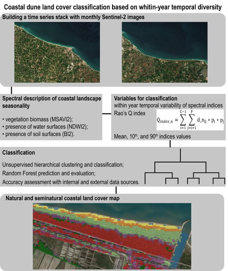
We followed an unsupervised approach and classified coastal dune natural and semi-natural land cover types through a hierarchical cluster analysis. The classes identified in the clustering phase were then used as the response variable in a Random Forest (RF) model (an accurate learning method for discriminating differences among classes [43,44]), in order to quantify their accuracy and to predict their occurrence in the study area. In particular, the procedure was organized in the following steps: (1) Sentinel-2 imagery selection; (2) spectral indices calculation and temporal variability computation; (3) variables selection and classification; (4) accuracy assessment (Figure 2).
2.2.1. Sentinel-2 Imagery Selection
We used Sentinel-2 mission images as a sound support for land monitoring [45], with good spatial (10, 20 or 60 m), temporal (revisit time of 2–3 days at mid-latitudes) and spectral (13 bands ranging from 400 nm to visible to 2400 nm) resolutions [25]. Multispectral images of Sentinel-2 satellites were downloaded from Copernicus Open Access Hub (https://scihub.copernicus.eu/) at the level of bottom of atmosphere (Level-2A), and used to build a monthly temporal dataset for the year 2019. As the study area falls in two tiles (T33TVG, T33TWG), we selected 24 images (12 for tile) of each month with low cloud coverage (<5%, Supplementary Material). All images were atmospherically corrected by ESA through the “sen2cor” processor algorithm (Figure 2, box 1) [46]. We specifically used Green band, with wavelength 560 ± 36 nm; Red band, with wavelength 665 ± 31 nm, and NIR band, with wavelength 833 ± 106 nm, with 10 m of resolution.
2.2.2. Spectral Indices Calculation and Temporal Variability Computation
For each image, we calculated three spectral indices: Modified Soil-Adjusted Vegetation Index 2 (MSAVI2), Normalized Difference Water Index 2 (NDWI2) and Brightness Index 2 (BI2), as they are good indicators of vegetation biomass, the presence of water surfaces, and bare surfaces, respectively (Figure 2 box 2 a, Table 1).
MSAVI2 is a vegetation index that quantifies the photosynthetic biomass based on Red and NIR bands (Table 1). MSAVI2 has been developed for mapping landscapes characterized by high percentages of bare surfaces [47,48] and its spatial behavior is a good support for land classification [49]. MSAVI2 ranges from −1 (absence of biomass vegetation) to 1 (maximum of biomass vegetation) with higher values indicating higher percentages of photosynthetic biomass [48].
NDWI2 is a water index that is useful to identify water surfaces, exploiting the Green and NIR bands (Table 1). NDWI2 is a remotely sensed index that is particularly efficient for identifying water surfaces and for mapping water-land transitions [50,51]. NIR band and Green band present opposite reflectance values behaviors and NDWI2 values range from −1 to 1, where values greater than 0 indicate water surfaces [52].
The BI2 index is sensitive to soil brightness, hence it quantifies the bare surfaces through the square root of brightness of each pixel (Table 1) [53]. BI2 accurately discriminates the bare surfaces from vegetation in heterogeneous environments [54,55]. The minimum value of BI2 is 0 and indicates the absence of bare surfaces, as growing positive values correspond to increasing percentages of bare surfaces.
We used ESA’s Sentinel-2 toolbox—ESA Sentinel Application Platform 7.0 (SNAP) for index calculation.
For each spectral index, we built an annual stack containing the 12 month values (i.e., MSAVI22019, NDWI22019, BI22019), standardized between 0 and 1 to make them comparable [56]. To summarize the within-year heterogeneity of ecological conditions (e.g., biomass, water surfaces and bare surfaces yearly variation), we calculated the temporal Rao’s Q index for each annual stack (Figure 2 box 2 b). The Rao’s Q index has recently been borrowed from functional ecology and successfully applied in remote sensing contexts as an innovative measure of spectral heterogeneity [36]. Such a proposed version of temporal Rao’s Q index accounts for both the relative abundances of the values assumed by a given pixel n throughout the temporal stack (e.g., 12 months), and the Euclidean distances among the pixel’s numerical values.
The Rao’s Q diversity index was applied on each annual stack (i.e., MSAVI22019, NDWI22019, and BI22019) according to the following formula (Equation (1)) [57,58]:
where:
Qindex_n = Rao’s Q quantifying the within-year variability of a spectral index (MSAVI22019, NDWI22019 or BI22019) for the pixel n
p = relative abundance of the index value assumed by the pixel n within a temporal stack
i = month i
j = month j
d_nij = distance between the month i-th and j-th index value of pixel n (dij = dji and dii = 0).
As similarly done in spectral diversity applications, Rao’s Q adapted to detect temporal diversity quantifies the expected dissimilarity between two combinations of pixel values randomly selected within a pixel temporal stack (Figure 3). Pixels representing highly seasonal cover types (e.g., deciduous or annual formations) are characterized by a pronounced within-year variability of biomass values and bare surfaces cover. Therefore, such pixels should assume high temporal Rao’s Q values. On the contrary, pixels representing temporally stable coastal areas (e.g., open sand, pine wood) portraying weak or absent seasonal variations, should score low Rao’s Q values. The temporal Rao’s Q for each spectral index (QMSAVI2, QNDWI2, QBI2) was computed through R package ‘spacetimerao’ 0.1 [59].
In order to summarize the range of annual variation for each index, we also calculated their mean values (MBI2, MMSAVI2, MNDWI2), along with their 10th and 90th percentiles (10thBI2, 10thMSAVI2, 10thNDWI2, 90thBI2, 90thMSAVI2, 90thNDWI2, Figure 2 box 2 c).
2.2.3. Variables Selection and Classification
The classification phase was implemented through consecutive cycles, each structured into three steps (Figure 2 box 3). Each step consists of a sequence of procedures: (a) variables selection, (b) pixel sampling and representativeness assessment, (c) clustering and classification. As covariates for classification, we used 12 variables, which describe the temporal heterogeneity (QMSAVI2, QNDWI2, QBI2), the central tendency (MMSAVI2, MNDWI2, MBI2), and the variation range (10thMSAVI2, 10thNDWI2, 10thBI2, 90thMSAVI2, 90thNDWI2, 90thBI2) of the three spectral indices (i.e., MSAVI2, NDWI2, BI2).
(a) Variables Selection
During each cycle, the 12 covariates were checked for their multicollinearity (Graham 2003) using the Variance Inflation Factor (VIF, Figure 2 box 3 a). VIF quantifies the multiple correlation of a variable with respect to all the other variables through linear regressions [60]. As VIF values greater than 5 indicate multicollinearity problems [61], we retained, for the analysis, the variables with VIF < 5 [62].
(b) Pixel Sampling and Representativeness Assessment
To reduce the computational costs, we ran the classification process on a subset of pixels randomly extracted from the study area. In particular, classification was carried out on a 20%-pixel sample and the results were extrapolated throughout the entire study area using an RF algorithm. The degree of extrapolation on values of covariates lying outside the RF calibration range was assessed through the Multivariate Environmental Similarity Surface, (MESS, Figure 2 box 3 b) [63]. MESS quantifies the similarity of all the pixels in the study area with respect to the covariates of the extracted 20% sample used for classification. Low MESS values indicate a high similarity between covariate values of calibration and prediction pixels, suggesting a high representativeness of the former. In each classification cycle, we indicated the percentage of highly dissimilar pixels (MESS value < 0).
(c) Clustering and Classification
The random sample of pixels was classified through a hierarchical cluster analysis using the Ward’s minimum variance method [64], which minimizes the cluster’s internal variability using the sum-of-squares [65,66]. We used as distance the Bray–Curtis dissimilarity metric [67,68] measured as follows (Equation (2))
where BCpq is the Bray–Curtis dissimilarity between pixels (p, q), xpi are the values of the n selected remotely sensed variables (e.g., QMSAVI2, MNDWI2, 90thBI2) on pixel p and xqi the variables value on pixel q. BCpq ranges from 0 when the pixels are identical, to 1 when the pixels are completely different [69].
On each cycle, we identified the optimal number of classes (form from 2 to 10 classes; Supplementary Material) by calculating three indices (Silhouette index [70]; Calinski–Harabasz index [71] and Davies–Bouldin index [72]) on the just built hierarchical cluster. The selected indices summarize two cluster characteristics: the compactness of classes (e.g., how closely pixels are grouped inside a class), and the separation between classes (e.g., how the classes are different from each other).
The classes identified in the clustering phase were used as response variables in a RF model (R package ‘caret’ 6.0-85; Supplementary Material) [73,74,75] in order to evaluate their accuracy, to extrapolate the classification throughout all the pixels of the study area, and to evaluate the variables’ contribution in defining such classes. To optimize RF parameters, we set a high number of uncorrelated decision trees (Ntree = 1000) [76,77,78], while testing different combinations of the number of variables randomly selected at each node (Mtry parameter) and split rules [79,80,81,82], then choosing the combination that yielded the highest Kappa statistic value. Specifically, we tested Mtry values ranging from 2 to the total number of variables in the cycle, and the Gini index and Extra-Trees algorithm as possible split rules (Supplementary Material).
Once the optimal RF model was identified, it was used to predict the membership of all the study area pixels to one of the classes identified in the clustering phase. Moreover, we estimated the relative variables’ importance (Supplementary Material) [83].
At the end of each cycle, we repeated the three steps (variables selection, pixel sampling and representativeness assessment, clustering and classification) inside the classified land cover classes.
The final classes predicted by the classification phase were then interpreted in terms of coastal cover types through an expert-based approach based on field detection and visual interpretation of high resolution aerial images (~1 m).
2.2.4. Accuracy Assessment
The RF predictive accuracy was assessed by an internal 10-fold cross validation and an independent validation based on 300 random checkpoints. We selected 300 points as to assure a minimum standard number of 20 control points for each land cover class [84]. In the independent accuracy assessment, we compared the assignment of the checkpoints according to the land cover classes obtained by satellite classification with their description obtained from field observations and the visual inspection of Google Earth images. Because of the differences in spatial resolution between Sentinel-2 (10 × 10 m) and Google Earth images (~1 m), we focused our visual inspection on circular buffer areas of 5-m radius (10 m’ diameter) around each check point [85,86,87,88]. In both accuracy assessments, we calculated the same performance metrics. We built a confusion matrix and calculated the percentages of overall accuracy, producer’s accuracy, user’s accuracy and Kappa statistic [84]. Moreover, we calculated the Matthews Correlation Coefficient, both overall and for each land cover class [89]. This coefficient is widely used to evaluate the accuracy of classifications [86,90], as it proved reliable to evaluate the accuracy of classification when the classes had different sizes; its range of −1 to 1 and values close to 1 represent a perfect accuracy [87,91].
3. Results
3.1. Unsupervised Classification
We obtained seven land cover classes after three classification cycles, which are organized in two hierarchical levels, with marked differences in temporal diversity values and in the range of the spectral indices (Figure 4 and Figure 5). During the first classification cycle, we identified the first hierarchical level including three classes (see Table 2, Figure S1): Water (W), Sand (S), and Vegetation (V, Figure 4, Table 2). The second and third classification cycles established the second hierarchical level in which sand and vegetation clusters were split into two and four classes, respectively (see Table 2). Particularly, the second RF cycle applied to Sand class (S) identified two categories (Table 2, Figure S2): Water Edge (WE) and Open Sand (OS; Figure 4 and Figure 5). The WE class represents the sea–land transition including the inter-tidal area, while OS includes dry sand dunes partially covered by sparse annual vegetation. In the third cycle, RF split the class Vegetation (V) into four categories (Table 2, Figure S3): Mobile Dune Herbaceous Vegetation (MDHV), Fixed Dune Herbaceous Vegetation with Sparse Shrub (FHVSS), Evergreen Woody Vegetation (EWV), and Deciduous and Humid Herbaceous Vegetation (DHHV, Figure 4 and Figure 5). Since we focused on terrestrial cover types, we did not explore the presence of sub-classes inside the Water class (Table 3). For each cycle, RF showed extremely low MESS values, suggesting no extrapolation effect on models’ predictions throughout the study area. These outcomes evidenced that the selected pixels for each classification cycle are representative of the study area.
3.2. Accuracy Assessment
In all the three cycles, the RF results achieved very high accuracy values according to both cross-validation and field assessments (Table 3).
For the first cycle, the overall accuracy, Kappa statistic and MCC indicate an almost perfect agreement under both assessments (Table 3). Similar results were also obtained by performance metrics by land cover classes. In the field accuracy assessment, both user’s and producer’s accuracy values in all classes are high, with the Sand class accuracy resulting lower than 90% (Table S3). The second classification cycle reported cross-validation performances of 99% for overall accuracies, 96% for Kappa statistic, and 0.98 for Matthews Correlation Coefficient, while the performance assessed through the field assessment is slightly lower (overall accuracy: 87%, Kappa statistic: 72%, Matthews Correlation Coefficient: 0.66, Table 3). All performance metrics by land cover classes calculated through cross-validation indicate an almost perfect agreement, whereas the comparison of the natural and semi-natural land cover map between the field and visual inspection shows a decrement of accuracy (Table S4). Indeed, the Water Edge class evidences an almost perfect agreement only for the Producer’s accuracy, while the agreement of User’s accuracy and Matthews Correlation Coefficient shows a substantial agreement (Producer’s accuracy: 96.67, User’s accuracy: 72.22, Matthews Correlation Coefficient: 0.66, Table S4). The Open Sand class displays a higher agreement than the previous class, and, only for the Matthews Correlation Coefficient, the agreement drops to under 0.70 (Table S4). Finally, the performance of the third classification cycle has very high results under cross-validation assessment, with all metrics above 95% (overall accuracy: 97%, Kappa statistic: 96%, Matthews Correlation Coefficient: 0.96), while in the field accuracy assessment, the overall metrics show a substantial agreement (Table 3). Similar to the previous cycles, all land cover classes were accurately predicted, as showed by cross-validation results (Table S5).
In the field accuracy assessment, the user’s accuracy of all classes shows substantially good performances, with the metrics values resulting higher than 75%, especially in the Mobile Dune Herbaceous Vegetation class (Table S5). Equally, in the producer’s accuracy, all classes show a substantial agreement, and the values are higher than 70%; indeed, the values range from the minimum of substantial agreement (73%) in Deciduous and Humid Herbaceous Vegetation to the maximum of almost perfect agreement (93%) in Fixed Dune Herbaceous Vegetation with Shrubs (Table S5).
3.3. Variables Importance
Among the most important variables in the first RF cycle, the 10th percentile of NDWI2 (10thNDWI2) showed a 63% importance, followed by the 10th percentile of BI2 (10thBI2) with 22%, the temporal Rao of NDWI2 (QNDWI2, 11%), and the temporal Rao of BI2 (QBI2,4%). Water class (W) is characterized by high values of 10thNDWI2 and QNDWI2 (Figure 4) and includes the sea, rivers, channels and wetland. In this class, the 10thBI2 shows overall low values and variability, while QBI2 and QMSAVI2 are close to zero. These features are also evident when inspecting the annual trend of each of the three spectral indices (MSAVI2, NDWI2 and BI2; Figure 4). For the Water class, NDWI2 values are above 0.5 in all months. The BI2 and the NDWI2 values are always lower than 0.25 and 0, respectively.
The most important variables in the second RF cycle are temporal Rao of MSAVI2 (63%, QMSAVI2) followed by temporal Rao of BI2 (26%, QBI2) and the 90th percentile of BI2 (11%, 90thBI2, Table 2). Water Edge and Open Sand showed similar trends in annual spectral indices (Figure 4 and Figure 5), only differing in the upper values of brightness (90thBI2), which is higher in Open Sand. Open Sand shows higher BI2 values in summer (Figure 4), and lower variability in the upper values of biomass (90thMSAVI2, Figure 4).
The most important variables in the third RF cycle are the lower values of bare surfaces (10thBI2, 33%) and the temporal variability of biomass (QMSAVI2, 32%) and of bare surfaces (QBI2, 26%, Table 2). Mobile Dune Herbaceous Vegetation (MDHV, Figure 4 and Figure 5) is characterized by high values of bare surfaces (high 10thBI2 and low Q BI2) and moderate values of biomass (low MMSAVI2 and low QMSAVI2). The MSAVI2 index profile depicts a mosaic of bare sand with sparse open perennial and annual vegetation that corresponds to coastal herbaceous vegetation referable to mobile dunes (Figure 5). Fixed Dune Herbaceous Vegetation with Shrubs (FDHVS, Figure 4 and Figure 5) is characterized by a strong seasonality (intermediate MMSAVI2 and very high QMSAVI2), intermediate biomass values and moderate presence of bare surfaces (moderate 10thBI2 and QBI2) and water (moderate QNDWI2). The FDHVS corresponds to herbaceous vegetation with shrubs growing on fixed dunes and dune slacks, more inland with respect to the previous class of ruderal vegetation. Evergreen Woody Vegetation (EWV, Figure 4 and Figure 5) is characterized by high biomass values, a low seasonality (intermediate MMSAVI2 and very low QMSAVI2) and almost no bare surfaces (very low 10thBI2 and QBI2). EWV includes the Mediterranean maquis, pine woods and shrubs and woody evergreen formations. The Deciduous and Humid Herbaceous Vegetation class (DHHV, Figure 4 and Figure 5) is characterized by high biomass values and pronounced phenology (very high MMSAVI2 and very high QMSAVI2), as well as moderate bare surfaces occurrence (moderate 10thBI2 and QBI2). The DHHV includes herbaceous and woody vegetation of humid areas close to river mouths, riparian vegetation and residual patches of lowland woods.
4. Discussion
In this study, we used information from annual fluctuations of vegetation biomass, water surface, and bare soil combined into the temporal Rao’s Q index, in an effort to identify and map seven land cover classes that clearly depicted the sequence of coastal dune natural and semi-natural ecosystems occurring along the sea–inland gradient.
Our modelling approach showed high levels of classification accuracy, substantially confirming the usefulness of time-series analysis for semi-natural and natural land cover mapping [16,92,93]. Moreover, we pointed out the high potential of integrating such spectral indices as MSAVI2, NDWI2 and BI2 to describe land cover seasonality in such heterogeneous environments as those of coastal dunes.
The classification framework that made it possible to identify and map seven coastal semi-natural cover types was organized in two hierarchical levels. For each set of cover types, different variables emerged as the most important for classification. In the first RF cycle implemented on the overall coastal landscape, water surface was split from the other cover classes because of the typical behavior of water-related spectral indices. Specifically, the minimum of NDWI2 (10thNDWI2) and its temporal diversity (QNDWI2) assumed particularly high values and emerged as the most important variables in the first RF cycle. As previously observed, the spectral responses of water and dryland are very different [94,95]. Such differences clearly emerged at coarser classification levels on the transition area we analyzed here. However, the percentage of bare surfaces also appeared as an important variable in the first cycle, revealing the presence of open sand and sparse vegetation in the coastal dune mosaic. In the second and third cycles performed on non-water areas, the temporal diversity of biomass (QMSAVI2) showed an important role in land cover classification, confirming the importance of phenology in coastal landscape mapping [16]. In particular, the second cycle, which focused on open sand and sparse vegetation areas, reported the phenology (QMSAVI2) along with the annual fluctuations on bare soil (QBI2) as important variables discriminating bare areas from complex mosaics of pioneer vegetation and sand [96,97]. The third RF cycle focused mainly on vegetated areas hosting herbaceous and woody land cover classes, reporting the temporal variability of vegetation biomass (QMSAVI2) and the low percentages of bare soil (10thBI2) as the most important predictors for classification. In addition, low temporal variation on bare soil cover (low QBI2) helped to discriminate seasonal deciduous formations from the contiguous evergreen vegetation [38,96].
The classification of Rao’s Q temporal diversity measured on spectral indices made it possible to identify and map the mosaic characterizing the different sectors of coastal dune zonation with high accuracy levels. However, such transition classes as Water Edge and Fixed Dune Herbaceous Vegetation with Shrubs evidenced the lowest values, perhaps due to the spatial dimension of Sentinel-2 images (10 m), which is too coarse to describe this intricate transition mosaic.
The seven identified classes clearly depicted the sequence of coastal dune natural and semi natural cover classes occurring from the sea to the inland, each characterized by a specific seasonal pattern. Indeed, classes ranged from the Water class including the sea close to the seashore, to Deciduous formations and Humid Herbaceous Vegetation growing in the inner dune slacks [16,41,92]. As for the Water Edge class, it represented the inter-tidal area, with higher presence of water during the winter months possibly caused by storms. The Open Sand class included the dry sand beach with the sparse annual vegetation on the drift line, while the embryonic shifting dune formations, such as the Dense Herbaceous Vegetation type, represented the mobile dunes with Ammophila arenaria (see also [16]). The Fixed Dune Herbaceous Vegetation with Shrubs class included a fine mosaic of herbaceous and shrub vegetation occurring on transition areas, as well as fuzzy edges between herbaceous and woody vegetation on dune sectors towards the sea and shrubs, and ruderal formations on inland disturbed areas [16,96]. As for the Evergreen Woody Vegetation class, we reported low temporal diversity values, both in vegetation biomass (QMSAVI2) and bare surfaces (QBI2), confirming the already known absence of seasonality of this cover class [16,98]. The Deciduous and Humid Herbaceous Vegetation class enclosed riparian deciduous woody vegetation and vegetation of humid environments. This class was characterized by a similar seasonality of vegetation biomass and presented two peaks in spring and summer that alternate with lower values in autumn and winter [99,100].
The results we obtained in this study clearly identified remotely sensed seasonality and Rao’s Q temporal diversity as an effective source of information for landscape mapping in coastal areas. Using Sentinel-2 images with accurate spatial, temporal and spectral resolutions [25], we derived sound temporal heterogeneity variables for land cover mapping summarizing spectral indices previously implemented separately (e.g., using MSAVI2 [48], or NDWI2 [52], or BI2 [53]).
Land cover classification based on multi-temporal remotely sensed data analysis has improved here for landscape mapping on Mediterranean coasts by relying on a set spectral indices rarely analyzed together, as well as by the introduction of Rao’s Q for summarizing their temporal variability. Furthermore, the implemented RF classification organized in sequential cycles ensured accurate and ecologically coherent results. For instance, water presence and seasonality evidenced by the yearly behavior of NDWI2 were important variables in the first cycle of classification implemented on overall coastal area extent, which confirmed its potential for discriminating water from emerged areas [94,95] and suggested its role when mapping transition systems between terrestrial and marine realms. Similarly, our results confirmed that biomass and bare soil indexes and their temporal variability are important variables for mapping terrestrial cover classes [16,28,92,101]. Based on our results, it possible to affirm that for remotely sensed monitoring and mapping, the inclusion of variables depicting bare soil, water and biomass seasonality are highly advisable.
5. Conclusions
The proposed procedure for classifying and mapping natural and semi-natural land cover effectively summarized the dynamic nature of coastal systems, capturing all of the main components of coastal dune mosaics together with their seasonal variation (i.e., vegetation, bare surfaces and water surfaces) by combining spectral indices that are rarely used together (MSAVI2, NDWI2, or BI2).
The information provided by Rao’s Q offered a sound base for natural and semi-natural land cover monitoring and mapping. In particular, the here proposed implementation of Rao’s Q temporal heterogeneity allowed the accurate depiction of the seasonality of the different cover types conforming the coastal dune mosaic along the sea–inland gradient (e.g., biomass phenology, water seasonality, yearly variation on bare surfaces). Furthermore, the applicability of the proposed framework on the available updated sentinel images emphasized the procedure as a promising tool for cover monitoring and reporting. Even more interestingly, the integration of other remotely sensed data with higher spatial resolutions derived by satellite, such as Planet images, UAV, or LiDAR data, may further improve the classification of coastal zonation.
From an applied perspective, the natural and semi-natural land cover map provided in this study yields relevant knowledge for coastal monitoring and management; therefore, we hope new studies exploring increasingly larger areas will be analyzed to further test the proposed classification and, at the same time, to provide homogeneous information for coasts in the Mediterranean.
Supplementary Materials
The following are available online at https://www.mdpi.com/2072-4292/12/14/2315/s1, Table S1: Sentinel-2 dataset indicating for each image the month, day, platform (Sentinel-2A or Sentinel-2B) and the hour of acquisition, the cloud percentage, and the relative tile (T33TVG for Molise north, T33TWF for Molise south). Table S2: The optimal number of classes for each cycle was identified by Silhouette, Calinski–Harabasz, and Davies–Bouldin indices calculated on a specific hierarchical cluster produced through Ward’s minimum variance. These three indices identify the optimal number of classes by comparing the intra-class compactness (degree of aggregation between pixels inside each class) and the separation between classes (degree of differences between classes). We fixed as the optimal number of classes, the most frequent output produced by the three indexes. Figure S1: Graphical representation of the Silhouette, Calinski–Harabasz, and Davies–Bouldin indices used for identifying the optimal number of classes in the 1° cycle of Random Forest. All three of the indices identified three as the optimal number of classes. Figure S2: Graphical representation of Silhouette, Calinski–Harabasz, and Davies–Bouldin indices used for identifying the optimal number of classes in the 2° cycle of Random Forest. Two (Silhouette and Calinski–Harabasz) of the three indices have established two as the optimal number of classes. Figure S3: Graphical representation of Silhouette, Calinski–Harabasz, and Davies–Bouldin indices used for identifying the optimal number of classes in the 3° cycle of Random Forest. Two (Silhouette and Calinski–Harabasz) of the three indices suggested four as the optimal number of classes. Table S3: The percentages of accuracy assessment values by land cover classes for first classification cycle: Water (W), Sand (S), Vegetation (V). In particular, User’s accuracy (U ACC), Producer’s accuracy (P ACC), and Matthews Correlation Coefficient (MCC). In the Random Forest accuracy assessment are indicated the mean values and standard deviation for the performance metrics. Table S4: The percentages of accuracy assessment values by land cover classes for second classification cycle: Water Edge (WE), Open Sand (OS). In particular, User’s accuracy (U ACC), Producer’s accuracy (P ACC), and Matthews Correlation Coefficient (MCC). In the Random Forest accuracy assessment are indicated the mean values and standard deviation for the performance metrics. Table S5: The percentages of accuracy assessment values by land cover classes for the third classification cycle: Dense Herbaceous Vegetation (DHV), Evergreen Woody Vegetation (EWV), Fixed Dune Herbaceous Vegetation with Shrubs (FDHVS), Deciduous and Humid Herbaceous Vegetation (DHHV). In particular, User’s accuracy (U ACC), Producer’s accuracy (P ACC), and Matthews Correlation Coefficient (MCC). In the Random Forest accuracy assessment are indicated the mean values and standard deviation for the performance metrics.
Author Contributions
All authors contributed substantially to the work: F.M., M.M. and M.L.C. conceived and designed the study; F.M. collected the data; F.M., M.D.F., M.L.C. analyzed the data; F.M., M.M., S.G., M.L.C. led the writing of the manuscript; A.T.R.A. and M.L.C. supervised the research. All authors contributed critically to the drafts and gave final approval for publication. All authors have read and agreed to the published version of the manuscript.
Funding
This research received no external funding.
Acknowledgments
This study was carried out with the partial support of PON-AIM (Italian program for research and innovation 2014-2020—AIM1897595-2) in collaboration with the bilateral program Italy–Israel DERESEMII (Developing state-of-the-art remote sensing tools for monitoring the impact of invasive plant species in coastal ecosystems in Israel and Italy) and INTERREG Italy-Croazia CASCADE (CoAStal and marine waters integrated monitoring systems for ecosystems proteCtion AnD management - Project ID 10255941). The authors acknowledge the Principal Investigator(s) of the Sentinel-2 mission for providing datasets in the archive and the developers of SNAP software used for data analysis. Sentinel-2 images are freely downloadable from the Copernicus Open Access Hub https://scihub.copernicus.eu/). Furthermore, the authors acknowledge the entire team of EnvixLab, in particular Ludovico Frate, Gabriella Sferra, Marco Varricchione, Luca Francesco Russo, for the help given. The authors also thank the editor and the anonymous reviewers for their comments that helped us to improve the manuscript.
Conflicts of Interest
The authors declare no conflict of interest.
References
- Allan, E.; Manning, P.; Alt, F.; Binkenstein, J.; Blaser, S.; Blüthgen, N.; Böhm, S.; Grassein, F.; Hölzel, N.; Klaus, V.H.; et al. Land use intensification alters ecosystem multifunctionality via loss of biodiversity and changes to functional composition. Ecol. Lett. 2015, 18, 834–843. [Google Scholar] [CrossRef] [PubMed]
- Mantyka-Pringle, C.S.; Visconti, P.; Di Marco, M.; Martin, T.G.; Rondinini, C.; Rhodes, J.R. Climate change modifies risk of global biodiversity loss due to land-cover change. Biol. Conserv. 2015, 187, 103–111. [Google Scholar] [CrossRef] [Green Version]
- Oliver, T.H.; Heard, M.S.; Isaac, N.J.B.; Roy, D.B.; Procter, D.; Eigenbrod, F.; Freckleton, R.; Hector, A.; Orme, C.D.L.; Petchey, O.L.; et al. Biodiversity and resilience of ecosystem functions. Trends Ecol. Evol. 2015, 30, 673–684. [Google Scholar] [CrossRef] [PubMed] [Green Version]
- Brown, A.C.; McLachlan, A. Sandy shore ecosystems and threats facing them: Some predictions for the year 2025. Environ. Conserv. 2002, 29, 62–77. [Google Scholar] [CrossRef] [Green Version]
- Defeo, O.; McLachlan, A.; Schoeman, D.S.; Schlacher, T.A.; Dugan, J.; Jones, A.; Lastra, M.; Scapini, F. Threats to sandy beach ecosystems: A review. Estuar. Coast. Shelf Sci. 2009, 81, 1–12. [Google Scholar] [CrossRef]
- Martínez, M.L.; Psuty, N.P. Coastal Dunes. Ecology and Conservation, 2nd ed.; Springer: Berlin/Heidelberg, Germany, 2008; pp. 1–387. [Google Scholar]
- Martínez, M.L.; Intralawan, A.; Vázquez, G.; Pérez-Maqueo, O.; Sutton, P.; Landgrave, R. The coasts of our world: Ecological, economic and social importance. Ecol. Econ. 2007, 63, 254–272. [Google Scholar] [CrossRef]
- Drius, M.; Jones, L.; Marzialetti, F.; de Francesco, M.C.; Stanisci, A.; Carranza, M.L. Not just a sandy beach. The multi-service value of Mediterranean coastal dunes. Sci. Total Environ. 2019, 668, 1139–1155. [Google Scholar] [CrossRef] [Green Version]
- Hesp, P.A. Ecological processes and plant adaptations on coastal dunes. J. Arid Environ. 1991, 21, 165–191. [Google Scholar] [CrossRef]
- Acosta, A.T.R.; Blasi, C.; Carranza, M.L.; Ricotta, C.; Stanisci, A. Quantifying ecological mosaic connectivity and hemeroby with a new topoecological index. Phytocoenologia 2003, 33, 623–631. [Google Scholar] [CrossRef]
- Henle, K.; Bauch, B.; Auliya, M.; Külvik, M.; Pe‘er, G.; Schmeller, D.S.; Framstad, E. Priorities for biodiversity monitoring in Europe: A review of supranational policies and a novel scheme for integrative prioritization. Ecol. Indic. 2013, 33, 5–18. [Google Scholar] [CrossRef]
- Janssen, J.A.M.; Rodwell, J.S.; García Criado, M.; Gubbay, S.; Haynes, T.; Nieto, A.; Sanders, N.; Landucci, F.; Loidi, J.; Ssymank, A.; et al. European Red List of Habitats. Part 2. Terrestrial and Freshwaters Habitats; European Union: Luxemburg, 2016; pp. 1–38. [Google Scholar]
- Acosta, A.T.R.; Carranza, M.L.; Izzi, C.F. Combining land cover mapping of coastal dunes with vegetation analysis. Appl. Veg. Sci. 2005, 8, 133–138. [Google Scholar] [CrossRef]
- Malavasi, M.; Santoro, R.; Cutini, M.; Acosta, A.T.R.; Carranza, M.L. What has happened to coastal dunes in the last half century? A multitemporal coastal landscape analysis in Central Italy. Landsc. Urban Plan. 2013, 119, 54–63. [Google Scholar] [CrossRef]
- Brownett, J.M.; Mills, R.S. The development and application of remote sensing to monitor sand dune habitats. J. Coast. Conserv. 2017, 21, 643–655. [Google Scholar] [CrossRef] [Green Version]
- Marzialetti, F.; Giulio, S.; Malavasi, M.; Sperandii, M.G.; Acosta, A.T.R.; Carranza, M.L. Capturing coastal dune natural vegetation types using a phenology-based mapping approach: The potential of Sentinel-2. Remote Sens. 2019, 11, 1506. [Google Scholar] [CrossRef] [Green Version]
- Doody, J.P. Sand Dune Conservation Management and Restoration, 1st ed.; Springer: Dordrecht, The Netherlands, 2013; pp. 9–20. [Google Scholar]
- Williams, C.M.; Ragland, G.J.; Betini, G.; Buckley, L.B.; Cheviron, Z.A.; Donohue, K.; Hereford, J.; Humphries, M.M.; Lisovski, S.; Marshall, K.E.; et al. Understanding evolutionary impacts of seasonality: An introduction to the symposium. Integr. Comp. Biol. 2017, 57, 921–933. [Google Scholar] [CrossRef] [PubMed]
- Tonkin, J.D.; Bogan, M.T.; Bonada, N.; Rios-Touma, B.; Lytle, D.A. Seasonality and predictability shape temporal species diversity. Ecology 2017, 98, 1201–1216. [Google Scholar] [CrossRef] [Green Version]
- Gómez, C.; White, J.C.; Wulder, M.A. Optical remotely sensed time series data for land cover classification: A review. ISPRS J. Photogramm. Remote Sens. 2016, 116, 55–72. [Google Scholar] [CrossRef] [Green Version]
- Senf, C.; Leitão, P.J.; Pflugmacher, D.; van der Linden, S.; Hostert, P. Mapping land cover in comlex Mediterranean landscapes using Landsat: Improved classification accuracies from integrating multi-seasonal and synthetic imagery. Remote Sens. Environ. 2015, 156, 527–536. [Google Scholar] [CrossRef]
- Luo, J.; Li, X.; Ma, R.; Li, F.; Duan, H.; Hu, W.; Qin, B.; Huang, W. Applying remote sensing techniques to monitoring seasonal and interannual changes of acquatic vegetation in Taihu Lake, China. Ecol. Indic. 2016, 60, 503–513. [Google Scholar] [CrossRef]
- Mannel, S.; Price, M. Comparing classification results of multi-seasonal TM against AVIRIS imagery-seasonality more important then number of bands. Photogramm. Fernerkund. Geoinf. 2012, 5, 603–612. [Google Scholar] [CrossRef]
- Knight, J.F.; Luneta, R.S.; Ediriwickrema, J.; Khorran, S. Regional scale land cover characterization using MODIS-NDVI 250 m multi-temporal imagery: A phenology-based approach. GIScience Remote Sens. 2006, 43, 1–23. [Google Scholar] [CrossRef]
- Drusch, M.; Del Bello, U.; Carlier, S.; Colin, O.; Fernandez, V.; Gascon, F.; Hoersch, B.; Isola, C.; Labertini, P.; Martimort, P.; et al. Sentinel-2: ESA’s optical high-resolution mission for GMES operational services. Remote Sens. Environ. 2012, 120, 25–36. [Google Scholar] [CrossRef]
- Wulder, M.A.; Hilker, T.; White, J.C.; Coops, N.C.; Masek, J.G.; Pflugmacher, D.; Crevier, Y. Virtual constellations for global terrestrial monitoring. Remote Sens. Environ. 2015, 170, 65–76. [Google Scholar] [CrossRef] [Green Version]
- Hill, R.A.; Wilson, A.K.; George, M.; Hinsley, S.A. Mapping tree species in temperate deciduous woodland using time-series multi-spectral data. Appl. Veg. Sci. 2010, 13, 86–99. [Google Scholar] [CrossRef]
- Rapinel, S.; Mony, C.; Lecoq, L.; Clénìment, B.; Thomas, A.; Hubert-Moy, L. Evaluation of Sentinel-2 time-series for mapping floodplain grassland plant communities. Remote Sens. Environ. 2019, 223, 115–129. [Google Scholar] [CrossRef]
- Noormets, A. Phenology of Ecosystem Processes. Applications in Global Change Research, 1st ed.; Springer: New York, NY, USA, 2009; pp. 1–275. [Google Scholar]
- Donohue, R.J.; McVicar, T.R.; Roderick, M.L. Climate-related trends in Australian vegetation cover as inferred from satellite observations, 1981–2006. Glob. Chang. Biol. 2009, 15, 1025–1039. [Google Scholar] [CrossRef]
- Rocchini, D.; Marcantonio, M.; Da Re, D.; Chirici, G.; Galluzzi, M.; Lenoir, J.; Ricotta, C.; Torresani, M.; Ziv, G. Time-lapsing biodiversity: And open source method for measuring diversity changes by remote sensing. Remote Sens. Environ. 2019, 231, 111192. [Google Scholar] [CrossRef] [Green Version]
- Torresani, M.; Rocchini, D.; Sonnenschein, R.; Zebisch, M.; Marcantonio, M.; Ricotta, C.; Tonon, G. Estimating tree species diversity from space in an alpine conifer forest: The Rao’s Q diversity index meets the spectral variation hypothesis. Ecol. Inform. 2019, 52, 26–34. [Google Scholar] [CrossRef] [Green Version]
- Ricotta, C.; Carranza, M.L.; Avena, G.; Blasi, C. Quantitative comparison of the diversity of landscapes with actual vs. potential natural vegetation. Appl. Veg. Sci. 2000, 3, 157–162. [Google Scholar] [CrossRef]
- Ricotta, C.; Moretti, M. CWM and Rao’s quadratic diversity: A unified framework for functional ecology. Oecologia 2011, 167, 181–188. [Google Scholar] [CrossRef]
- Ricotta, C.; Carranza, M.L. Measuring scale-dependent landscape structure with Rao’s quadratic diversity. ISPRS Int. J. Geo-Inf. 2013, 2, 405–412. [Google Scholar] [CrossRef] [Green Version]
- Rocchini, D.; Marcantonio, M.; Ricotta, C. Measuring Rao’s Q diversity index from remote sensing: An open source solution. Ecol. Indic. 2017, 72, 234–238. [Google Scholar] [CrossRef]
- Acosta, A.T.R.; Carranza, M.L.; Izzi, C.F. Are there habitats that contribute best to plant species diversity in coastal dunes? Biodivers. Conserv. 2009, 18, 1087–1098. [Google Scholar] [CrossRef]
- Carranza, M.L.; Acosta, A.T.R.; Stanisci, A.; Pirone, G.; Ciaschetti, G. Ecosystem classification for EU habitat distribution assessment in sandy coastal environments: An application in central Italy. Environ. Monit. Assess. 2008, 140, 99–107. [Google Scholar] [CrossRef]
- Stanisci, A.; Acosta, A.T.R.; Carranza, M.L.; Feola, S.; Giuliano, M. Gli habitat di interesse comunitario sul litorale molisano e il loro valore naturalistico su base floristica. Fitosociologia 2007, 44, 171–175. [Google Scholar]
- Drius, M.; Malavasi, M.; Acosta, A.T.R.; Ricotta, C.; Carranza, M.L. Boundary-based analysis for the assessment of coastal dune landscape integrity over time. Appl. Geogr. 2013, 45, 41–48. [Google Scholar] [CrossRef]
- Stanisci, A.; Acosta, A.T.R.; Carranza, M.L.; de Chiro, M.; Del Vecchio, S.; Di Martino, L.; Frattaroli, A.R.; Fusco, S.; Izzi, C.F.; Pirone, G.; et al. EU habitats monitoring along the coastal dunes of the LTER sites of Abruzzo and Molise (Italy). Plant Sociol. 2014, 51, 51–56. [Google Scholar] [CrossRef]
- Prisco, I.; Stanisci, A.; Acosta, A.T.R. Mediterranean dunes on the go: Evidence from a short term study on coastal herbaceous vegetation. Estuar. Coast. Shelf Sci. 2016, 182, 40–46. [Google Scholar] [CrossRef]
- Gislason, P.O.; Benediktsson, J.A.; Sveinsson, J.R. Random forests for land cover classification. Pattern Recognit. Lett. 2006, 27, 294–300. [Google Scholar] [CrossRef]
- Pal, M. Random forest classifier for remote sensing classification. Int. J. Remote Sens. 2005, 26, 217–222. [Google Scholar] [CrossRef]
- Berger, M.; Moreno, J.; Johannessen, J.A.; Levelt, P.F.; Hanssen, R.F. ESA’s sentinel missions in support of Earth system science. Remote Sens. Environ. 2012, 120, 84–90. [Google Scholar] [CrossRef]
- Main-Knorn, M.; Pflug, B.; Louis, J.; Debaecker, V.; Müller-Wilm, U.; Gascon, F. Sen2Cor for Sentinel-2. In Image and Signal Processing for Remote Sensing XXIII, Proceedings of Spie Remote Sensing, Warsaw, Poland, 21–24 September; Bruzzone, L., Bovolo, F., Eds.; SPIE: Bellingham, WA, USA, 2017. [Google Scholar]
- Rondeaux, G.; Steven, M.; Baret, F. Optimization of soil-adjusted vegetation indices. Remote Sens. Environ. 1996, 55, 95–107. [Google Scholar] [CrossRef]
- Qi, J.; Chehbouni, A.; Huete, A.R.; Kerr, Y.H.; Sorooshian, S. A modified soil adjusted vegetation index. Remote Sens. Environ. 1994, 48, 118–126. [Google Scholar] [CrossRef]
- Wu, Z.; Velasco, M.; McVay, J.; Middleton, B.; Vogel, J.; Dye, D. MODIS derived vegetation index for drought detection on the San Carlos Apache reservation. Int. J. Adv. Remote Sens. GIS 2016, 5, 1524–1538. [Google Scholar] [CrossRef] [Green Version]
- Adam, E.; Mutanga, O.; Rugege, D. Multispectral and hyperspectral remote sensing for identification and mapping of wetland vegetation: A review. Wetl. Ecol. Manag. 2010, 18, 281–296. [Google Scholar] [CrossRef]
- Maglione, P.; Parente, C.; Vallario, A. Coastline extraction using high resolution WorldView-2 satellite imagery. Eur. J. Remote Sens. 2014, 47, 685–699. [Google Scholar] [CrossRef]
- McFeeters, S.K. The use of the Normalized Difference Water Index (NDWI) in the delineation of open water features. Int. J. Remote Sens. 1996, 17, 1425–1432. [Google Scholar] [CrossRef]
- Escadafal, R. Remote sensing of soil color: Principles and applications. Remote Sens. Rev. 1989, 7, 261–279. [Google Scholar] [CrossRef]
- Todd, S.W.; Hoffer, R.M.; Milchunas, D.G. Biomass estimation on grazed and ungrazed rangelands using spectral indices. Int. J. Remote Sens. 1998, 19, 427–438. [Google Scholar] [CrossRef]
- Timm, B.C.; McGarigal, K. Fine-scale remotely-sensed cover mapping of coastal dune and salt marsh ecosystems at Cape Cod National Seashore using Random Forests. Remote Sens. Environ. 2012, 127, 106–117. [Google Scholar] [CrossRef]
- Milligan, G.W.; Cooper, M.C. A study of standardization of variables in cluster analysis. J. Classif. 1988, 5, 181–204. [Google Scholar] [CrossRef]
- Rocchini, D.; Balkenhol, N.; Carter, G.M.; Foody, G.M.; Gillespie, T.W.; He, K.S.; Kark, S.; Levin, N.; Lucas, K.; Luoto, M.; et al. Remotely sensed spectral heterogeneity as a proxy of species diversity: Recent advances and open challenges. Ecol. Inform. 2010, 5, 318–319. [Google Scholar] [CrossRef]
- Rao, C.R. Diversity and dissimilarity coefficients: A unified approach. Theor. Popul. Biol. 1982, 21, 24–43. [Google Scholar] [CrossRef]
- Bascietto, M. Compute Rao’s Diversity Index on Numeric Vectors and Matrices, R Package Version 0.1.0. 2018. Available online: https://github.com/mbask/spacetimerao/ (accessed on 28 September 2019).
- Zuur, A.F.; Ieno, E.N.; Elphick, C.S. A protocol for data exploration to avoid common statistical problems. Methods Ecol. Evol. 2010, 1, 3–14. [Google Scholar] [CrossRef]
- Chatterjee, S.; Hadi, A.S. Regression Analysis by Example, 5th ed.; John Wiley & Sons, Inc.: Hoboken, NJ, USA, 2012; pp. 248–251. [Google Scholar]
- Montgomery, D.C.; Peck, E.A.; Vining, G. Introduction to Linear Regression Analysis, 5th ed.; John Wiley & Sons Inc.: Hoboken, NJ, USA, 2012; pp. 1–645. [Google Scholar]
- Elith, J.; Kearney, M.; Philips, S. The art of modelling range-shifting species. Methods Ecol. Evol. 2010, 1, 330–342. [Google Scholar] [CrossRef]
- Ward, J.H. Hierarchical grouping to optimize and objective function. J. Am. Stat. Assoc. 1963, 58, 236–244. [Google Scholar] [CrossRef]
- Legendre, P.; Legendre, L. Numerical Ecology, 3rd ed.; Elsevier: Oxford, UK, 2012; pp. 360–367. [Google Scholar]
- Murtagh, F.; Legendre, P. Ward’s hierarchical agglomerative clustering method: Which algorithms implement ward’s criterion? J. Classif. 2014, 31, 274–295. [Google Scholar] [CrossRef] [Green Version]
- Bray, J.R.; Curtis, J.T. An ordination of the upland forest communities of Southern Wisconsin. Ecol. Monogr. 1957, 27, 325–349. [Google Scholar] [CrossRef]
- Goslee, S.C. Correlation analysis of dissimilarity matrices. Plant Ecol. 2010, 206, 279–286. [Google Scholar] [CrossRef]
- Ricotta, C.; Podani, J. On some properties of the Bray-Curtis dissimilarity and their ecological meaning. Ecol. Complex. 2017, 31, 201–205. [Google Scholar] [CrossRef]
- Kaufman, L.; Rousseeuw, P.J. Finding Groups in Data, 10th ed.; John Wiley & Sons: New York, NY, USA, 2005; pp. 1–342. [Google Scholar]
- Calinski, T.; Harabasz, J. A dendrite method for cluster analysis. Commun. Stat. Theory Methods 1974, 3, 1–27. [Google Scholar] [CrossRef]
- Davies, D.; Bouldin, D. A cluster separation measure. IEEE Trans. Pattern Anal. Mach. Intell. 1979, 1, 224–227. [Google Scholar] [CrossRef]
- Breiman, L. Random Forest. Mach. Learn. 2001, 45, 5–32. [Google Scholar] [CrossRef] [Green Version]
- Breiman, L.; Friedman, J.H.; Olshen, R.A.; Stone, C.J. Classification and Regression Trees, 3rd ed.; Chapman & Hall: Boca Ration, FL, USA, 1984; pp. 1–358. [Google Scholar]
- Kuhn, M.; Wing, J.; Weston, S.; Williams, A.; Keefer, C.; Engelhardt, A.; Cooper, T.; Mayer, Z.; Kenkel, B.; Benesty, M. Classification and Regression Training, R Package Version 6.0-85. 2020. Available online: https://github.com/topepo/caret/ (accessed on 28 September 2019).
- Kattenborn, T.; Lopatin, J.; Förster, M.; Braun, A.C.; Fassnacht, F.E. UAV data as alternative to field sampling to map woody invasive species based on combined Sentinel-1 and Sentinel-2 data. Remote Sens. Environ. 2019, 227, 61–73. [Google Scholar] [CrossRef]
- Colditz, R.R. An evaluation of different training sample allocation schemes for discrete and continuous land cover classification using decision tree-based algorithms. Remote Sens. 2015, 7, 9655–9681. [Google Scholar] [CrossRef] [Green Version]
- Lawrence, R.L.; Wood, S.D.; Sheley, R.L. Mapping invasive plans using hyperspectral imagery and Breiman Cutler classifications (RandomForest). Remote Sens. Environ. 2006, 100, 356–362. [Google Scholar] [CrossRef]
- Noi, P.T.; Kappas, M. Comparison of Random Forest, k-Nearest Neighbor and Support Vector Machine classifiers for land cover classification using Sentinel-2 imagery. Sensors 2018, 18, 18. [Google Scholar] [CrossRef] [Green Version]
- Belgiu, M.; Drăgut, L. Random forest in remote sensing: A review of applications and future directions. ISPRS J. Photogramm. Remote Sens. 2016, 114, 24–31. [Google Scholar] [CrossRef]
- Gastwirth, J.L. The estimation of the Lorenz curve and Gini index. Rev. Econ. Stat. 1972, 54, 306–316. [Google Scholar] [CrossRef]
- Geurts, P.; Ernest, D.; Wehenkel, L. Extremely randomized trees. Mach. Learn. 2006, 63, 3–42. [Google Scholar] [CrossRef] [Green Version]
- Cutler, D.R.; Edwards, T.C.; Beard, K.H.; Cutler, A.; Hess, K.T.; Gibson, J.; Lawler, J.J. Random forests for classification in ecology. Ecology 2007, 88, 2783–2792. [Google Scholar] [CrossRef] [PubMed]
- Congalton, R.G.; Green, K. Assessing the Accuracy of Remotely Sensed Data. Principles and Practices, 2nd ed.; CRC Press and Taylor & Francis Group: Boca Raton, FL, USA, 2009; pp. 1–183. [Google Scholar]
- Dorais, A.; Cardille, J. Strategies for incorporating high-resolution Google Earth databases to guide and validate classifications: Understanding deforestation in Borneo. Remote Sens. 2011, 3, 1157–1176. [Google Scholar] [CrossRef] [Green Version]
- Mohammed, N.Z.; Landry, R., Jr. Assessing horizontal positional accuracy of Google Earth imagery in the city of Montreal, Canada. Geod. Cartogr. 2016, 43, 55–65. [Google Scholar] [CrossRef] [Green Version]
- Tilahun, A.; Teferie, B. Accuracy assessment of land use land cover classification using Google Earth. Am. J. Environ. Prot. 2015, 4, 193–198. [Google Scholar] [CrossRef]
- Rwanga, S.S.; Ndambuki, J.M. Accuracy assessement of land use/land cover classification using remote sensing and GIS. Int. J. Geosci. 2017, 8, 611–622. [Google Scholar] [CrossRef] [Green Version]
- Matthews, B.W. Comparison of the predicted and observed secondary structure of T4 phage lysozyme. Biochim. Biophys. Acta (BBA) Protein Struct. 1975, 405, 442–451. [Google Scholar] [CrossRef]
- Boughorbel, S.; Jarray, F.; El-Anbari, M. Optimal classifier for imbalanced data using Matthews Correlation Coefficient metric. PLoS ONE 2017, 12, e0177678. [Google Scholar] [CrossRef]
- Bekkar, M.; Djemaa, H.K.; Alitouche, T.A. Evaluation measures for models assessment over imbalanced data set. J. Inf. Eng. Appl. 2013, 3, 27–39. [Google Scholar]
- Pesaresi, S.; Mancini, A.; Quattrini, G.; Casavechia, S. Mapping mediterranean forest plant associations and habitats with functional principal component analysis using Landsat 8 NDVI time series. Remote Sens. 2020, 12, 1132. [Google Scholar] [CrossRef] [Green Version]
- Sun, C.; Fagherazzi, S.; Liu, Y. Classification mapping of salt marsh vegetation by flexible monthly NDVI time-series using Landsat imagery. Estuar. Coast. Shelf Sci. 2018, 213, 61–80. [Google Scholar] [CrossRef]
- Chatziantoniou, A.; Petropoulos, G.P.; Psomiadis, E. Co-orbital Sentinel 1 and 2 for LULC mapping with emphasis on wetlands in a Mediterranean setting based on machine learning. Remote Sens. 2017, 9, 1259. [Google Scholar] [CrossRef] [Green Version]
- Prajesh, P.J.; Kannan, B.; Pazhanivelan, S.; Kumaraperumal, R.; Ragunath, K.P. Monitoring and mapping of seasonal vegetation trend in Tamil Nadu using NDVI and NDWI imagery. J. Appl. Nat. Sci. 2019, 11, 54–61. [Google Scholar] [CrossRef]
- Bazzichetto, M.; Malavasi, M.; Acosta, A.T.R.; Carranza, M.L. How does dune morphology shape coastal EC habitats occurrence? A remote sensing approach using airborne LiDAR on the Mediterranean coast. Ecol. Indic. 2016, 71, 618–626. [Google Scholar] [CrossRef]
- Sciandrello, S.; Tomaselli, G.; Minissale, P. The role of natural vegetation in the analysis of the spatio-temporal changes of coastal dune system: A case study in Sicily. J. Coast. Conserv. 2015, 19, 199–212. [Google Scholar] [CrossRef]
- Bonari, G.; Acosta, A.T.R.; Angiolini, C. Mediterranean coastal pine forest stands: Understory distinctiveness or not? For. Ecol. Manag. 2017, 391, 19–28. [Google Scholar] [CrossRef]
- Zoffoli, M.L.; Kandus, P.; Madanes, N.; Calvo, D.H. Seasonal and interannual analysis of wetlands in South America using NOAA-AVHRR NDVI time series: The case of the Parana delta region. Landsc. Ecol. 2008, 23, 833–848. [Google Scholar] [CrossRef]
- Fu, B.; Burgher, I. Riparian vegetation NDVI dynamics and its relationships with climate, surface water and groundwater. J. Arid Environ. 2015, 113, 59–68. [Google Scholar] [CrossRef]
- Grabska, E.; Hostert, P.; Pflugmacher, D.; Ostapowicz, K. Forest stand species mapping using the Sentinel-2 time series. Remote Sens. 2019, 11, 1197. [Google Scholar] [CrossRef] [Green Version]
Figure 1.
(a) In black, the study area including the coastal dunes of the Molise Region (Italy). Most of the analyzed coastal sectors are included in Sites of European Conservation Concern (SCI, European Directive 92/43/EEC): Foce Trigno-Marina di Petacciato (IT7228221); Foce Biferno-Litorale di Campomarino (IT7222216); Foce Saccione-Bonifica Ramitelli (IT7222217) and belong to the European LTER network [40,42]. (b) An example of coastal zonation. Reference system WGS84 UTM32 (epsg: 32632).

Figure 2.
Workflow synthesizing the full mapping procedure of coastal dune Semi-natural and natural cover types with temporal MSAVI2, NDWI2, BI2 series and Random Forest classification approach.
Figure 2.
Workflow synthesizing the full mapping procedure of coastal dune Semi-natural and natural cover types with temporal MSAVI2, NDWI2, BI2 series and Random Forest classification approach.

Figure 3.
Schematic representation of temporal Rao’s Q diversity calculation implemented on year stacks of spectral indices MSAVI2, NDWI2 and BI2 to summarize the seasonal behavior of vegetation biomass, water and bare soil surfaces on coastal dunes.
Figure 3.
Schematic representation of temporal Rao’s Q diversity calculation implemented on year stacks of spectral indices MSAVI2, NDWI2 and BI2 to summarize the seasonal behavior of vegetation biomass, water and bare soil surfaces on coastal dunes.

Figure 4.
Scheme of the obtained natural and semi-natural cover classes (in the top) along with the respective boxplots showing variables’ values. Reported variables are those selected by VIF analysis and used for classification on each cycle. Classes are: Water (W), Sand (S), Vegetation (V), Water Edge (WE), Open Sand (OS), Mobile Dune Herbaceous Vegetation (MDHV), Evergreen Woody Vegetation (EWV), Deciduous and Humid Herbaceous Vegetation (DHHV), Fixed Dune Herbaceous Vegetation with Sparse Shrub (FHVSS). Variables are QNDWI2: temporal Rao of NDWI2, QBI2: temporal Rao of BI2, QMSAVI2: temporal Rao of MSAVI2, 10thNDWI2: 10th percentile of NDWI2, 10thBI2: 10th percentile of BI2, 90thBI2: 90th percentile of BI2, 90thMSAVI2: 90th percentile of MSAVI2, MMSAVI2: mean of MSAVI2.

Figure 5.
An example of the obtained land cover map reporting classes projected on Google Earth View (on the top) along with monthly average values of NDWI2, BI2, and MSAVI2 ± standard deviation. Water (W), Sand (S), Vegetation (V), Water Edge (WE), Open Sand (OS), Mobile Dune Herbaceous Vegetation (MDHV), Fixed Dune Herbaceous Vegetation with Shrub (FDHVS), Evergreen Woody Vegetation (EWV), Deciduous and Humid Herbaceous Vegetation (DHHV).


Table 1.
Spectral indices selected for analyzing the temporal diversity, serving as proxies of seasonality in vegetation biomass, presence of water surfaces, and bare surfaces.
Table 1.
Spectral indices selected for analyzing the temporal diversity, serving as proxies of seasonality in vegetation biomass, presence of water surfaces, and bare surfaces.
| Acronym | Name | Formula | Index of | References |
|---|---|---|---|---|
| MSAVI2 | Modified Soil-Adjusted Vegetation Index 2 | photosynthetic biomass | [48] | |
| NDWI2 | Normalized Difference Water Index 2 | presence of water surfaces | [51] | |
| BI2 | Brightness Index 2 | presence of bare surfaces | [52] |
Table 2.
Description of classification cycles (1°, 2°,3° cycles) in terms of the optimal number of classes (Op. num. classes) according to Silhouette (S), Calinski–Harabasz (CH) and Davies–Bouldin (DB) indexes; the MESS values (%); the selected variables according to VIF selection, the variables’ importance in the definition of classes and the obtained cover classes (Classes). QNDWI2: temporal Rao of NDWI2, QBI2: temporal Rao of BI2, QMSAVI2: temporal Rao of MSAVI2, 10thNDWI2: 10th percentile of NDWI2, 10thBI2: 10th percentile of BI2, 90thBI2: 90th percentile of BI2, 90thMSAVI2: 90th percentile of MSAVI2, MMSAVI2: mean of MSAVI2.
| Cycle | 1° Cycle | 2° Cycle | 3° Cycle | ||||||
|---|---|---|---|---|---|---|---|---|---|
| Op. num. classes | S | CH | DB | S | CH | DB | S | CH | DB |
| 3 | 3 | 3 | 2 | 2 | 3 | 4 | 4 | 3 | |
| MESS (%) | 0.0005 | 0.0020 | 0.0003 | ||||||
| Variables | Variable selection | VIF | Variable imp. (%) | Variable selection | VIF | Variable imp. (%) | Variable selection | VIF | Variable imp. (%) |
| 10thNDWI2 | 2.30 | 63 | QMSAVI2 | 1.73 | 63 | 10thBI2 | 2.89 | 33 | |
| 10thBI2 | 2.09 | 22 | QBI2 | 1.39 | 26 | QMSAVI2 | 1.32 | 32 | |
| QNDWI2 | 3.03 | 11 | 90thBI2 | 1.78 | 11 | QBI2 | 2.40 | 26 | |
| QBI2 | 2.78 | 4 | 90thMSAVI2 | 1.16 | 0 | QNDWI2 | 1.92 | 9 | |
| QMSAVI2 | 1.34 | 0 | MMSAVI2 | 3.17 | 0 | ||||
| Classes | Water (W) | Water Edge (WE) | Mobile Dune Herbaceous V. (MDHV) | ||||||
| Sand (S) | Open Sand (OS) | Fixed Dune Herbaceous V. with Shrubs (FDHVS) | |||||||
| Vegetation (V) | Evergreen Woody V. (EWV) | ||||||||
| Deciduous and Humid Herbaceous V. (DHHV) | |||||||||
Table 3.
The percentages of overall accuracy assessment values for three classification cycles, in particular Overall accuracy (O ACC), Kappa statistic (K), overall Matthews Correlation Coefficient (O MCC). In the Random Forest accuracy assessment are indicated the mean values and standard deviations for the overall performance metrics.
| 1° Classification Cycle | |||||
| Random Forest accuracy assessment | |||||
| O ACC (%) | 99.61 0.14 | K (%) | 99.31 0.25 | O MCC | 0.993 0.002 |
| Field accuracy assessment | |||||
| O ACC (%) | 96 | K (%) | 92.47 | O MCC | 0.925 |
| 2° Classification Cycle | |||||
| Random Forest accuracy assessment | |||||
| O ACC (%) | 99.03 0.05 | K (%) | 97.95 1.12 | O MCC | 0.980 0.011 |
| Field accuracy assessment | |||||
| O ACC (%) | 87.50 | K (%) | 72.09 | O MCC | 0.656 |
| 3° Classification Cycle | |||||
| Random Forest accuracy assessment | |||||
| O ACC (%) | 97.38 0.38 | K (%) | 96.49 0.52 | O MCC | 0.965 0.005 |
| Field accuracy assessment | |||||
| O ACC (%) | 82.80 | K (%) | 76.50 | O MCC | 0.735 |
© 2020 by the authors. Licensee MDPI, Basel, Switzerland. This article is an open access article distributed under the terms and conditions of the Creative Commons Attribution (CC BY) license (http://creativecommons.org/licenses/by/4.0/).
Share and Cite
MDPI and ACS Style
Marzialetti, F.; Di Febbraro, M.; Malavasi, M.; Giulio, S.; Acosta, A.T.R.; Carranza, M.L. Mapping Coastal Dune Landscape through Spectral Rao’s Q Temporal Diversity. Remote Sens. 2020, 12, 2315. https://doi.org/10.3390/rs12142315
AMA Style
Marzialetti F, Di Febbraro M, Malavasi M, Giulio S, Acosta ATR, Carranza ML. Mapping Coastal Dune Landscape through Spectral Rao’s Q Temporal Diversity. Remote Sensing. 2020; 12(14):2315. https://doi.org/10.3390/rs12142315
Chicago/Turabian StyleMarzialetti, Flavio, Mirko Di Febbraro, Marco Malavasi, Silvia Giulio, Alicia Teresa Rosario Acosta, and Maria Laura Carranza. 2020. "Mapping Coastal Dune Landscape through Spectral Rao’s Q Temporal Diversity" Remote Sensing 12, no. 14: 2315. https://doi.org/10.3390/rs12142315
Note that from the first issue of 2016, this journal uses article numbers instead of page numbers. See further details here.