Morphological Band Registration of Multispectral Cameras for Water Quality Analysis with Unmanned Aerial Vehicle


1
Department of Civil and Environmental Engineering, Pusan National University, Busan 43241, Korea
2
Department of Smart Mobile Convergence System, Chosun University, Gwangju 61452, Korea
3
Department of Electric Engineering, Sunchon National University, Suncheon 57922, Korea
4
MicaSense, Inc., Seattle, WA 98103-7901, USA
*
Author to whom correspondence should be addressed.
Remote Sens. 2020, 12(12), 2024; https://doi.org/10.3390/rs12122024
Submission received: 30 May 2020
/
Revised: 21 June 2020
/
Accepted: 22 June 2020
/
Published: 24 June 2020
(This article belongs to the Special Issue Coastal Waters Monitoring Using Remote Sensing Technology)
Abstract
:Multispectral imagery contains abundant spectral information on terrestrial and oceanic targets, and retrieval of the geophysical variables of the targets is possible when the radiometric integrity of the data is secured. Multispectral cameras typically require the registration of individual band images because their lens locations for individual bands are often displaced from each other, thereby generating images of different viewing angles. Although this type of displacement can be corrected through a geometric transformation of the image coordinates, a mismatch or misregistration between the bands still remains, owing to the image acquisition timing that differs by bands. Even a short time difference is critical for the image quality of fast-moving targets, such as water surfaces, and this type of deformation cannot be compensated for with a geometric transformation between the bands. This study proposes a novel morphological band registration technique, based on the quantile matching method, for which the correspondence between the pixels of different bands is not sought by their geometric relationship, but by the radiometric distribution constructed in the vicinity of the pixel. In this study, a Micasense Rededge-M camera was operated on an unmanned aerial vehicle and multispectral images of coastal areas were acquired at various altitudes to examine the performance of the proposed method for different spatial scales. To assess the impact of the correction on a geophysical variable, the performance of the proposed method was evaluated for the chlorophyll-a concentration estimation. The results showed that the proposed method successfully removed the noisy spatial pattern caused by misregistration while maintaining the original spatial resolution for both homogeneous scenes and an episodic scene with a red tide outbreak.
1. Introduction
In multispectral images, precise registration of multispectral bands is critical for subsequent quantitative data analysis, which relies on the “spectrum” of the signal (e.g., radiance or reflectance) from the target. If the bands are not perfectly aligned with each other, due to the reasons such as lens distortion, displacement in lens location, and inaccurate geometry transformation between the locations, spectral radiometric values in a fixed pixel location may originate from different targets. Algorithms that depend on the band ratios, or the band difference, are particularly sensitive to the quality of the band registration and may produce significant errors for an inhomogeneous target area if misregistration exists.
There are various sources for misregistration: a difference in the lens locations for each band, a difference in the image acquisition timing accompanied by fast-moving targets, etc. Commercial multispectral cameras typically include individual lenses for the multi-bands and have different exposure times to maximize the effective radiometric range for various targets. The differences in the lens locations for the multi-bands can be modeled via a projective transformation if the image is assumed to be free of nonlinear image distortions, such as radial distortion; the differences in the viewing geometry can be corrected to a reference band using band-to-band projective transformations that specifies eight parameters for rotation (1), translation (2), isotropic scaling (1), anisotropic scaling (1), skew (1), and perspective shortening (2) (figures in the parenthesis denotes the number of free variables for the quantity) [1,2]. The methods based on Fourier transform does not require the time-consuming process of finding matching points between two images, and effectively register multiple bands solely based on its spatial frequency pattern [3].
However, such transformation approaches that rely on geometric characteristics of the scene cannot effectively address the cases having non-rigid body target deformation, where the forms of targets may vary between the bands. This issue is prominent when analyzing the color of water where the targets (i.e., water surface) move or deform quickly during a short time interval (<1 s) between the acquisition of different bands. As shown in Figure 1, multispectral band images for ocean surface in the normal coastal area in Korea reveal that the differences in water reflectance, and its spatial pattern, clearly do not correspond to rigid-body transformation; thus, the differences cannot be resolved by a projective transformation. Note that the band images shown in Figure 1 have already undergone band-to-band registration through a projective transformation.
This type of image registration, which involves a non-rigid body transformation, has been investigated for morphological image registration [4,5,6,7]. It is applicable when the images of two different targets, or of one target object that experienced a non-rigid body deformation, are expected to have a similar internal structure and most of the image contents have common features. The basic mathematical tools for morphological image transformation include calculus of variations, optimization with regularization or constraints, and the derivation of invariant features. The methods are typically used in medical image processing, such as computed tomography and magnetic resonance imaging, for diagnostic purposes; however, applications to remote sensing are rare, particularly for the band registration, because typical observation targets in optical remote sensing are stationary objects, such as land surfaces and man-made structures. However, because water surfaces move fast, owing to ocean currents and wave motion, multispectral images from ships and low-altitude platforms, such as unmanned aerial vehicles (UAVs), clearly exhibit locational errors.
In this study, we develop a novel morphological band registration technique, designed for high-resolution water quality analysis, which preserves the true spectrum of fast-moving targets. The proposed method exploits the quantile plots between the bands to accurately determine the radiometric correspondence of the pixels in different bands. For multispectral images, a Micasense Rededge-M camera was operated onboard a UAV, DJI Inspire-2, and ocean surface images were acquired from coastal areas of Korea, of various altitudes and biological conditions. The specification and radiometric properties of the multispectral camera and the image data are described in Section 2 (Materials). The radiometric/geometric preprocessing, derivation of the “remote sensing reflectance” for water quality analysis are presented in Section 3 (Methodology and Analysis), along with the analysis on the adverse impact of the residual misregistration on the water quality variable estimation. In Section 4 (Algorithm Development and Assessment), the proposed morphological registration scheme is described in detail and the development of the entire correction procedure is presented. The algorithm results are demonstrated for multiple test images, taken at various altitudes. In Section 5 (Discussion and Conclusion), the correction results and remaining tasks are discussed.
2. Materials
2.1. Micasense Rededge-M and Data
The Rededge-M camera has five spectral bands, the center wavelengths of which are located at 475, 550, 668, 717, and 840 nm (Figure 2). The red (668 nm) and near-infrared (NIR) (717 nm) bands are designed to capture the red edge feature, which is salient in vegetation, and to quantify the photosynthetic pigments via indices, such as the normalized differenced vegetation index [8] and soil-adjusted vegetation index [9]. The blue band (475 nm) is useful when quantifying pigment absorption in water when it is referenced with respect to the green band (550 nm) [10]. In water color analysis, the last NIR band (840 nm) is particularly useful for quantifying atmospheric scattering between the target and the sensor because clear water theoretically has zero water-leaving radiance in the 840 nm band [11]. For turbid waters, the radiance at 840 nm is often large and can thus be used to detect the existence of suspended sediments in water [12]; however, as a result, the estimation of atmospheric effects becomes more complicated [13,14]. The radiometric sensitivity of the Rededge-M was tested for water color analysis in Kim et al. (2019) [15] in a brief experiment in which the radiometric data from a Rededge-M camera was compared with that from a hyperspectral radiometer, TriOS RAMSES. The study showed that the Rededge-M was able to retrieve a comparable spectral shape for a water body (which typically has a low radiance level compared to terrestrial targets) when calculated using remote sensing reflectance ().
In this study, four Rededge-M image sets from multiple field campaigns were used for the development of a morphological registration algorithm. Table 1 shows the dates, locations, and altitudes of the camera images that were used for the analysis, and the study site is presented in Figure 3a. All images were captured by a drone, DJI Inspire-2. The camera body and the downwelling irradiance sensor were installed on the drone using a simple bracket and a damper (Figure 3b). The Rededge-M camera was installed with a fixed viewing zenith angle of 40° and the camera attitude was controlled to head north to constrain the relative azimuth angle within 90–135° with respect to the sun direction, to minimize the surface reflectance [16,17]. The Zenmuse-X5s camera was installed in front of the Rededge-M to capture a wider-angle overview of the target scene with higher spatial resolution. RGB images of water reflectance are presented in Figure 4 for all four scenes.
2.2. Acquisition Time Difference in Rededge-M Band Images
The Rededge-M employs a proprietary Auto Gain Control (AGC) algorithm that works to minimize the number of overexposed pixels, but the number of overexposed pixels will never be zero because the AGC also wants there to be a maximal number of properly exposed pixels. The AGC optimizes the gain (ISO) and exposure of each capture for each of the five imagers such that the resulting picture is properly exposed. The Rededge-M has five imagers that trigger the top of each frame together, and one “capture” is created during each triggering, which is represented by five different frames, one for each wavelength band. Each imager has a different filter as to only capture data from the wavelength band of interest. Because of the AGC, the ISO Speed and exposure time (which can be inspected in the metadata of each frame) may vary by band on an individual capture, and different captures taken during the same flight will also vary. The small differences between the exposure times among frames of a capture usually don’t make a difference. However, motion blur may occur when there is a large difference (i.e., 1 ms vs. 5 ms) in exposure time between multiple frames in a single capture. If the camera is mounted on an aircraft and is in motion, the frames with longer exposures will have motion blur, and will have a slightly different geometric offset compared to the shorter exposure time. The geometric offset between frames with different exposure times on a single capture will be a function of the angular rate of the camera and the respective exposure times of the frames. This will manifest as motion blur, and will result in a difference in average pointing angle of - , where is the pointing angle from a frame with a longer exposure time and is the pointing angle from a frame with a shorter exposure time. With all this information in mind, while each frame will have had the top of the frame triggered at the same instant, the exposure time metadata may be different, resulting in slightly different exposure times among a single capture. For example, the exposure time of the 5 band images of Scene-A are 1/741, 1/585, 1/780, 1/367, and 1/356 s, respectively, for 475, 550, 668, 717, and 840 nm, causing the targets to be captured in different status.
3. Methodology and Analysis
3.1. Radiometric and Geometric Calibration
Basic radiometric preprocessing was performed using the processing modules provided on the Micasense Github page [18]. A Vignette correction was first performed for each band image and these Vignette-corrected band images were input to the radiometric calibration process to produce the radiance data. The radial and tangential distortion were corrected according to following formula,
where and are image coordinates, , are coefficients for radial distortion, and are for tangential distortion. As shown in Figure 1, the Rededge-M acquires radiance at five wavelengths, through five individual lenses, inevitably leading to misalignment in the band images. The misalignment can be corrected using a projective transformation, constructed by matching numerous matching points between two band images. The projective transformation between the bands is
where and are 3 × 1 homogeneous vectors of image coordinates in two band images and M is a 3 × 3 non-singular matrix for the projective transformation.
3.2. Water Color Analysis
To conduct water color analysis for the estimation of in-water constituents (e.g., chlorophyll-a concentration), remote sensing reflectance must first be derived from the radiance measurements. Remote sensing reflectance () can be calculated as
where is the total radiance from water, is the downward radiance from the sky, is the downward irradiance, and is the Fresnel reflectance factor [19,20]. Setting aside , to derive in the field, three radiometric measurements are required for each scene: , , and . The first two radiance variables— and —are acquired by capturing the water surface and sky using the Rededge-M, following the measurement protocol suggested in the ocean color analysis [16]. For both observations, the recommended azimuth angle is 135°, with respect to the sun azimuth, and the recommended zenith angles are 45° and −45° for the water and sky, respectively.
The measurement protocol is intended to minimize the variation in , which varies from 0.02 to 0.07, depending on wind speed and sun–sensor–target geometry [17], where the factor is confined to an approximate range of 0.02 to 0.025 when the aforementioned measurement protocol is observed. However, high-altitude drone images with a wide viewing angle lead to a wide range of viewing zenith and azimuth angles, in which case, varies significantly outside the 0.02 to 0.025 range, requiring a pixel-based adaptive estimation. A simple method to determine adaptively for different locations is by exploiting the fact that the total water radiance at 840 nm is solely attributed to the surface-reflected radiance (not to the water-leaving radiance from the water body). This assumption holds when the water is clear; thus, the water-leaving radiance at 840 nm is nearly zero,
where and denote the water-leaving radiance and the surface-reflectance radiance, respectively. If , then , leading to .
There are two options to determine the downwelling irradiance: (1) using the DLS and (2) the reference panel. The irradiance from the panel reflectance can be calculated as
where is the radiance from the reference panel and is the reflectance of the panel. If the two instruments are located and perfectly calibrated, the results of the two calculations should theoretically match. In this experiment, the DLS was attached to the UAV and the reference panel measurements were made on the ship, causing a difference in the altitude. In this experiment, the irradiance difference caused by the atmospheric conditions (water vapor, aerosol, etc.) was approximately 15–20%. Because our focus is on the water surface, we opted to use the irradiance measured at the ship level, via the reference panel.
After is obtained, it can be used to derive bio-geochemical variables, such as chlorophyll-a(Chla). To examine the effect of misregistration between the bands and the performance of the proposed morphological registration method, retrieval results are computed for chlorophyll concentrations, which is one of the most central biological quantities in the water quality analysis. For Chla concentrations in a non-turbid ocean condition, the OC2 algorithm, which utilizes one blue and one green band, was used [10,21].
where is the remote sensing reflectance for the wavelength and ’s are the algorithm coefficients.
The OC2 coefficients for the Landsat-8 operational land imager were used (482 nm for blue and 561 nm for green) for the Rededge-M, whose blue band is centered at 475 nm and the green at 550 nm [21]. For the tested scenes with a red tide outbreak, the red-to-blue ratio (RBR) algorithm [22], developed for the geostationary ocean color imager (490 nm for blue and 680 nm for green), was used to retrieve the chlorophyll contents in the bloom. It is important to note that the algorithm coefficients for OC2 and RBR were not specifically tuned to the Rededge-M in this study because the focus of the study is not on the precise retrieval of Chla concentrations but the analysis of the impact of misregistration (particularly spatial pattern). The band centers in the original OC2 and RBR algorithms do not significantly differ from those of the Rededge-M, from which we can reasonably assume that the spatial anomaly pattern would be similar, even after the fine calibration of the algorithms to Rededge-M.
3.3. The Impact of Pixel Misregistration on Water Quality Analysis
Figure 5a,b shows the RGB images of for Scene-A, for the fixed Fresnel factor (0.025) and adaptive Fresnel factor cases, respectively. with a fixed demonstrates that slant viewing angles cause a high surface reflectance in the upper right corner of the image. It can be observed that wave facets of different surface normals also led to varying viewing geometry, resulting in a variation of the estimation, which exhibits residual sky reflectance on the surface. On the contrary, the adaptive approach demonstrates that the variation caused by the viewing geometry is significantly reduced with less across-image variation and smaller residual surface reflectances by the wave facets.
Figure 5c,d are the OC2 Chla estimates, derived from the data, with a fixed and adaptive , respectively. The large residual surface reflectance caused by the slant viewing angles in the upper right corner led to significant underestimates of Chla and inflation in the bottom left corner. The anomalies are less significant in the adaptive case; however, they have not been completely removed, even with the adaptive scheme. This implies that the surface-reflectance mechanism is more complex than what is described by the adaptive scheme model (e.g., the existence of a nonlinear band-by-band behavior). The phenomenon to focus on here is the large and noise-like Chla variation in a small-scale window. For a more detailed analysis, the subset areas marked by the red rectangles in Figure 5c,d were displayed in Figure 6. The Chla subset images show that the pixel-to-pixel variation is significantly large for both the fixed and adaptive approaches and such a high-frequency pattern is not caused by the real Chla spatial variation in the field. The adaptive approach exhibited a similar degree of variation to the fixed approach, which reveals that the noise-like pattern is not from the variation of wave facets. The images of Band 4 and Band 5 support this interpretation because the spatial pattern of the reflectance in the two bands are consistent with each other and it reflects the wave facet distribution (note that the two NIR bands have values of almost zero; therefore, the residual surface reflectance mostly contributes to the reflectance of the bands). The spatial variation of Chla and NIR appears to have no clear spatial correlation, implying that the high Chla variation in the images is not caused by the residual surface reflectance (equivalently, the viewing geometry) but from a factor related to the image quality or pixel registration.
A regression analysis was performed on a further subset area (40 × 40 pixels) of the scene. Figure 7 shows the scatter plots of the pixel-to-pixel water reflectance of four bands (Bands 1 and 3–5), with respect to the reference band, Band 2. In all bands, a general linear relationship was identified; however, it showed a low correlation (). To assess the spatial pattern of the misregistration, the Band 2 image was regressed to Band 1, using the slope and offset estimated in the regression analysis. The difference between the original Band 1 reflectance and the regressed Band 1 image (Figure 7b) clearly shows a pixel-wise mismatch and the spatial patterns differ from that of the wave facets. It can be observed that the Chla estimation from the mismatch data (Figure 7b) shows a similar spatial variation to that of the difference image.
3.4. Proposed Approach for the Morphological Registration
Because the surface of the water is not a rigid body, no geometric transformation can find its appropriate pixel-to-pixel correspondence. For a solution, the overall reflectance distribution must be conserved in a sufficiently small area (referred to as “window” hereafter), even if we do not know which pixel in a window corresponds to a pixel in the other band. The images of all five bands contain five instances of the scene at slightly different timings. Consequently, it can be assumed that the distribution of physical quantity, such as the radiance, does not significantly vary in the short period. By setting the image acquisition time of one band as a reference time frame, the radiometric values of the other bands can be matched to the reference band, according to the radiometric distribution, not the pixel location. Figure 8 shows the quantile-to-quantile plot (QQ plot) of the four bands, with respect to Band 2, exhibiting that the radiometric relationship can be established with a nearly perfect correlation when the reflectance of the two bands are compared based on the quantile in reflectance, not on the pixel location. A comparison of the QQ plot with the previous pixel-to-pixel scattered plots (Figure 7) reveals how the pixel-to-pixel misregistration, based on the location, degraded the correlation between the bands. In all four cases of the QQ plots, is nearly one, producing band-dependent slopes and offsets for the linear relationship. Using this new linear model, the Band 2 image was regressed to Band 1 and compared with the previous results from the regression analysis. Figure 9 shows that Band 1, regressed from the QQ plot, exhibits reflectance levels that are more similar to the original Band 1 image than the location-based regression case. The application of the linear models, derived by the QQ plots, to all four bands, serves as the morphological registration between bands and the subsequent Chla estimation produces a significant improvement in the image quality (Figure 10). Figure 10 shows that the noise pattern for Chla in the original data was significantly reduced and the corrected Chla image contains only the spatial variation caused by wave facets, without being affected by the pixel-to-pixel misregistration. The mean and median values are comparable between the two results; however, the standard deviation and the coefficient of variation reduce from 1.03 to 0.28 and from 29% to 8%, respectively.
Because the determination of the window size can be critical for this approach, the sensitivity of the window size has been investigated. Six different window sizes—15, 25, 51, 101, 251, and 501 pixels—were tested for the QQ plots between Bands 1 and 2 (Figure 11). The window areas for the various sizes were displayed in the corrected Band 1 reflectance image. The plots showed that a high correlation between Bands 1 and 2 was maintained throughout all window sizes; however, the derived linear relationships were different for different window sizes. As the window size increased, the slopes increased and the y-intercepts decreased. This reveals that the reflectance distribution may change depending on the areas used for the QQ calculation and the local characteristics (in a small window) may be lost when the QQ is derived for a large area. To achieve the goal of the proposed morphological registration, the window size must be kept as small as the local distribution because fetching the reflectance value from a distant location may not guarantee that the two values are from the continuum of targets.
4. Algorithm Application and Results
4.1. Algorithm Development for the Entire Image
The QQ plot approach is iterated over the image dimension to process the entire image. However, the calculation of quantiles, which is essentially an order statistics, for all pixels requires exhaustive computation with the complexity of . A Rededge-M image consists of 1280 × 960 pixels, which totals to ~1.2 × 106 pixels. Thus, we employ an alternate fast approach, where the QQ calculation is performed for subsampled pixels (e.g. every n-th pixel), and the resultant linear model coefficients (i.e., slope and y-intercept) are propagated to the vicinity of the subsampled pixels with distanced weights assigned by a 2-dimensional Gaussian filter. Figure 12a,b displays the slope and the y-intercept images that were calculated at every pixel, which were then compared with the images obtained with the subsampling scheme, involving the Gaussian filers (Figure 12c,d) (the window size of the Gaussian filter () was 25, and the step size () was 12). While the spatial patterns do not significantly deviate from each other, the computation time scales down from 12 min to 1 min per band, saving more than 90% of the computation time (computation done with Intel® CoreTM i-5-8265U [email protected], and 8GB RAM). The overall flow chart of the algorithm is presented in Figure 13.
4.2. Results
The proposed algorithm was applied to the four data sets listed in Table 1. Figure 14 shows the comparison between the Chla estimates, before and after the application of the algorithm for Scene-A, taken at an altitude of 85.4 m. The high-frequency Chla variation before the correction was significantly and consistently reduced after the correction, over all areas of the image, enhancing the sharpness of the wave features on the surface. Note that the extremely high Chla values under the ship is caused by the ship shadows that made the blue-to-green ratio significantly altered compared to the sun shed areas, thus the anomalously high Chla values are not artifacts of the proposed morphological registration method.
The evaluation of images captured at various altitudes is important because the effect of misregistration may vary with the spatial frequency of surface reflectance features. Data sets from 8.1 m (Scene-B) and 196 m (Scene-C) were tested and the results are displayed in Figure 15 and Figure 16, respectively. The figures display four types of Chla estimates, each of which is derived from (1) data before the correction, (2) data after low pass filtering with a 2 × 2 average window, (3) data after low pass filtering with a 32 × 32 average window, and (4) data after correction using the proposed morphological registration. Figure 15a shows the results for Scene-B (altitude 8.1 m), where the Chla estimates before the correction exhibits a very noisy spatial pattern, which remains even after the 2 × 2 mean filter. The noisy pattern was not minimized until the size of the mean filter increased to 32 × 32, as shown in the figure. The Chla estimates, with the morphological registration, exhibited a noise-free retrieval while maintaining the sharpness of the image. Note that the 32 × 32 mean filter removed the noise at the expense of losing spatial details, or sharpness. For a more detailed evaluation, a boxed area, marked in the figure, is displayed in Figure 15b. The figure demonstrates that the misregistered pixels caused many spikes with Chla estimates exceeding 3.0 mg/m3 in the original resolution. In the 2 × 2 mean filter case, the Chla values of the corrected estimates are in the level of approximately 2.0 mg/m3, with the lowest value at approximately 1.0 mg/m3. It is neither realistic that Chla varies with a factor of three in such a small area (< 1 m2) nor true that the viewing or reflecting geometry changes with such a high frequency. The scatter statics such as standard deviation and coefficient of variation decreased significantly after the morphological registration compared to the 2 × 2 mean filter (s.d.: 601 to 0.2, c.v.: 14224% to 15%), while the median value stays similar (1.745 to 1.768), implying that the outliers caused by misregistration significantly deteriorated the image quality. It is shown that the mean values were also significantly affected by the noise (4.228 to 1.745).
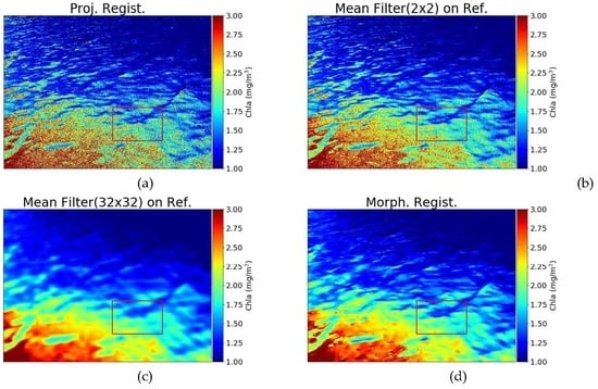
The results for the scene of much higher altitude (Scene-C (196 m)) are presented in Figure 16. It shows that the scene is in general more homogeneous than the previous low-altitude image (Scene-B (8.1 m)), and it exhibits a gradual radiance change across the scene with the boxed area occupied with fairly homogeneous radiance values. However, even if the surface features have a significantly smaller scale than the low-altitude images, the noisy pattern is still strong in all areas of the image as well as in the boxed area, which was effectively removed by the morphological band registration. In the boxed area, while the mean and the median values stay similar (mean: 2.248 to 2.229, media: 2.225 to 2.224), the scatter statics greatly improved (s.d.: 0.243 to 0.0066, c.v.: 11% to 3%) (Figure 16b). The proposed algorithm was also tested on a scene with an event in a part of the image (Figure 17). Scene-D was acquired for a strong red tide outbreak of Cochlodinium polykrikoides (the species was confirmed from microscopic analysis during the field campaign) and the Chla contents were estimated with the RBR algorithm. The morphological registration reduced the number of pixels that had extremely high Chla estimates (> 50 mg/m3), which are considered to be generated misregistration pixels. While the overall extent and concentration level in the morphological registration is comparable to that of the 32 × 32 filter results, a spatial pattern of a higher frequency is still observable in the improved result.
5. Discussion and Conclusions
This study analyzed the impact of residual misregistration between the bands of a multispectral camera, which is particularly problematic for fast-moving targets such as the water surface. The analysis suggested that the residual misregistration is difficult to correct using geometric coordinate transformation (e.g., projective transformation). It produces abnormal band ratios and band differences, resulting in significant anomalies in the water quality variables, such as the Chla concentration. The proposed registration algorithm succeeded in effectively removing noisy spatial patterns caused by the misregistration while maintaining the original spatial resolution of the image, unlike the smoothing approach which significantly degrades the sharpness of the images. Contrary to the intuition that high-altitude images will be less affected by pixel-level misregistration (because a scene appears more homogeneous when observed from far), the test results for various altitudes showed that the residual misregistration exist at all tested altitudes (8–390 m). This suggests that there exist various frequencies of the surface reflectance feature on the water surface. The proposed algorithm was robust to local events that occurred in a partial section of the image, which may have distinct spectral characteristics of the remaining image area (usually normal water surface), as shown in the red tide image.
The proposed method is expected to improve estimation of other water quality variables such as colored dissolved organic matter (CDOM) and total suspended sediments (TSM) as many of the CDOM and TSM retrieval algorithms rely on the band ratio of reflectance.
Future work includes analysis on the effects on other water quality variables, and also the further correction of residual sky reflectance that is often caused by the spatially varying normals of the wave facets. The residual sky reflectance still existed even after the morphological band registration. The research requires a comprehensive understanding of the reflecting mechanism and more detailed modeling of the surface reflectance, associated with the analysis on the downward sky radiance incident on the water surface.
Author Contributions
Data Curation, W.K., S.J. and Y.M.; Formal Analysis, W.K.; Validation, W.K.; Writing—Original draft, W.K.; Funding Acquisition, S.J.; Resources, S.J. and S.C.M.; Project Administration, Y.M.; Supervision, Y.M.; Writing—Review & editing, S.C.M. All authors have read and agreed to the published version of the manuscript.
Funding
Funding: This work was performed with the support of Jeollannam-do through the research project titled “Development of a monitoring system for damage reduction in aquacultures using marine environment observation drones” (B0080802000131) operated by the Jeonnam Technopark (JNTP), and was also supported by the National Research Foundation (NRF) project “Developing an atmospheric correction module for retrieving water quality from hyperspectral images” (NRF-2019R1F1A1062585).
Acknowledgments
The authors would like to thank Hyung-Jun Kim and Yoo-deok Boo for participating in the field campaign.
Conflicts of Interest
The authors declare no conflicts of interest
References
- Holtkamp, D.J.; Goshtasby, A.A. Precision registration and mosaicking of multicamera images. IEEE Trans. Geosci. Remote Sens. 2009, 47, 3446–3455. [Google Scholar] [CrossRef]
- Jhan, J.-P.; Rau, J.-Y.; Huang, C.-Y. Band-to-band registration and ortho-rectification of multilens/multispectral imagery: A case study of MiniMCA-12 acquired by a fixed-wing UAS. ISPRS J. Photogramm. Remote Sens. 2016, 114, 66–77. [Google Scholar] [CrossRef]
- Anuta, P.E. Spatial registration of multispectral and multitemporal digital imagery using fast Fourier transform techniques. IEEE Trans. Geosci. Electron. 1970, 8, 353–368. [Google Scholar] [CrossRef]
- D’Agostino, E.; Maes, F.; Vandermeulen, D.; Suetens, P. A Viscous Fluid Model for Multimodal Non-rigid Image Registration Using Mutual Information. Med. Image Anal. 2003, 7, 565–575. [Google Scholar] [CrossRef]
- Droske, M.; Rumpf, M. A Variational Approach to Nonrigid Morphological Image Registration. SIAM J. Appl. Math. 2004, 64, 668–687. [Google Scholar] [CrossRef] [Green Version]
- Matsopoulos, G.K.; Mouravliansky, N.A.; Delibasis, K.K.; Nikita, K.S. Automatic retinal image registration scheme using global optimization techniques. IEEE Trans. Inf. Technol. Biomed. 1999, 3, 47–60. [Google Scholar] [CrossRef] [PubMed]
- Soille, P. Morphological image compositing. IEEE Trans. Pattern Anal. Mach. Intell. 2006, 28, 673–683. [Google Scholar] [CrossRef]
- Tucker, C.J. Red and Photographic Infrared Linear Combinations for Monitoring Vegetation. Remote Sens. Environ. 1978, 8, 127–150. [Google Scholar]
- Huete, A.; Huete, A.R. A soil-adjusted vegetation index (SAVI). Remote Sens. Environ. 1988, 25, 295–309. [Google Scholar] [CrossRef]
- O’Reilly, J.E. Ocean color chlorophyll algorithms for Sea WiFS. J. Geophys. Res. Oceans 1998, 103, 24937–24953. [Google Scholar] [CrossRef] [Green Version]
- Siegel, D.A.; Wang, M.; Maritorena, S.; Robinson, W. Atmospheric correction of satellite ocean color imagery: The black pixel assumption. Appl. Opt. 2000, 39, 3582–3591. [Google Scholar] [CrossRef] [PubMed]
- Doxaran, D.; Froidefond, J.-M.; Castaing, P. A reflectance band ratio used to estimate suspended matter concentrations in sediment-dominated coastal waters. Int. J. Remote Sens. 2002, 23, 5079–5085. [Google Scholar] [CrossRef]
- Hu, C.; Carder, K.L.; Muller-Karger, F.E. Atmospheric correction of SeaWiFS imagery over turbid coastal waters: A practical method. Remote Sens. Environ. 2000, 74, 195–206. [Google Scholar] [CrossRef]
- Ruddick, K.G.; Ovidio, F.; Rijkeboer, M. Atmospheric correction of SeaWiFS imagery for turbid coastal and inland waters. Appl. Opt. 2000, 39, 897–912. [Google Scholar] [CrossRef] [PubMed] [Green Version]
- Kim, W.; Roh, S.-H.; Moon, Y.; Jung, S. Evaluation of Rededge-M Camera for Water Color Observation after Image Preprocessing. J. Korean Soc. Surv. Geod. Photogramm. Cartogr. 2019, 37, 167–175. [Google Scholar]
- Mueller, J.L.; Davis, C.; Arnone, R.; Frouin, R.; Carder, K.; Lee, Z.P.; Steward, R.G.; Hooker, S.; Mobley, C.D.; McLean, S.; et al. Above-water radiance and remote sensing reflectance measurements and analysis protocols. Ocean Opt. Protoc. Satell. Ocean Color Sens. Valid. Revis. 2000, 2, 98–107. [Google Scholar]
- Mobley, C.D. Estimation of the remote-sensing reflectance from above-surface measurements. Appl. Opt. 1999, 38, 7442–7455. [Google Scholar] [CrossRef] [PubMed]
- MicaSense GitHub. Available online: https://github.com/micasense/imageprocessing (accessed on 30 May 2020).
- Lee, Z.; Carder, K.L.; Mobley, C.D.; Steward, R.G.; Patch, J.S. Hyperspectral remote sensing for shallow waters I A semianalytical model. Appl. Opt. 1998, 37, 6329. [Google Scholar] [CrossRef] [PubMed]
- Lee, Z.; Ahn, Y.-H.; Mobley, C.; Arnone, R. Removal of surface-reflected light for the measurement of remote-sensing reflectance from an above-surface platform. Opt. Express 2010, 18, 26313–26324. [Google Scholar] [CrossRef] [PubMed]
- NASA. Ocean Biology Processing Group, Algorithm Theoretical Basis Documents for Chlorophyll-a Concentration Product. Available online: https://oceancolor.gsfc.nasa.gov/atbd/chlor_a/ (accessed on 30 May 2020).
- Noh, J.H.; Kim, W.; Son, S.H.; Ahn, J.-H.; Park, Y.-J. Remote quantification of Cochlodinium polykrikoides blooms occurring in the East Sea using geostationary ocean color imager (GOCI). Harmful Algae 2018, 73, 129–137. [Google Scholar] [CrossRef] [PubMed]
Figure 1.
A subset of a multispectral image acquired in a coastal area of Korea targeted on the ocean surface with normal states (low chlorophyll and suspended particle concentration), showing the differences in the spatial pattern for the five spectral bands.
Figure 1.
A subset of a multispectral image acquired in a coastal area of Korea targeted on the ocean surface with normal states (low chlorophyll and suspended particle concentration), showing the differences in the spatial pattern for the five spectral bands.

Figure 2.
(a) Lens configuration of Rededge-M camera and (b) the spectral response function of the bands overlaid with a typical vegetation spectrum (source: Rededge-M User Manual).
Figure 2.
(a) Lens configuration of Rededge-M camera and (b) the spectral response function of the bands overlaid with a typical vegetation spectrum (source: Rededge-M User Manual).

Figure 3.
(a) The map of study site near Yeosu, a southern coast of Korea, and the bounding box (orange) for the area that the unmanned aerial vehicle (UAV) was operated for, and (b) photographs of the multispectral-UAV system configured with the downwelling light sensor (DLS), the RGB camera, and the multispectral camera.

Figure 4.
Water reflectance image (RGB: Band 3, Band 2, Band 1) acquired by the Rededge-M for (a) Scene-A (85.4 m), (b) Scene-B (8.1 m), (c) Scene-C (196.2 m), and (d) Scene-D (390.5 m, red tide), with the UAV altitudes in the parenthesis.
Figure 4.
Water reflectance image (RGB: Band 3, Band 2, Band 1) acquired by the Rededge-M for (a) Scene-A (85.4 m), (b) Scene-B (8.1 m), (c) Scene-C (196.2 m), and (d) Scene-D (390.5 m, red tide), with the UAV altitudes in the parenthesis.

Figure 5.
Images of remote sensing reflectance (a,b) and the Chla estimates from the respective images (c,d) for Scene-A. A fixed Fresnel reflectance factor was applied to panel (a) and the adaptive approach was used for panel (b).
Figure 5.
Images of remote sensing reflectance (a,b) and the Chla estimates from the respective images (c,d) for Scene-A. A fixed Fresnel reflectance factor was applied to panel (a) and the adaptive approach was used for panel (b).

Figure 6.
Chla images for the subset area marked in Figure 5, with (a) the fixed and (b) the adaptive , and water reflectance images for Band 4 (c) and Band 5 (d).
Figure 6.
Chla images for the subset area marked in Figure 5, with (a) the fixed and (b) the adaptive , and water reflectance images for Band 4 (c) and Band 5 (d).

Figure 7.
(a) Regression results between the water reflectance for multispectral bands, with respect to Band 2, and (b) water reflectance for a 40 × 40 pixel subset area of Band 1, Band 1 estimates regressed from Band 2, the difference, and Chla estimates from the two bands.
Figure 7.
(a) Regression results between the water reflectance for multispectral bands, with respect to Band 2, and (b) water reflectance for a 40 × 40 pixel subset area of Band 1, Band 1 estimates regressed from Band 2, the difference, and Chla estimates from the two bands.

Figure 8.
The QQ plots of water reflectance for the four spectral bands, with respect to Band 2 and the corresponding regression results.
Figure 8.
The QQ plots of water reflectance for the four spectral bands, with respect to Band 2 and the corresponding regression results.

Figure 9.
Water reflectance of Band 1 for the subset area in Scene-A: (a) original data, (b) scaled from Band 2 through the location-based regression, and (c) scaled from Band 2 with the QQ-based regression.
Figure 9.
Water reflectance of Band 1 for the subset area in Scene-A: (a) original data, (b) scaled from Band 2 through the location-based regression, and (c) scaled from Band 2 with the QQ-based regression.

Figure 10.
Chla estimation from for the subset area in Scene-A: (a) original and (b) composited through the QQ-based regression.
Figure 10.
Chla estimation from for the subset area in Scene-A: (a) original and (b) composited through the QQ-based regression.

Figure 11.
Regression results for varying sizes of the QQ plot calculation window. The extent of each window is marked in the corrected Band 1 image.
Figure 11.
Regression results for varying sizes of the QQ plot calculation window. The extent of each window is marked in the corrected Band 1 image.

Figure 12.
Images of regression slopes (a) and y-intercepts (b) that are calculated at every pixel, and the slope images (c) and the y-intercept images (d) computed in every 12 pixels and convolved with a Gaussian filter.
Figure 12.
Images of regression slopes (a) and y-intercepts (b) that are calculated at every pixel, and the slope images (c) and the y-intercept images (d) computed in every 12 pixels and convolved with a Gaussian filter.

Figure 13.
The flow chart of the proposed algorithm.

Figure 14.
Comparison of resultant Chla estimates for Scene-A (altitude 85.4 m), before and after the application of the proposed morphological band registration method. Three subsections were magnified for improved visual evaluation.
Figure 14.
Comparison of resultant Chla estimates for Scene-A (altitude 85.4 m), before and after the application of the proposed morphological band registration method. Three subsections were magnified for improved visual evaluation.

Figure 15.
Scene-B, acquired on 2019.08.31 at an altitude of 8.1 m. (a) Chla estimates from four different processings of data; (upper left) before morphological registration, (upper right) after 2 × 2 mean filter on water reflectance, (bottom left) after 32 × 32 mean filter on water reflectance, and (bottom right) after morphological registration. (b) Magnified figures for the subset area marked in a red box in panel (a).

Figure 16.
Scene-C acquired on 2019.08.31 at an altitude of 196 m. (a) Chla estimates from four different processings of data; (upper left) before morphological registration, (upper right) after 2 × 2 mean filter on water reflectance, (bottom left) after 32 × 32 mean filter on water reflectance, and (bottom right) after morphological registration. (b) Magnified figures for the subset area marked in a red box in panel (a).

Figure 17.
Scene-D acquired on 2019.08.31 at an altitude of 390 m. (a) Chla estimates from four different processings of data; (upper left) before morphological registration, (upper right) after 2 × 2 mean filter on water reflectance, (bottom left) after 32 × 32 mean filter on water reflectance, and (bottom right) after morphological registration. (b) Close-up figures for the subset area marked in a red box in panel (a).


Table 1.
Data list used in this study.
| Scene ID | Time | Location | Altitude (m) | Scene Description |
|---|---|---|---|---|
| A | 26–07–2019 15:23 | Sumoon | 85.4 | Coastal Area |
| B | 31–08–2019 12:54 | Yeosu | 8.1 | From Ship |
| C | 31–08–2019 13:29 | Yeosu | 196 | Coastal Area |
| D | 31–08–2019 13:17 | Yeosu | 390 | Red Tide |
© 2020 by the authors. Licensee MDPI, Basel, Switzerland. This article is an open access article distributed under the terms and conditions of the Creative Commons Attribution (CC BY) license (http://creativecommons.org/licenses/by/4.0/).
Share and Cite
MDPI and ACS Style
Kim, W.; Jung, S.; Moon, Y.; Mangum, S.C. Morphological Band Registration of Multispectral Cameras for Water Quality Analysis with Unmanned Aerial Vehicle. Remote Sens. 2020, 12, 2024. https://doi.org/10.3390/rs12122024
AMA Style
Kim W, Jung S, Moon Y, Mangum SC. Morphological Band Registration of Multispectral Cameras for Water Quality Analysis with Unmanned Aerial Vehicle. Remote Sensing. 2020; 12(12):2024. https://doi.org/10.3390/rs12122024
Chicago/Turabian StyleKim, Wonkook, Sunghun Jung, Yongseon Moon, and Stephen C. Mangum. 2020. "Morphological Band Registration of Multispectral Cameras for Water Quality Analysis with Unmanned Aerial Vehicle" Remote Sensing 12, no. 12: 2024. https://doi.org/10.3390/rs12122024
Note that from the first issue of 2016, this journal uses article numbers instead of page numbers. See further details here.