The Impact of Artificial Wetland Expansion on Local Temperature in the Growing Season—the Case Study of the Sanjiang Plain, China


1
Northeast Institute of Geography and Agroecology, Chinese Academy of Sciences, Changchun 130012, China
2
College of Urban and Environmental Science, Changchun Normal University, Changchun 130032, China
*
Author to whom correspondence should be addressed.
Remote Sens. 2019, 11(24), 2915; https://doi.org/10.3390/rs11242915
Submission received: 12 October 2019
/
Revised: 1 December 2019
/
Accepted: 4 December 2019
/
Published: 5 December 2019
(This article belongs to the Special Issue Remote Sensing of Wetlands)
Abstract
:Land use and land cover change (LUCC) has been increasingly recognized as having important effects on climate systems. Paddy fields, one kind of artificial wetland, have seen a significant increase in the Sanjiang Plain, China since 2000 and have become the most typical LUCC at the regional scale. Against this background, in this paper, we discuss the effects of this artificial wetland increase on surface temperature, in addition to its driving mechanisms. Firstly, the spatiotemporal variations of land surface temperature (LST) and its two driving variables (albedo and latent heat flux (LE)) in the Sanjiang Plain are analyzed and assessed based on remote sensing observation information from 2001 to 2015. Our results from both spatial distribution difference and time series analysis show that paddy field expansion led to day-time cooling and night-time warming over the study area. However, the LST changes show different characteristics and magnitudes in the spring (May to June) compared to the other months of the growing season (July to September). The daytime cooling trend is found to be −0.3842 K/year and the warming trend at night 0.1988 K/year during the period 2001 to 2015, resulting in an overall cooling effect in May and June. In July–September, the LST changes have the same sign but a smaller magnitude, with a −0.0686 K/year temperature trend seen for the day-time and a 0.0569 K/year increase for the night-time. As a consequence, a pronounced decrease in the diurnal temperature range is detected in the growing season, especially in spring. Furthermore, albedo and LE are demonstrated to be very sensitive to land use changes, especially in the earlier periods of the growing season. Correlation analysis between LST and albedo and LE also indicates the dominant role played by evapotranspiration in paddy fields in regulating local temperature.
1. Introduction
Land use and land cover change (LUCC) plays an important role in regulating climate systems at different scales ranging from the global and regional to the local [1,2,3,4,5,6]. LUCC can alter land surface properties and subsequently influence surface heat and moisture in addition to greenhouse gas exchanges between the surface and atmosphere [7,8,9]. Although LUCC impacts on global climate based on different climate models were evaluated in the Intergovernmental Panel on Climate Change’s (IPCC’s) fifth assessment, the relative effects of biogeophysical feedback of LUCC on regional climate still lack comprehensive assessment [6,10]. Numerous studies have documented the spatiotemporally varied role that LUCC plays in modifying climate systems [5,11,12,13], among which deforestation and afforestation in different heat zones and different time periods is the most typical type of LUCC identified [14,15,16,17]. At the local to regional scale, which in the context of this paper was considered an area of 104 km2 or larger [18,19], the climate effects of LUCC in some typical areas may be considerably more significant than those at the global scale, and the magnitude of the effects can be similar to or even stronger than the climate change induced by greenhouse gases [8,20,21,22]. Meanwhile, different types of LUCC, such as urbanization, deforestation, desertification, irrigation, and wetland reclamation, can also contribute to different climate responses [23,24,25,26,27,28,29,30,31]. In this paper we focus mainly on the climatic effects of artificial wetland increase.
Containing the physical properties of both water and vegetation, wetlands have been regarded as cooling pools [32,33]. In contrast to urban areas wetlands redistribute more latent heat energy than sensible heat energy to the atmosphere and have cooling effects [27,34]. With higher evapotranspiration due to both water evaporation and vegetation canopy transpiration, wetlands are usually cooler than their surrounding drylands [35,36,37]. As a long-term natural change the magnitude of the cooling effects is similar to or even higher than the warming effects induced by urbanization [34,38]. Based on field observation, Bai’s study has shown the obvious cooling effects of wetlands on the ambient environment of the Zoige Plateau in China [33]. Gao et al. have documented the cold–humid effects of different kinds of wetlands in the Sanjiang Plain and found that the effects were closely related to the standing water depth and vegetation height [38]. Zhang et al. have demonstrated that the magnitude of cold–humid effects in wetlands is mainly influenced by vegetation type and wetland area [36,37,38]. However, although in situ station observation has the best reliability, it cannot cover continuous regions or illustrate spatial climate change patterns due to wetland changes [39]. Regional climate modeling is an effective and widely used approach employed to assess climate sensitivity due to wetland changes. Schneider and Eugster have simulated the climatic impacts of historical wetland drainage in Switzerland based on the “Lokal Modell” and found that wetland decrease can lead to different climatic characteristics and magnitudes in cold compared to warm seasons [40]. Guo’s study based on a regional climate model (RegCM) has shown that wetland shrinkage in the “Three-River Headwaters” of China brings less rainfall and warmer temperatures [41]. Thiery et al. have discussed the impact of African great lakes on regional climate and their results showed that the largest lakes cooled the annual near-surface air by 0.6 to 0.9 K on average [42]. Different regional climate models, parameter scheme selections, and representations of land surface may result, however, in varying responses to LUCC [7,43], which increases the uncertainty of the effects. It should be noted that remote sensing can provide a more direct method to evaluate the effects caused by local land use changes and their mechanisms [39,44].
Unlike slow wetland natural change, paddy field expansion, which involves a typical artificial wetland type, is in some regions rapid and substantial [45]. This short-term and abrupt land use change may bring about climate effects as important as those of urbanization at regional or local scales based on our previous studies [46,47], but this phenomenon lacks deep understanding and full attention. In the Sanjiang Plain in China, farmers tend to change their planting configuration from rainfed farmland to paddy fields instead of wetland reclamation because of national agriculture policy adjustments and ecological protection policies [7,48,49]. A large amount of paddy field expansion instead of wetland reclamation has become the main LUCC process since 2000 [45]. Hence, it is very important to understand climate responses to other rapid human-induced land use change that does not occur at the expense of destroying the ecological environment.
In this paper, based on remote sensing data, we first evaluate land surface temperature changes due to paddy expansion based on three methods and then analyze the corresponding changes of two critical land surface parameters or processes, albedo and latent heat flux (LE). Finally, we discuss the correlation between land surface temperature (LST) and albedo and LE and illustrate the driving mechanism of paddy field expansion in different growing seasons with regard to the local or regional climate. In summary, our study demonstrates the climatic effects of potential wetland restoration on regional climate, which will be helpful for wetland protection and recovery. Furthermore, our study provides new and direct evidence of the impact of short-term abrupt land use changes on regulating regional climate.
2. Materials and Methods
2.1. Study Area
The Sanjiang Plain, located in China’s north-east, extends from 45°01′00” N to 48°27’56” N in latitude and 130°13’00” E to 135°05’26” E in longitude. Previous studies have shown that the Sanjiang Plain has experienced significant land use changes since the 1950s, with a large area of marshes having been reclaimed into farmland over the past 60 years [27,45,47,50,51]. However, since 2000, because of a comparative income change, farmers have tended to cultivate rice instead of corn. As a result, conversion from rainfed farmland to paddy fields has become the main land use change, with this change able to lead to obvious climatic change at local and regional scales [27,47].
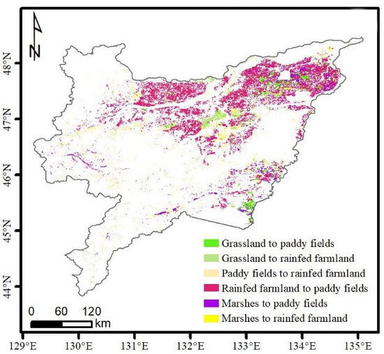
Land use distribution in 2001 and 2015 as shown in Figure 1 indicates that the land use pattern of the Sanjiang Plain was dominated by forest and farmland (including rainfed farmland and paddy fields). Land use maps for 2001 and 2015 were developed with human–computer interaction and interpretation based on Landsat 5 Thematic Mapper (TM) images for 2001 and Landsat 8 Operational Land Imager (OLI) images for 2015. The overall accuracy was 91.2% and the kappa index was 0.88 [47]. From 2001 to 2015, paddy fields increased from 1.28 × 10⁴ km2 (11.8% of the total area) to 2.85 × 10⁴ km2 (26.2% of the total area), with rainfed farmland decreasing from 4.0 × 10⁴ km2 (36.7% of the total area) to 3.37 × 10⁴ km2 (31.0% of the total area). The land use change map shown in Figure 1c also shows that paddy field expansion was the most obvious land use change during the period 2001 to 2015 within the Sanjiang Plain, for which expansion in rainfed farmland was dominant, followed by marshes and grassland. Considering the large area of marsh drainage here during the past century, this kind of land conversion is dramatic, and has had likely opposing effects on the climate. Corresponding land surface characteristic changes have made this area an effective case with which to study the impacts of land use change or land management adjustment on regional climate.
2.2. Data Processing and Method
In this study we mainly used remote sensing data to extract the direct influence of land use changes on LST as well as land surface albedo and latent heat flux LE, which are two of the most important parameters of the land–atmosphere process. The 8-day composite MOD11A2 Version 6 dataset was used to extract day-time and night-time LST values, which were named LSTD and LSTN, respectively [52]. We used the MCD43A3 Version 6 Albedo Model dataset to extract shortwave white sky albedo values for the study area [53]. The MOD16A2 Version 6 Evapotranspiration/Latent Heat Flux product was used to obtain LE values for the study area [54]. The spatial resolution of these datasets was resampled to 1 km. The composite time values for LST (LSTD and LSTN), albedo, and LE were aggregated to monthly means during 2001 to 2015. As the growing season in the Sanjiang Plain extends from May to September, we only extracted the data for this period when analyzing our results. Taking account of the typical physical properties of paddy fields, namely, that they are characterized by standing water in May and June, we divided the growing season into two periods: May and June, and July, August, and September. The following section will cover comparison and trend analyses for the two periods separately.
Based on land use data, pure rainfed farmland pixels and paddy field pixels, in addition to MODIS data at identical locations and resolutions, were extracted for each year from 2001 to 2015. In order to distinguish the LST differences between rainfed farmland and paddy fields, in addition to verifying the temperature change caused by paddy field expansion, two groups of these pixels were selected. Group A represented unchanged rainfed farmland (5730 pixels) and paddy fields (1575 pixels) during the period 2001 to 2015, while Group B represented paddy field pixels converted from rainfed farmland (2929 pixels). The locations of these pixels have been shown in Supplementary Materials Figure S1.
Influences of other anthropogenic and natural forces should be eliminated when studying regional or local climate change effects resulting from land use changes [40]. In our study, we used three approaches to evaluate the temperature responses due to paddy expansion from rainfed farmland:
- Regional statistical mean LST difference between rainfed farmland and paddy fields. The difference in LSTD and LSTN between rainfed farmland and paddy fields for each month (j) were calculated bywhere and are the day-time and night-time LST for the j-th month and i-th year for rainfed farmland in Group A, while and are the day-time and night-time LST for the j-th month and i-th year for paddy fields in Group A. n is equal to 15 and the i-th year represents years from 2001 to 2015.
- LST difference for the whole Sanjiang Plain between the end (2011–2015) and start (2001–2005) periods of our study period. Though this method involved climatology influences and interannual variation, it was the most intuitive way to illustrate the LST change corresponding to paddy field expansion. The albedo and LE changes were also obtained this way. Here, a t-test was used to verify the change significance of the LST, albedo, and LE for rainfed farmland, paddy fields, and change pixels between the two time periods.
- Time series analysis. Liu et al. (2019) have illustrated a warming trend in the Sanjiang Plain for the period the 1950s to 2015 [27]. To eliminate the impacts of climate warming, LST, albedo, and LE were rescaled to 0–1 before we conducted our time series analysis.where NVar is the rescaled variable, which was LST, albedo, or LE; is the variable value at pixel j; and and are the maximum and minimum values for the region at specific times, respectively. Then, an ordinary least square (OLS) regression was used to extract change trends for LST, albedo, and LE at each grid. The slope of the fitting function was calculated aswhere is the rescaled variable value for year i, n is equal to 15 in this study, and S is the slope for the changing tendency during the period 2001 to 2015. A value of S greater than 0 indicates an increasing trend, while a value less than 0 indicates a decreasing trend. Statistical tests based on a betainc t-test were conducted and only pixels with a significant change trend (p < 0.05) were illustrated and analyzed. The data processing was based on R software. Finally, the actual change trend for each variable was able to be formulated aswhere and are the regional maximum and minimum variable values, respectively, for the i-th year. The difference between S and Trend is that Trend is not dimensionless.
In the statistical analysis of the LST, albedo, and LE time series, the pixels of Group B, which represented paddy field expansion, were used to extract the change trend for each variable, while the pixels in Group A were used as verification.
3. Results
3.1. Impact of Land Use Change on LST, Albedo, and LE
Based on the 15-year time series LST data and the pixels of Group A, the regional average LST for rainfed farmland and paddy fields in the Sanjiang Plain was extracted. The monthly average LST differences between rainfed farmland and paddy fields, as well as the diurnal temperature ranges (DTRs) for rainfed farmland (DTR_R) and paddy fields (DTR_P) from 2001 to 2015, are shown in Table 1.
Throughout the entire growing season, the day-time LST in rainfed farmland can be seen to have been higher than that in paddy fields, while the night-time LST was the opposite. In comparison to the day-time LST difference between rainfed farmland and paddy fields, the magnitude of the night-time LST difference was smaller, contributing to overall cooler paddy fields and warmer rainfed farmland during the growing season. In May and June, the LSTD in rainfed farmland was 6.00 and 6.59 K higher than that in paddy fields, respectively, while the LSTN was 2.76 and 2.40 K cooler. As a result, the higher day-time temperature and cooler night-time temperature contributed to a larger diurnal temperature range for rainfed farmland than for paddy fields. In May and June, the DTR difference between the two farmlands was as high as 8–9 K. It also should be noted that the LST difference in August and September was not as obvious as that in May and June when standing water under the crops is most abundant.
To gain another perspective, we compared the spatial distribution of day-time LST and night-time LST between the periods 2011–2015 and 2001–2005 in the study area, as shown in Figure 2. The upper panels (Figure 2a,b,g,h) illustrate the LST for the period 2001–2005, the middle panels (Figure 2c,d,i,j) display the LST for the period 2011–2015, and the lower panels illustrate the LST changes during these two time periods. The left panels (Figure 2a–f) show the day-time LST and its changes while the right panels (Figure 2e–j) show the night-time LST and its changes. Figure 2a,c,e,g,i,k show the LST for the May–June period and Figure 2b,d,f,h,j,l shows the LST for the July–September period.
As we did not eliminate effects from the climate change background, the LST changes shown in Figure 2 involve effects from both land use changes and climate variations for the period 2001–2015. For the paddy field expansion areas, day-time LST in May and June in 2011–2015 was obviously cooler than that in 2001–2015 (Figure 2e), while night-time LST showed opposite warming effects (Figure 2k). From July to September, day-time LST in the farmland regions was cooler in 2011–2015 compared to that in 2001–2005, while it was warmer in the forest regions (Figure 2f). Night-time LST was consistently warmer in 2011–2015 (Figure 2l). Liu et al.’s (2018) study documented how temperature of the growing season during the period 2001–2015 displayed an increasing trend based on reanalysis data in the study area, which ignored climatic effects caused by land surface heterogeneity [47]. This suggests that effects from land use changes dominated land surface temperature changes in May and June and that climate disturbances may have been the main contributor to the land surface temperature increase during the period July to September.
Pixels of both Group A and Group B were used to extract LST changes for rainfed farmland and paddy fields in the Sanjiang Plain, as well as changes due to land use conversion from rainfed farmland to paddy fields, between the periods 2001–2005 and 2011–2015. The results are shown in Table 2.
It is not difficult to observe that conversion between the two cultivated strategies contributed to obvious LST changes. The statistical results show that day-time LST decreased 4.23 ± 1.64 K in May and June and 0.88 ± 0.83 K in July to September while night-time LST increased 3.92 ± 1.88 K in May and June and 1.75 ± 0.53 K in July to September. It should be noted that LST in unchanged cropland also showed some disturbances but this was not as significant as with the paddy expansion pixels. Climatology variation, vegetation cover fraction changes, and vegetation health condition changes, etc., could be reasons for the LST changes between these two time periods [40].
From another perspective, if we assume that the LST changes for the unchanged pixels represent the climate change background in this region while the LST changes for the changed pixels represent climate change due to both LUCC and the climate change background, we can estimate the contribution of LUCC to regional climate change. Generally, day-time LST change for unchanged cropland across the whole growing season was not significantly different from zero, indicating that the climate background in the day-time was relatively stable from 2001 to 2015. Night-time LST changes for unchanged cropland during the growing season showed a temperature increase of more than 1 K between the two time periods, indicating that, in the Sanjiang Plain, night-time temperature increase may be its dominant climate change characteristic. After separating the effects from the climate change background (the LST changes for the changed pixels minus the LST changes for the unchanged cropland pixels, including both rainfed farmland and paddy fields), the paddy expansion actually led to 3.84 K day-time cooling and 2.64 K night-time warming in May–June, which accounted for 91% and 67% of the LST change, respectively. In July–September, the magnitude of the LST responses due to LUCC was much smaller, i.e., 0.76 K day-time cooling and 0.67 K night-time warming, which contributed to 86% and 38% of the LST change, respectively.
3.2. Albedo and LE Responses under Different Land Use Patterns
At the regional scale, land use changes affect temperature mainly through biogeophysical processes [1]. Albedo and evapotranspiration (quantified by latent heat) are the critical parameters for radiation and non-radiation processes, respectively, through which land use changes ultimately influence climate systems [39,55]. Warming or cooling effects are decided by the counteraction between albedo–temperature feedback and the evapotranspiration process [43,56].
Albedo and LE for 2001–2005 and 2011–2015 are displayed in Figure 3. The changes in albedo and LE between the periods 2011–2015 and 2001–2005 reflect the impact of land use change on the two variables. The left panels (Figure 3a,b,c,d,e,f) show albedo across different years and seasons, as well as its changes across different time periods, while the right panels (Figure 3g,h,i,j,k,l) show LE. The upper panels display albedo (Figure 3a,b) and LE (Figure 3g,h) for 2001–2005, the middle panels display albedo (Figure 3c,d) and LE (Figure 3i,j) for 2011–2015, and the lower panels display albedo (Figure 3e,f) and LE (Figure 3k,l) changes between the two time periods. Figure 3a,c,e,g,i,k show the variables for May–June while Figure 3b,d,f,h,j,l show the variables for July–September.
Both albedo and LE showed different spatial distribution patterns for the periods 2001–2005 and 2011–2015. For the paddy field expansion areas, albedo changed from relatively high values to extremely low values in May and June, while in July to September, albedo showed a small, opposite-tending trend. Due to more standing water and a shorter vegetation canopy, the albedo of paddy fields was lower than that of rainfed farmland early in the growing season. However, when the plant height of corn exceeds that of rice, the vegetation canopy, rather than soil moisture, becomes the main restriction factor for albedo, and, as a result, albedo in some paddy fields was found to be even higher than that of rainfed farmland. By contrast, LE during the whole growing season showed a similar increasing trend between the periods 2011–2015 and 2001–2015. It is noteworthy that the regional spatial heterogeneity of LE in 2011–2015 showed a significant reduction compared with that for 2001–2005. The results suggest that the albedo changes seem to be more local and mainly focused on areas that have undergone land use change, while the LE changes are more regional, with effects not restricted only to areas of land use change but also their surrounding areas.
We used the pixels in Group A and Group B to detect albedo and LE changes between the periods 2011–2015 and 2001–2005. The results are shown in Table 3.
Conversion from rainfed farmland to paddy fields led to a 0.037 ± 0.013 albedo decrease in May and June and a 0.015 ± 0.008 increase in July to September, which was significantly different from that of both rainfed farmland and paddy fields themselves. The LE increased 0.016 ± 0.006 (108J/d/m2) in May and June and 0.010 ± 0.009 (108J/d/m2) in July to September due to paddy field expansion from rainfed farmland. Unchanged rainfed farmland and paddy fields also showed similar trends, but the magnitude was smaller. As expected, the results also indicated that albedo and LE changes were affected not only by land use changes but also climate changes and energy and water interactions between land surface and atmosphere at the regional scale.
Generally, albedo changes for the unchanged pixels showed a 0.007 decrease in May–June and a 0.011 increase in July–September, while LE changes showed increases of 0.014 × 10⁸ J/d/m2 and 0.008 × 10⁸ J/d/m2 in May–June and July–September, respectively. After separating the effects from the climate change background, paddy expansion actually led to a 0.03 albedo decrease in May–June and a 0.004 albedo increase in July–September which contributed to 81% and 27% of the overall albedo changes, respectively. LE changes due to LUCC were not as obvious as those of the albedo, which increased 0.002 × 10⁸ J/d/m2 during the growing season, and only account for 13% and 20% of the LE increase in May–June and July–September, respectively.
3.3. LST, Albedo and LE Change Trends During the Period 2001–2015
To eliminate the influence of climate disturbances, climatology variations, and data uncertainties on the results, we conducted a time series analysis based on normalized LST, albedo and LE for the period 2001–2015. The linear regression results are shown in Figure 4. The upper panels illustrate the change trend of day-time LST (Figure 4a,b), night-time LST (Figure 4c,d), albedo (Figure 4e,f) and LE (Figure 4g,h) over the study area for May–June and July–September, respectively, during the period 2001–2015. To avoid the influence due to mixed pixels, we used the pixels of Group B to extract the change trend of these variables caused by the land use conversion from rainfed farmland to paddy fields, as shown in the lower panels of Figure 4.
Generally, the change slopes for LST, albedo, and LE for May–June were much higher than those for July–September, indicating that the LST, albedo, and LE changes were concentrated in the former period of the growing season when the vegetation canopy was not big enough. In addition, more grids in May–June showed a significant change trend compared to those in July–September at a 95% level of confidence. Specifically, the regional average day-time LST decreased 0.09 K/year in May–June, with 34.6% of the total area changes being significant, out of which 89.6% of grids showed a decreased trend. The regional average night-time LST change trend in May–June was 0.04 K/year, with 44.5% of the total area showing significant changes, of which 50% of grids were mainly located in farmland areas showing an increasing trend and the other 50% mainly located in forest areas showing a decreasing trend. In July–September the significant grid proportion was much smaller compared to that in May–June, which was 21.7% and 24.1% for day-time and night-time LST changes, respectively. The May–June albedo decreased 0.00003/year during the period 2001–2015, with 52% of the Sanjiang Plain changing significantly, of which 47.3% decreased significantly, while the July–September albedo showed the opposite trend, with a 0.00008/year albedo increase for the whole region and 24.9% of grids changing significantly. The LE increased 0.04 MJ/d/m2/y across the whole growing season, with 50.0% and 23.5% of grids in the study area showing significant changes in May–June and July–September, respectively, and 88.0% and 92.4% of the significant grids showing an increasing trend.
Furthermore, the spatial distribution map of the change trend (Figure 4) suggests that the significant change trend area for LST, albedo, and LE was highly consistent with the areas where the rainfed farmland had been transformed into paddy fields. Specifically, 86.9% and 79.3% of the paddy field expansion pixels showed a significant day-time LST decrease in May–June and July–September, while 80.7% and 83.8% of the paddy field expansion pixels showed a significant night-time LST increase in May–June and July–September, respectively. Furthermore, 74.3% and 75.6% of the paddy field expansion pixels showed a significant LE increase in May–June and July–September, respectively, while 88.3% of the paddy field expansion pixels showed a significant albedo decrease in May–June and 77.8% of these pixels showed a significant albedo increase in July–September. The statistical analysis based on the pixels in Group B (the lower panels in Figure 4) illustrates that day-time LST had a cooling trend while night-time LST had a warming trend in both May–June and July–September. The day-time cooling trend was −0.3842 K/year and the warming trend at night was 0.1988 K/year, resulting in an overall cooling effect of about −0.0927 K/year in May and June. In July–September, the LST change showed the same sign but the magnitude was smaller, with a 0.0686 K/year temperature decreasing trend in the day-time and a 0.0569 K/year increase in the night-time, respectively. As a result, the DTR decreased significantly in the paddy field expansion areas.
We have also shown time series changes for two main parameters, albedo and LE, which dominate the radiation and non-radiation processes, respectively, that influence regional climate. Figure 4e,f illustrate the albedo change trend in May–June and July–September while Figure 4g,h shows the LE change trend in May–June and July–September, respectively. In contrast to the LST changes, the spatial pattern of albedo changes is quite different in May–June and July–September. In May–June, 52% of our study area showed significant albedo changes while only a small number of grids in July–September showed significant changes, especially for the paddy field expansion areas. The statistical results for the pure pixels indicated a consistent albedo decrease in May–June which was 0.0022/year, with R2 = 0.9265. Contrary to the albedo decrease in May–June, the albedo in July–September increased at a rate of 0.0005/year, which means that the albedo increase led to a cooling effect due to less absorbed solar radiation. LE throughout the whole growing season had an increasing trend for almost the whole region. The LE changes showed more regional characteristics compared with the local changes of LST and albedo. For the paddy field expansion pixels, the LE increased 0.1144 MJ/d/m2/year in May–June and 0.0803 MJ/d/m2/year in July–September, respectively.
3.4. Relationship between LST and Land Surface Parameters
From the above section, it is clear that there was good consistency between the LST changes and the albedo and LE changes. In this section, we discuss the relationship between LST and its driving factors. In the day-time, LST was mainly influenced by albedo and partitioning of surface energy, while night-time LST was more sensitive to heat capacity [7,57,58]. Irrigation in the paddy fields significantly increased the water content of soil across the whole growing season [46], which explains why the paddy fields were warmer than the rainfed farmland at night. However, the process was more complicated in the day-time because of the offset or accumulating impact of albedo and LE [44]. Thus, in this section we focus only on the relationship between day-time LST and albedo and LE. To make the results more convincing, we use rescaled day-time LST, albedo, and LE data in this section. The range of the three variables is between 0 and 1. The spatial distribution of correlation coefficients between day-time LST and albedo and LE is shown in the upper panel of Figure 5. The correlation analysis results for pixels of Group B, i.e., for conversion from rainfed farmland to paddy fields, are shown in the lower panel of Figure 5.
Spatial distributions of the correlation coefficients between day-time LST and albedo shown in Figure 5a indicate that 19.8% of the whole study area in May–June showed a significant correlation, 84.9% of which was positively correlated; 20.8% of the grids showed a significant correlation between day-time LST and LE and 91.4% were highly negatively correlated (Figure 5b). It should be noted that most of the highly correlated grids were located in paddy field expansion areas. Based on the energy balance equation, we can deduce that in May–June the LE played a dominant role in regulating LST and offset the effects from albedo changes. In July–September, the correlation between LST and both albedo and LE was not as significant as it was in May–June. Only 11.0% of the grids were significantly correlated between LST and albedo and 8.45% were significantly correlated between LST and LE (Figure 5c,d). In contrast to the positive correlation between LST and albedo in May–June, 72.4% of the significant grids showed a negative correlation, indicating the negative feedback between albedo and LST. This means that in July–September the albedo and LE had a synergy effect on LST.
The statistical analysis of the paddy expansion pixels (Figure 5e–h) illustrates that in May–June, day-time LST and albedo were highly positively related, while day-time LST and LE were highly negatively related, with R2 = 0.8273 and R2 = 0.4391, respectively, and both significant at the p < 0.05 significance level, indicating that low albedo and high LE corresponded to low day-time LST. With lower albedo, paddy fields tend to absorb more shortwave radiation, potentially leading to a warming effect. However, an overall cooling effect was observed in our results, suggesting that the net energy increase was counteracted by a greater latent heat loss and higher surface heat flux transport. This means that energy redistribution, rather than net radiation energy, plays a more important role in regulating local temperature, a finding which is in accordance with our previous works [27,46,47]. The higher correlation coefficient between day-time LST and albedo proves that albedo effects are more direct compared to those of LE [39].
In July–September the relationship between day-time LST and its two contributors was much weaker (R2 = 0.1942 and R2 = 0.028), but both showed negative correlation coefficients. Higher albedo in this period helps paddy fields reflect more energy and bring about a cooling effect; at the same time, more energy is transmitted to the atmosphere through latent heat and a cooling effect is also produced. Nevertheless, the accumulated cooling effects did not cause the day-time LST to be much cooler in July–September (Figure 4b) because of their low correlation and lesser significance.
4. Discussion
4.1. Advantages and Uncertainties of Detecting Regional Climate Responses Using Remote Seensing
Numerous observations and model simulations have detected the climate warming trend globally, particularly since 2000 [59]. However, global climate change has various driving factors and complicated geophysical and geochemical impact processes [7,60,61], and it is often difficult to distinguish these drivers from each other. Hence, evaluating climatic effects caused by land use changes without considering climatology changes can lead to significant uncertainties in results. In order to reduce this uncertainty, we used three evaluation methods based on remote sensing to illustrate and compare the impact of paddy field expansion on local surface temperature. The first method used multi-year regional average values to evaluate the LST difference due to LUCC, which eliminated the influences of climate fluctuation on the results; however, the results of this analysis could have been influenced by different geographic conditions such as latitude and elevation of each pure pixel and the distributions of the samples. As the Sanjiang Plain is a relatively small region with similar geographical properties, particularly for farmland, the first method proved to be effective in evaluating temperature responses. The second method avoided this limitation and detected LST changes for each LUCC pixel for the periods 2001–2005 and 2011–2015. However, this method involved effects from climate change. The third method rescaled the LST and comprised time series analysis for each grid pixel, which effectively eliminated the limitations described by the first two methods but with higher requirements for data quality. Through comparing the results from these three methods we can better understand the relationship between land use change, climate change, and climate response.
Compared with climate models, remote sensing has been proven to be a more effective and direct approach to generate local climatic effects due to land use changes [39,44]. Many previous studies have shown that the source of some limitations and uncertainties of model experiments originate from a lack of consistency in (1) the implementation of LUCC, (2) the representation of crop phenology, (3) the parameterization of albedo, and (4) the representation of evapotranspiration for different land cover types [43,62]. The MODIS data used in our study had relatively high spatial and temporal resolution, being a 1 km and 8-day or 16-day composite, and was able to generate good and consistent representation of LUCC, crop phenology, albedo, and vegetation and soil evapotranspiration, especially in long term monitoring. As remote sensing data are based on indirect methods of observation, the quality of the retrieval method may strongly influence the quality of assessments performed with these data. The MOD11 LST product is based on a combination of two algorithms; one of these algorithms retrieves both temperature and emissivity and the other uses prescribed values of emissivity to obtain temperature values [52]. Surface emissivity estimation is critical to LST retrieval and LUCC will definitely impact that emissivity. The emissivity in MOD11A2 was estimated by a classification-based emissivity method according to land cover types in the pixels determined by the input data in land cover (MCDLC1KM) and daily snow cover (MOD10_L2) [52]. However, the MCDLC1KM product does not distinguish paddy fields from rainfed farmland, which means conversion from rainfed farmland to paddy fields does not change emissivity significantly in MOD11A2 products. In reality, the increase in water content of the soil in paddy fields tends to increase the emissivity and, as a result, decrease the LST, which suggests that the estimated LST changes in this study may have some warming bias in the paddy field expansion areas. Similarly, the algorithms used to extract LE in MOD16A2 considered land cover to be one of the input elements [54], making it difficult to distinguish the spatial differences between rainfed farmland and paddy fields; this maybe one possible reason why LE showed less spatial heterogeneity between different croplands. Furthermore, although white sky albedo can reflect surface actual albedo properties [44], a lack of description of atmospheric conditions may add uncertainties to our results.
4.2. The Driving Mechanisms of Regional Temperature Change
It should be noted that in this paper we discuss LST responses caused by wetland increase and its two important driving factors, albedo and LE. As our previous studies have already documented how to use the energy balance to evaluate temperature effects and their corresponding contributors [27,47], in this paper we focused on direct temperature, albedo, and LE changes, in addition to their correlations, based on remote sensing, rather than describing the energy balance and exchanges. From our results, the land surface parameters albedo and latent heat flux showed corresponding changes due to paddy expansion, especially for the spring season. Many previous studies have demonstrated that both radiation and non-radiation processes ultimately determine temperature responses due to LUCC [7,14,43,56]. Albedo changes dominate total absorbed radiation energy, while evapotranspiration latent heat is the main factor of heat redistribution [7,55]. As a result, overall temperature effects result from the superposition of or counteraction between the two processes. Our results provided good examples of both radiation and non-radiation effects. Land surface temperature was positively correlated with albedo and negatively correlated with LE in spring and negatively correlated with both albedo and LE in summer. In spring, paddy fields were found to have lower albedo, which increased net radiation at the surface and should have increased the temperature; however, the significant increase in evapotranspiration consumed more energy than the net increase in radiation. This means that during May and June, evapotranspiration rather than albedo was the main driving factor for the temperature changes. For the summer season, increased albedo and LE improved the cooling effects. This conclusion is in agreement with our previous study, which discussed LST response mechanisms due to paddy expansion based on energy balance analysis [47]. However, our study showed inconsistent results with those of Schneider (2007) [41], who simulated historical wetland drainage in Switzerland and showed 0.1–0.2 °C cooling in the warm season, in which albedo increase played the dominant role. Compared with the table-based albedo change from the Schneider (2007) study, the magnitude of remote sensing-based albedo change between paddy fields and rainfed farmland in our study area was not excessively high, indicating that our results were more reliable than those using fixed table values, particularly for regional studies.
4.3. Future Research
Cold–humid effects from wetlands have been demonstrated via numerous field observations [32,33]. In this paper, we mainly focused on cold effects. However, our results also reflect the effects of humidity. Higher LE not only indicates that high latent heat was redistributed from the net surface radiation but also indicates that more soil moisture was transported to the atmosphere and, as a consequence, the humidity was increased [38]. From a water exchange prospective, Figure 3g–l and Figure 4g,h also suggest that paddy field expansion causes a larger scale latent heat increase in areas other than where wetland expansion has occurred. Paddy field irrigation in the earlier period of the growing season significantly increased the soil moisture, making it conducive for soil evaporation and vegetation transpiration and thereby enhancing water recycling [63]. These changes can lead to a different planetary boundary layer (PBL) structure, cloud cover regime, precipitation pattern, and other aspects of regional weather and climate [64,65,66,67,68]. Moreover, the transition zones of drylands and paddy fields can also help develop sea-breeze-like meso-scale circulations within the PBL and potentially promote convective cloud formation and precipitation in preferred areas [7]. This means that paddy field expansion may not only lead to temperature responses but also cause precipitation feedback, which will be further studied in our future works. Furthermore, in order to solve the problems of spatial heterogeneity mentioned in the results section, high resolution remote sensing datasets such as Sentinel imagery [69] can be used in our future works.
5. Conclusions
In our study, remote sensing observation information was used to detect LST changes and their driving mechanisms due to artificial wetland increase, namely, paddy field expansion. Our results from regional statistical average calculations, spatial distribution differences, and time series analysis showed that paddy field expansion led to day-time cooling and night-time warming over the study area. However, the LST changes showed different characteristics and magnitudes in the spring (May to June) compared to the other months of the growing season (July to September). Generally, the cooling effects were greater and more significant in the earlier period of the growing season. From regional statistical analysis we found that the daily LST in paddy fields was 1.62 and 2.10 K cooler than that of rainfed farmland in May and June, respectively, while in July–September, the LST difference between the two land use types was no more than 1 K. Meanwhile, the cooler day-time LST and warmer night-time LST contributed to decreased DTR in paddy fields, the magnitude of which reached 8–9 K. Time series analysis showed that because of paddy field expansion, the day-time cooling trend was −0.3842 K/year and the warming trend at night was 0.1988 K/year, resulting in an overall cooling effect of about −0.0927 K/year in May and June. In July–September, the LST change showed the same sign but the magnitude was much smaller, with a 0.0686 K/year temperature decreasing trend in the day-time and a 0.0569 K/year increase in the night-time. Furthermore, albedo and LE were demonstrated to be very sensitive to land use changes, especially in the earlier period of the growing season. Correlation analysis between LST and albedo and LE also indicated the dominant role that evapotranspiration in paddy fields plays in regulating local temperature. In summary, our study has provided good evidence that another instance of abrupt land use change, in addition to urbanization, will be able to profoundly affect local and regional climate. This study also suggests that land use management or land use adjustment can effectively influence regional climate patterns and can be used to provide advice and support for future land use planning, optimization, and regional sustainable development.
Supplementary Materials
The following are available online at https://www.mdpi.com/2072-4292/11/24/2915/s1, Figure S1: title: The locations of the pure pixels in Group A and Group B.
Author Contributions
Conceptualization, L.Y.; Methodology, L.Y.; Software, T.L.; Validation, T.L.; Formal analysis, T.L.; Investigation, L.Y.; Resources, L.Y.; Data curation, T.L.
Funding
This study was supported by the National Science and Technology basic resources survey project of China (2017FY101301), the National Natural Science Foundation of China (41601093 and 41701493), the Scientific and Technological Development Program of Jilin province (20180520096JH and 20190103152JH), and the program of the Northeast Institute of Geography and Agroecology, Chinese Academy of Sciences (IGA-135-05).
Acknowledgments
We thank the anonymous reviewers for their valuable and constructive comments.
Conflicts of Interest
The authors declare no conflict of interest.
References
- Foley, J.A.; DeFries, R.; Asner, G.P.; Barford, C.; Bonan, G.; Carpenter, S.R.; Chapin, F.S.; Coe, M.T.; Daily, G.C.; Gibbs, H.K.; et al. Global consequences of land use. Science 2005, 309, 570–574. [Google Scholar] [CrossRef] [PubMed] [Green Version]
- Mahmood, R.; Pielke, R.A.; Hubbard, K.G. Land use/land cover change and its impacts on climate. Glob. Planet Chang. 2006, 54, Vii. [Google Scholar] [CrossRef]
- Pielke, R.A.; Marland, G.; Betts, R.A.; Chase, T.N.; Eastman, J.L.; Niles, J.O.; Niyogi, D.D.S.; Running, S.W. The influence of land-use change and landscape dynamics on the climate system: Relevance to climate-change policy beyond the radiative effect of greenhouse gases. Philos. Trans. R. Soc. A 2002, 360, 1705–1719. [Google Scholar] [CrossRef] [PubMed]
- Kueppers, L.M.; Snyder, M.A.; Sloan, L.C.; Cayan, D.; Jin, J.; Kanamaru, H.; Kanamitsu, M.; Miller, N.L.; Tyree, M.; Due, H.; et al. Seasonal temperature responses to land-use change in the western United States. Glob. Planet Chang. 2008, 60, 250–264. [Google Scholar] [CrossRef]
- Brovkin, V.; Boysen, L.; Arora, V.K.; Boisier, J.P.; Cadule, P.; Chini, L.; Claussen, M.; Friedlingstein, P.; Gayler, V.; van den Hurk, B.J.J.M.; et al. Effect of Anthropogenic Land-Use and Land-Cover Changes on Climate and Land Carbon Storage in CMIP5 Projections for the Twenty-First Century. J. Clim. 2013, 26, 6859–6881. [Google Scholar] [CrossRef]
- Feddema, J.J.; Oleson, K.W.; Bonan, G.B.; Mearns, L.O.; Buja, L.E.; Meehl, G.A.; Washington, W.M. The importance of land-cover change in simulating future climates. Science 2005, 310, 1674–1678. [Google Scholar] [CrossRef] [Green Version]
- Mahmood, R.; Pielke, R.A.; Hubbard, K.G.; Niyogi, D.; Dirmeyer, P.A.; McAlpine, C.; Carleton, A.M.; Hale, R.; Gameda, S.; Beltran-Przekurat, A.; et al. Land cover changes and their biogeophysical effects on climate. Int. J. Climatol. 2014, 34, 929–953. [Google Scholar] [CrossRef]
- Bonan, G.B. Forests and climate change: Forcings, feedbacks, and the climate benefits of forests. Science 2008, 320, 1444–1449. [Google Scholar] [CrossRef] [Green Version]
- Dirmeyer, P.A.; Niyogi, D.; de Noblet-Ducoudre, N.; Dickinson, R.E.; Snyder, P.K. Impacts of land use change on climate. Int. J. Climatol. 2010, 30, 1905–1907. [Google Scholar] [CrossRef] [Green Version]
- Nuclear Regulatory Commission (NRC). Radiative Forcing of Climate Change: Expanding the Concept and Addressing Uncertainties; The National Academies Press: Washington, DC, USA, 2005; Volume 208. [Google Scholar]
- Li, Y.; De Noblet-Ducoudre, N.; Davin, E.L.; Motesharrei, S.; Zeng, N.; Li, S.C.; Kalnay, E. The role of spatial scale and background climate in the latitudinal temperature response to deforestation. Earth Syst. Dyn. 2016, 7, 167–181. [Google Scholar] [CrossRef] [Green Version]
- Nonomura, A.; Kitahara, M.; Masuda, T. Impact of land use and land cover changes on the ambient temperature in a middle scale city, Takamatsu, in Southwest Japan. J. Environ. Manag. 2009, 90, 3297–3304. [Google Scholar] [CrossRef] [PubMed]
- Fall, S.; Niyogi, D.; Gluhovsky, A.; Pielke, R.A.; Kalnay, E.; Rochon, G. Impacts of land use land cover on temperature trends over the continental United States: Assessment using the North American Regional Reanalysis. Int. J. Climatol. 2010, 30, 1980–1993. [Google Scholar] [CrossRef] [Green Version]
- Lee, X.; Goulden, M.L.; Hollinger, D.Y.; Barr, A.; Black, T.A.; Bohrer, G.; Bracho, R.; Drake, B.; Goldstein, A.; Gu, L.H.; et al. Observed increase in local cooling effect of deforestation at higher latitudes. Nature 2011, 479, 384–387. [Google Scholar] [CrossRef] [PubMed]
- Lejeune, Q.; Davin, E.L.; Guillod, B.P.; Seneviratne, S.I. Influence of Amazonian deforestation on the future evolution of regional surface fluxes, circulation, surface temperature and precipitation. Clim. Dyn. 2015, 44, 2769–2786. [Google Scholar] [CrossRef] [Green Version]
- Manoharan, V.S.; Welch, R.M.; Lawton, R.O. Impact of deforestation on regional surface temperatures and moisture in the Maya lowlands of Guatemala. Geophys. Res. Lett. 2009, 36. [Google Scholar] [CrossRef]
- Yu, L.X.; Zhang, S.W.; Tang, J.M.; Liu, T.X.; Bu, K.; Yan, F.Q.; Yang, C.B.; Yang, J.C. The effect of deforestation on the regional temperature in Northeastern China. Theor. Appl. Climatol. 2015, 120, 761–771. [Google Scholar] [CrossRef]
- Kustas, W.P.; Albertson, J.D.; Kustas, W.P.; Jackson, T.J.; Prueger, J.H.; Hatfield, J.L.; Anderson, M.C. Remote sensing field experiments evaluate retrieval algorithms and land-atmosphere modeling. EOS 2003, 84, 485–493. [Google Scholar] [CrossRef]
- Cleugh, H.A.; Raupach, M.R.; Briggs, P.R.; Coppin, P.A. Regional-scale heat and water vapour fluxes in an agricultural landscape: An evaluation of CBL budget methods at OASIS. Bound. Layer Meteorol. 2004, 110, 99–137. [Google Scholar] [CrossRef]
- Stohlgren, T.J.; Chase, T.N.; Pielke, R.A.; Kittel, T.G.F.; Baron, J.S. Evidence that local land use practices influence regional climate, vegetation, and stream flow patterns in adjacent natural areas. Glob. Chang. Biol. 1998, 4, 495–504. [Google Scholar] [CrossRef] [Green Version]
- Chase, T.N.; Pielke, R.A.; Kittel, T.G.F.; Zhao, M.; Pitman, A.J.; Running, S.W.; Nemani, R.R. Relative climatic effects of landcover change and elevated carbon dioxide combined with aerosols: A comparison of model results and observations. J. Geophys. Res. Atmos. 2001, 106, 31685–31691. [Google Scholar] [CrossRef] [Green Version]
- Avila, F.B.; Pitman, A.J.; Donat, M.G.; Alexander, L.V.; Abramowitz, G. Climate model simulated changes in temperature extremes due to land cover change. J. Geophys. Res. Atmos. 2012, 117. [Google Scholar] [CrossRef] [Green Version]
- Kalnay, E.; Cai, M. Impact of urbanization and land-use change on climate. Nature 2003, 423, 528–531. [Google Scholar] [CrossRef] [PubMed]
- Xue, Y.K. The impact of desertification in the Mongolian and the Inner Mongolian grassland on the regional climate. J. Clim. 1996, 9, 2173–2189. [Google Scholar] [CrossRef]
- Davin, E.L.; de Noblet-Ducoudré, N. Climatic Impact of Global-Scale Deforestation: Radiative versus Nonradiative Processes. J. Clim. 2010, 23, 97–112. [Google Scholar] [CrossRef]
- Kueppers, L.M.; Snyder, M.A.; Sloan, L.C. Irrigation cooling effect: Regional climate forcing by land-use change. Geophys. Res. Lett. 2007, 34. [Google Scholar] [CrossRef] [Green Version]
- Liu, T.X.; Yu, L.X.; Zhang, S.W. Impacts of Wetland Reclamation and Paddy Field Expansion on Observed Local Temperature Trends in the Sanjiang Plain of China. J. Geophys. Res. Earth 2019, 124, 414–426. [Google Scholar] [CrossRef]
- Puma, M.J.; Cook, B.I. Effects of irrigation on global climate during the 20th century. J. Geophys. Res. Atmos. 2010, 115. [Google Scholar] [CrossRef]
- Lim, Y.K.; Cai, M.; Kalnay, E.; Zhou, L.M. Observational evidence of sensitivity of surface climate changes to land types and urbanization. Geophys. Res. Lett. 2005, 32. [Google Scholar] [CrossRef] [Green Version]
- Mohan, M.; Kandya, A. Impact of urbanization and land-use/land-cover change on diurnal temperature range: A case study of tropical urban airshed of India using remote sensing data. Sci. Total Environ. 2015, 506, 453–465. [Google Scholar] [CrossRef]
- Ren, G.Y.; Zhou, Y.Q.; Chu, Z.Y.; Zhou, J.X.; Zhang, A.Y.; Guo, J.; Liu, X.F. Urbanization effects on observed surface air temperature trends in north China. J. Clim. 2008, 21, 1333–1348. [Google Scholar] [CrossRef] [Green Version]
- Yin, X.M.; Chen, W.W.; Gong, X.L.; Hong, W.; Wang, Y.Y. The cold-humid effect of perennially flooded marshes on clear days in the Sanjiang Plain of Northeast China. J. Food Agric. Environ. 2013, 11, 835–840. [Google Scholar]
- Xue, Z.S.; Hou, G.L.; Zhang, Z.S.; Lyu, X.G.; Jiang, M.; Zou, Y.C.; Shen, X.J.; Wang, J.; Liu, X.H. Quantifying the cooling-effects of urban and peri-urban wetlands using remote sensing data: Case study of cities of Northeast China. Landsc. Urban Plan. 2019, 182, 92–100. [Google Scholar] [CrossRef]
- Liu, Y.; Sheng, L.X.; Liu, J.P. Impact of wetland change on local climate in semi-arid zone of Northeast China. Chin. Geogr. Sci. 2015, 25, 309–320. [Google Scholar] [CrossRef] [Green Version]
- Muro, J.; Strauch, A.; Heinemann, S.; Steinbach, S.; Thonfeld, F.; Waske, B.; Diekkruger, B. Land surface temperature trends as indicator of land use changes in wetlands. Int. J. Appl. Earth Obs. 2018, 70, 62–71. [Google Scholar] [CrossRef]
- Gao, J.Q.; Lu, X.G.; Li, Z.F. Study on Cold-Humid Effects of Wetland in Sanjiang Plain. J. Soil Water Conserv. 2002, 16, 149–151. (In Chinese) [Google Scholar]
- Zhang, Y.; Lu, X.G.; Ni, J. Cold-humid ecological effects of the Sanjiang Plain. Ecol. Environ. 2004, 13, 37–39. (In Chinese) [Google Scholar]
- Bai, J.H.; Lu, Q.Q.; Zhao, Q.Q.; Wang, J.J.; Ouyang, H. Effects of Alpine Wetland Landscapes on Regional Climate on the Zoige Plateau of China. Adv. Meteorol. 2013, 2013. [Google Scholar] [CrossRef]
- Liang, S.L.; Wang, K.C.; Zhang, X.T.; Wild, M. Review on Estimation of Land Surface Radiation and Energy Budgets From Ground Measurement, Remote Sensing and Model Simulations. IEEE J. Stars 2010, 3, 225–240. [Google Scholar] [CrossRef]
- Schneider, N.; Eugster, W. Climatic impacts of historical wetland drainage in Switzerland. Clim. Chang. 2007, 80, 301–321. [Google Scholar] [CrossRef] [Green Version]
- Guo, A.H.; Wang, L.N.; Li, F.X. A Numerical Experiment Study of the Effects of Wetlands Shrinkage on Regional Climate in the ”Three-River Headwaters” Region. Clim. Environ. Res. 2010, 15, 743–755. (In Chinese) [Google Scholar]
- Thiery, W.; Davin, E.L.; Panitz, H.J.; Demuzere, M.; Lhermitte, S.; van Lipzig, N. The Impact of the African Great Lakes on the Regional Climate. J. Clim. 2015, 28, 4061–4085. [Google Scholar] [CrossRef]
- Pitman, A.J.; de Noblet-Ducoudré, N.; Cruz, F.T.; Davin, E.L.; Bonan, G.B.; Brovkin, V.; Claussen, M.; Delire, C.; Ganzeveld, L.; Gayler, V.; et al. Uncertainties in climate responses to past land cover change: First results from the LUCID intercomparison study. Geophys. Res. Lett. 2009, 36. [Google Scholar] [CrossRef] [Green Version]
- Peng, S.S.; Piao, S.L.; Zeng, Z.Z.; Ciais, P.; Zeng, H. Afforestation in china cools local land surface temperature. Proc. Natl. Acad. Sci. USA 2014, 111, 2915–2919. [Google Scholar] [CrossRef] [PubMed] [Green Version]
- Yan, F.Q.; Yu, L.X.; Yang, C.B.; Zhang, S.W. Paddy Field Expansion and Aggregation since the Mid-1950s in a Cold Region and Its Possible Causes. Remote Sens. (Basel) 2016, 10, 384. [Google Scholar] [CrossRef] [Green Version]
- Liu, T.X.; Yu, L.X.; Zhang, S.W. Land Surface Temperature Response to Irrigated Paddy Field Expansion: A Case Study of Semi-arid Western Jilin Province, China. Sci. Rep. UK 2019, 9. [Google Scholar] [CrossRef] [PubMed]
- Liu, T.X.; Yu, L.X.; Bu, K.; Yan, F.Q.; Zhang, S.W. Seasonal Local Temperature Responses to Paddy Field Expansion from Rain-Fed Farmland in the Cold and Humid Sanjiang Plain of China. Remote Sens. (Basel) 2018, 10, 2009. [Google Scholar] [CrossRef] [Green Version]
- Siebert, S.; Doll, P.; Hoogeveen, J.; Faures, J.M.; Frenken, K.; Feick, S. Development and validation of the global map of irrigation areas. Hydrol. Earth Syst. Sci. 2005, 9, 535–547. [Google Scholar] [CrossRef]
- Potter, P.; Ramankutty, N.; Bennett, E.M.; Donner, S.D. Characterizing the Spatial Patterns of Global Fertilizer Application and Manure Production. Earth Interact. 2010, 14. [Google Scholar] [CrossRef]
- Mao, D.H.; Wang, Z.M.; Wu, J.G.; Wu, B.F.; Zeng, Y.; Song, K.S.; Yi, K.P.; Luo, L. China’s wetlands loss to urban expansion. Land Degrad. Dev. 2018, 29, 2644–2657. [Google Scholar] [CrossRef]
- Mao, D.H.; Luo, L.; Wang, Z.M.; Wilson, M.C.; Zeng, Y.; Wu, B.F.; Wu, J.G. Conversions between natural wetlands and farmland in China: A multiscale geospatial analysis. Sci. Total Environ. 2018, 634, 550–560. [Google Scholar] [CrossRef]
- Wan, Z.; Hook, S.; Hulley, G. MOD11A2 MODIS/Terra Land Surface Temperature/Emissivity 8-Day L3 Global 1 km SIN Grid V006. 2015. Available online: https://doi.org/10.5067/MODIS/MOD11A2.006. (accessed on 12 November 2019).
- Schaaf, C.; Wang, Z. MCD43A3 MODIS/Terra+Aqua BRDF/Albedo Daily L3 Global-500 m V006. 2015. Available online: https://doi.org/10.5067/MODIS/MCD43A3.006. (accessed on 12 November 2019).
- Running, S.; Mu, Q.; Zhao, M. MOD16A2 MODIS/Terra Net Evapotranspiration 8-Day L4 Global 500m SIN Grid V006. 2017. Available online: https://doi.org/10.5067/MODIS/MOD16A2.006. (accessed on 12 November 2019).
- Liang, S.L.; Kustas, W.; Schaepman-Strub, G.; Li, X.W. Impacts of Climate Change and Land Use Changes on Land Surface Radiation and Energy Budgets. IEEE J. Stars 2010, 3, 219–224. [Google Scholar] [CrossRef] [Green Version]
- Bright, R.M.; Davin, E.; O’Halloran, T.; Pongratz, J.; Zhao, K.G.; Cescatti, A. Local temperature response to land cover and management change driven by non-radiative processes. Nat. Clim. Chang. 2017, 7, 296–305. [Google Scholar] [CrossRef]
- McNider, R.T.; Lapenta, W.M.; Biazar, A.P.; Jedlovec, G.J.; Suggs, R.J.; Pleim, J. Retrieval of model grid-scale heat capacity using geostationary satellite products. Part I: First case-study application. J. Appl. Meteorol. 2005, 44, 1346–1360. [Google Scholar] [CrossRef] [Green Version]
- Shi, X.Z.; McNider, R.T.; Singh, M.P.; England, D.E.; Friedman, M.J.; Lapenta, W.M.; Norris, W.B. On the behavior of the stable boundary layer and the role of initial conditions. Pure Appl. Geophys. 2005, 162, 1811–1829. [Google Scholar] [CrossRef]
- Intergovernmental Panel on Climate Change (IPCC). A simple method for reconstructing a high-quality NDVI time-series data set based on the Savitzky-Golay filter. Remote Sens. Environ. 2013, 91, 332–344. [Google Scholar] [CrossRef]
- Pongratz, J.; Reick, C.H.; Raddatz, T.; Claussen, M. Biogeophysical versus biogeochemical climate response to historical anthropogenic land cover change. Geophys. Res. Lett. 2010, 37. [Google Scholar] [CrossRef] [Green Version]
- Pinty, B.; Taberner, M.; Haemmerle, V.R.; Paradise, S.R.; Vermote, E.; Verstraete, M.M.; Gobron, N.; Widlowski, J.L. Biogeophysical effects of land use on climate: Model simulations of radiative forcing and large-scale temperature changes. J. Clim. 2011, 24, 4769. [Google Scholar] [CrossRef]
- Findell, K.L.; Pitman, A.J.; England, M.H.; Pegion, P.J. Regional and Global Impacts of Land Cover Change and Sea Surface Temperature Anomalies. J. Clim. 2009, 22, 3248–3269. [Google Scholar] [CrossRef]
- Pielke, R.A.; Adegoke, J.; Beltran-Przekurat, A.; Hiemstra, C.A.; Lin, J.; Nair, U.S.; Niyogi, D.; Nobis, T.E. An overview of regional land-use and land-cover impacts on rainfall. Tellus B 2007, 59, 587–601. [Google Scholar] [CrossRef]
- Pielke, R.A. Influence of the spatial distribution of vegetation and soils on the prediction of cumulus convective rainfall. Rev. Geophys. 2001, 39, 151–177. [Google Scholar] [CrossRef]
- Pielke, R.A.; Avissar, R. Influence of Landscape Structure on Local and Regional Climate. Landsc. Ecol. 1990, 4, 133–155. [Google Scholar] [CrossRef]
- Rabin, R.M.; Stadler, S.; Wetzel, P.J.; Stensrud, D.J.; Gregory, M. Observed Effects of Landscape Variability on Convective Clouds. Bull. Am. Meteorol. Soc. 1990, 71, 272–280. [Google Scholar] [CrossRef] [Green Version]
- Fu, C.B. Potential impacts of human-induced land cover change on East Asia monsoon. Glob. Planet Chang. 2003, 37, 219–229. [Google Scholar] [CrossRef]
- Wang, J.F.; Chagnon, F.J.F.; Williams, E.R.; Betts, A.K.; Renno, N.O.; Machado, L.A.T.; Bisht, G.; Knox, R.; Brase, R.L. Impact of deforestation in the Amazon basin on cloud climatology. Proc. Natl. Acad. Sci. USA 2009, 106, 3670–3674. [Google Scholar] [CrossRef] [Green Version]
- Jia, M.M.; Wang, Z.M.; Wang, C.; Mao, D.H.; Zhang, Y.Z. A New Vegetation Index to Detect Periodically Submerged Mangrove Forest Using Single-Tide Sentinel-2 Imagery. Remote Sens-Basel 2019, 11, 2043. [Google Scholar] [CrossRef] [Green Version]
Figure 1.
Land use maps of the Sanjiang Plain in 2001 (a) and 2015 (b), the main land use change types during the period 2001 to 2015 (c), and growing season temperature changes during the period 1951 to 2015 (d).
Figure 1.
Land use maps of the Sanjiang Plain in 2001 (a) and 2015 (b), the main land use change types during the period 2001 to 2015 (c), and growing season temperature changes during the period 1951 to 2015 (d).

Figure 2.
LST and LST changes within the Sanjiang Plain. (a) Day-time LST in May–June, 2001–2005; (b) day-time LST in July–September, 2001–2005; (c) day-time LST in May–June, 2011–2015; (d) day-time LST in July–September, 2011–2015; (e) day-time LST changes in May–June between the periods 2011–2015 and 2001–2005; (f) day-time LST changes in July–September between the periods 2011–2015 and 2001–2005; (g) night-time LST in May–June, 2001–2005; (h) night-time LST in July–September, 2001–2005; (i) night-time LST in May–June, 2011–2015; (j) night-time LST in July–September, 2011–2015; (k) night-time LST changes in May–June between the periods 2011–2015 and 2001–2005; (l) and night-time LST changes in July–September between the periods 2011–2015 and 2001–2005.

Figure 3.
Spatial distribution of albedo (ALB) and latent heat flux (LE) in the Sanjiang Plain. (a) ALB in May–June, 2001–2005; (b) ALB in July–September, 2001–2005; (c) ALB in May–June, 2011–2015; (d) ALB in July–September, 2011–2015; (e) ALB changes in May–June between the periods 2011–2015 and 2001–2005; (f) ALB changes in July–September between the periods 2011–2015 and 2001–2005; (g) LE in May–June, 2001–2005; (h) LE in July–September, 2001–2005; (i) LE in May–June, 2011–2015; (j) LE in July–September, 2011–2015; (k) LE changes in May–June between the periods 2011–2015 and 2001–2005; and (l) LE changes in July–September between the periods 2011–2015 and 2001–2005.

Figure 4.
Change trends for (a) day-time LST in May and June; (b) day-time LST in July to September; (c) night-time LST in May and June; (d) night-time LST in July to September; (e) albedo in May and June; (f) albedo in July to September; (g) LE in May and June; and (h) LE in July to September. Only grid points where the change trends are significant at a 95% level of confidence are shown. Linear regressions for the corresponding variables for the period 2001–2015 are shown in the lower panels and were calculated based on the pixels in Group B (** indicates the change trend is significant at p < 0.05).

Figure 5.
Spatial correlation coefficients between day-time LST and albedo in May–June (a) and July–September (c), and correlation coefficients between day-time LST and LE in May–June (b) and July–September (d) in the Sanjiang Plain. Only grid points significant at a 95% level of confidence are shown in these figures. (e–h) show the corresponding correlations for the paddy expansion pixels from Group B. ** indicates the correlation is significant at p < 0.05.


Table 1.
Land surface temperature (LST) and diurnal temperature range (DTR) differences between rainfed farmland and paddy fields (unit: K). Legend: LSTD, day-time LST; LSTN, night-time LST; DTR_R, DTR for rainfed farmland; DTR_P, DTR for paddy fields.
Table 1.
Land surface temperature (LST) and diurnal temperature range (DTR) differences between rainfed farmland and paddy fields (unit: K). Legend: LSTD, day-time LST; LSTN, night-time LST; DTR_R, DTR for rainfed farmland; DTR_P, DTR for paddy fields.
| Month | May | June | July | August | September |
|---|---|---|---|---|---|
| ∆LSTD | 6.00 | 6.59 | 2.69 | 0.99 | 1.55 |
| ∆LSTN | –2.76 | –2.40 | –1.00 | –0.74 | –0.26 |
| ∆LST | 1.62 | 2.10 | 0.85 | 0.13 | 0.65 |
| DTR_R | 21.35 | 17.69 | 9.27 | 8.09 | 12.10 |
| DTR_P | 12.58 | 8.69 | 5.58 | 6.36 | 10.29 |
∆ means the difference between rainfed farmland and paddy fields.
Table 2.
Day-time and night-time LST changes for the pixels in Group A and Group B between the periods 2011–2015 and 2001–2005.
Table 2.
Day-time and night-time LST changes for the pixels in Group A and Group B between the periods 2011–2015 and 2001–2005.
| Land Use State | Day-Time LST Changes in May–Jun | Night-Time LST Changes in May–Jun | Day-Time LST Changes in Jul–Sep | Night-Time LST Changes in Jul–Sep |
|---|---|---|---|---|
| Rainfed farmland | −0.46 ± 1.17 ** | 1.05 ± 0.42 ** | −0.78 ± 0.79 ** | 1.21 ± 0.29 ** |
| Paddy fields | −0.32 ± 1.12 | 1.51 ± 0.72 ** | 0.53 ± 0.49 | 0.96 ± 0.36 ** |
| Rainfed farmland Changes to paddy fields | −4.23 ± 1.64 ** | 3.92 ± 1.88 ** | −0.88 ± 0.83 ** | 1.75 ± 0.53 ** |
** indicates that LST changes are significant between 2011–2015 and 2001–2005 at p < 0.05; the value after ± is the root mean square error.
Table 3.
Albedo and LE changes between the periods 2011–2015 and 2001–2005 for pixels in Group A and Group B (** indicates that the albedo or LE changes for the conversion pixels are significantly different from both rainfed farmland and paddy fields at p < 0.05; the value after ± is the root mean square error).
| Land Use State | Albedo Changes in May–Jun | Albedo Changes in Jul–Sep | LE (108 J/d/m2) Changes in May–Jun | LE (108 J/d/m2) Changes in Jul–Sep |
|---|---|---|---|---|
| Rainfed farmland | −0.006 ± 0.008 ** | 0.011 ± 0.007 ** | 0.013 ± 0.006 ** | 0.013 ± 0.010 ** |
| Paddy fields | −0.008 ± 0.009 ** | 0.011 ± 0.008 ** | 0.015 ± 0.006 ** | 0.003 ± 0.009 ** |
| Rainfed farmland to paddy fields | −0.037 ± 0.013 ** | 0.015 ± 0.008 ** | 0.016 ± 0.006 ** | 0.010 ± 0.009 ** |
** indicates that albedo and LE changes are significant between 2011–2015 and 2001–2005 at p < 0.05; the value after ± is the root mean square error.
© 2019 by the authors. Licensee MDPI, Basel, Switzerland. This article is an open access article distributed under the terms and conditions of the Creative Commons Attribution (CC BY) license (http://creativecommons.org/licenses/by/4.0/).
Share and Cite
MDPI and ACS Style
Yu, L.; Liu, T. The Impact of Artificial Wetland Expansion on Local Temperature in the Growing Season—the Case Study of the Sanjiang Plain, China. Remote Sens. 2019, 11, 2915. https://doi.org/10.3390/rs11242915
AMA Style
Yu L, Liu T. The Impact of Artificial Wetland Expansion on Local Temperature in the Growing Season—the Case Study of the Sanjiang Plain, China. Remote Sensing. 2019; 11(24):2915. https://doi.org/10.3390/rs11242915
Chicago/Turabian StyleYu, Lingxue, and Tingxiang Liu. 2019. "The Impact of Artificial Wetland Expansion on Local Temperature in the Growing Season—the Case Study of the Sanjiang Plain, China" Remote Sensing 11, no. 24: 2915. https://doi.org/10.3390/rs11242915
Note that from the first issue of 2016, this journal uses article numbers instead of page numbers. See further details here.