Wetland Loss Identification and Evaluation Based on Landscape and Remote Sensing Indices in Xiong’an New Area
by
 , ,
, ,
Jinxia Lv
1,2 ,
,
Weiguo Jiang
1,2,*,
Wenjie Wang
3,
Zhifeng Wu
4,
Yinghui Liu
1,
Xiaoya Wang
1,2 and
Zhuo Li
1,2 1
State Key Laboratory of Earth Surface Processes and Resource Ecology, Faculty of Geographical Science, Beijing Normal University, Beijing 100875, China
2
State Key Laboratory of Remote Sensing Science, Faculty of Geographical Science, Beijing Normal University, Beijing 100875, China
3
Chinese Research Academy of Environmental Sciences, Beijing 100012, China
4
School of Geographical Science, Guangzhou University, Guangzhou 510006, China
*
Author to whom correspondence should be addressed.
Remote Sens. 2019, 11(23), 2834; https://doi.org/10.3390/rs11232834
Submission received: 5 October 2019
/
Revised: 25 November 2019
/
Accepted: 26 November 2019
/
Published: 29 November 2019
(This article belongs to the Special Issue Remote Sensing of Wetlands)
Abstract
:Wetlands play a critical role in the environment. With the impacts of climate change and human activities, wetlands have suffered severe droughts and the area declined. For the wetland restoration and management, it is necessary to conduct a comprehensive analysis of wetland loss. In this study, the Xiong’an New Area was selected as the study area. For this site, we built a new method to identify the patterns of wetland loss integrated the landscape variation and wetland elements loss based on seven land use maps and Landsat series images from the 1980s to 2015. The calculated results revealed the following: (1) From the 1980s to 2015, wetland area decreased by 40.94 km2, with a reduction of 13.84%. The wetland loss was divided into three sub stages: the wet stage from 1980s to 2000, the reduction stage from 2000 to 2019 and the recovering stage from 2009 to 2015. The wetland area was mainly replaced by cropland and built-up land, accounting for 98.22% in the overall loss. The maximum wetland area was 369.43 km2 in the Xiong’an New Area. (2) From 1989 to 2015, the normalized difference vegetation index (NDVI), normalized difference water index (NDWI) and soil moisture monitoring index (SMMI) showed a degradation, a slight improvement and degradation trend, respectively. The significantly degraded areas were 80.40 km2, 20.71 km2 and 80.05 km2 by the detection of the remote sensing indices, respectively. The wetland loss was mainly dominated by different elements in different periods. The water area (NDWI), soil moisture (SMMI) and vegetation (NDVI) caused the wetland loss in the three sub-periods (1980s–2000, 2000–2009 and 2009–2015). (3) According to the analysis in the landscape and elements, the wetland loss was summarized with three patterns. In the pattern 1, as water became scarce, the plants changed from aquatic to terrestrial species in sub-region G, which caused the wetland vegetation loss. In the pattern 2, due to the water area decrease in sub-regions B, C, D and E, the soil moisture decreased and then the aquatic plants grew up, which caused the wetland loss. In the pattern 3, in sub-region A, due to the reduction in water, terrestrial plants covered the region. The three patterns indicated the wetland loss process in the sub region scale. (4) The research integrated the landscape variation and element loss appears potential in the identification of the loss of wetland areas.
1. Introduction
Wetlands, formed in the transitional zone between land and water, are widely distributed worldwide [1]. These critical parts of ecosystems serve many essential functions to people and the environment, including supporting many wild animals and plant resources and providing flood protection, a water supply, erosion control and climate regulation [2,3,4]. However, with the development of urbanization and the population growth, global wetland areas have degraded or even disappeared [5], and the total wetland area in China is the fourth largest area of any country [6]. With the demand for ecological civilization, the wetland loss has received much attention from scientists.
Many researchers have attempted to identify wetland degradation. Current wetland degradation studies include wetland area degradation [7,8,9], wetland elements variation [10,11,12] and wetland ecosystem services [13]. The amount and pattern of wetland loss in China was analyzed from 1990 to 2010 based on land cover data [7]. The results showed that during these 20 years, China lost 2883 km2 of wetlands to urban expansion. Other researchers have reached similar conclusions. For instance, using Landsat images, wetland regions were extracted, which showed that China has experienced a net loss of 50,360 km2 from 1990 to 2000 [8]. In addition, using Landsat images, China’s wetlands loss was detected by the land use matrix and the results proposed that China’s total wetland area decreased by 101,399 km2 from 1978 to 2008 [9]. These studies mainly used the land use data to analyze the wetland loss and were concentrated on separate periods. They showed some deficiency in temporal continuity.
Due to the short-term nature of land use data availability, some researchers have analyzed wetland degradation based on the wetland elements by using long-term remote sensing data series. The critical wetland elements were water [10,14], vegetation [15,16] and soil moisture [14,17]. The water area variation of Wuhan urban agglomeration Lake was monitored with Landsat images [10]. The playa wetland condition was evaluated using four types of spectral water indices derived from Landsat images and the Google Earth Engine [14]. Furthermore, the wetland vegetation and soil moisture conditions were generally represented with the normalized difference vegetation index (NDVI) and the soil index to identify wetland change. For instance, the wetland vegetation was monitored in the Danshui River estuary in Taipei using the NDVI imagery produced from SPOT to monitor [18]. The Great Artesian Basin wetland vegetation was analyzed by using MODIS NDVI, and the results show that the vegetated wetland area declined from 2002 to 2009 [17]. The Biebrza Wetland soil moisture conditions were evaluated with the help of Sentinel-1 data [12]. Previous studies on wetland area analysis have focused on the wetland classes and have ignored the wetland area variation of the same class. Furthermore, studies of elements have concentrated on the evolution of a single element and have lacked a synthetic analysis. Therefore, it is necessary to establish a new method to identify the process of wetland loss by integrating the landscape with the elements succession process.
In China, there are many types of wetlands, including plateau, lake, coastal and urban wetlands [9]. Baiyangdian Lake, the largest natural freshwater wetland in the semi-arid North China Plain, is known as the “Pearl of North China” and the “Kidney of North China” and will be an important city wetland in the future of the Xiong’an New Area. On 1 April 2017, China’s Central Committee and State Council announced a plan to construct the Xiong’an New Area to improve the functioning of the non-capital in Beijing. In the future, the region will become an international metropolis. However, with the impact of climate change and human activities, the wetlands have suffered severe droughts and the wetland area has declined. Many efforts have been undertaken to identify the degradation and condition of wetlands [19,20,21]. For instance, it was analyzed that the long-term change in surface water area in the Xiong’an New Area using dense Landsat time series images, which indicated that the wetland has degraded and that this degradation was driven by human activities [20]. The ecological status of areas within the Xiong’an New Area was analyzed by proposing an ecological index [21]. This study is expected to build a new method for identifying wetland loss in the Xiong’an New Area and to shed light on wetland loss and future development.
The Xiong’an New Area was selected as the study area, with the purpose of proposing a new method for wetland loss identification. As increasing quantities of satellite data are becoming available, remote sensing data shows great importance in wetland field [22,23]. This study used Landsat time series images and seven land use datasets from 1989 to 2015 to analyze the wetland loss by the land cover transition matrix and trend analysis methods. Therefore, the specific objectives were (1) to analyze the wetland landscape variation and loss in the entire region and to calculate the maximum wetland area; (2) to evaluate the wetland elements loss in maximum wetland extent by sub-regions and (3) to summarize the pattern of wetland loss in the integrated landscape and elements and present a case study in wetland loss identification.
2. Materials
2.1. Study Area
The Xiong’an New Area has a sub-frigid and sub-humid climate, with an average annual temperature of approximately 12 °C. The Baiyangdian wetland, the largest freshwater wetland in North China, is located in the Xiong’an New Area and consists of more than 100 small and shallow lakes linked by numerous ditches. The region is located in Hebei Province of China, between 38.50–39.17°N and 115.58–116.42°E, which includes Xiong County, Anxin County, Rongcheng County and Gaoyang County in Baoding City and Renqiu City in Cangzhou City, and has an area of 2831.73 km2 and a population of 2.38 million [20]. The location of the Xiong’an New Area is shown in Figure 1. Annual precipitation varies widely from 400 to 500 mm, of which approximately 60% is received from June to September.
There are many lake shorelines in this region. According to the landforms and elevation differences, with reference to the water quality, current use and population density, seven functional zones named A, B, C, D, E, F and G were defined [24]. Sub-region A is dominated by beach and farmland, and the largest lake is Zaowandian. The water depth of sub-region B is 4 m, and it has a large lake named Shaochedian. Sub-region C includes some small lakes and the large lake of Lianhuadian. Sub-regions D and E include some lakes and provide many facilities for residents. Sub-region F includes some small lakes and the famous Baiyangdian. Sub-region G was seriously degraded, and the wetland was transformed to farmland.
2.2. Data Sources
The analysis was conducted using land use data and multi-date multi-temporal Landsat images from the sensors. Land use maps were developed in the late 1980s, 1995, 2000, 2005, 2007, 2009 and 2015 [25]. The land use maps for the Xiong’an New Area from the 1980s to 2015 is shown in Figure 2. The maps were acquired from the Institute of Geographic Sciences and Natural Resources Research, China (http://www.resdc.cn/), and have a spatial resolution of 30 m. The dataset analyses were conducted by a human-computer interactive interpretation method, using multi-date Landsat images. The accuracy of the six classes of land use was above 94.3%, which meets the requirement of the user mapping accuracy on the 1:100,000 scale. The wetlands were classified into seven types by the land use data, including paddies, rivers and canals, lakes, reservoirs and ponds, mud flats, beaches and marshes, and these classifications were used to address wetland landscape variation and loss processes in the spatial and temporal analyses.
Landsat images were the only data source applied to the method of wetland loss identification. During this study, Landsat images from 1989 to 2015 were acquired from the USGS (https://glovis.usgs.gov/) over a period of 27 years (Figure 3). We downloaded level 1 products with a cloud cover assessment threshold of 10%, for which the path/row numbers were 123/33. Twenty-seven scenes were used, including 22 scenes from the TM (1989–1999 and 2002–2012), two scenes from the ETM (2000–2001) and three scenes from the OLI (2013–2015). Most scenes clustered in the days 200 and 240, which were summer days. The images were used to calculate the wetland elements and to evaluate the loss of the wetland elements in the maximum wetland extent.
3. Methodology
3.1. The Analysis Method of Wetland Landscape Variation and Loss
3.1.1. Land Cover Transition Matrix
The wetland landscape variation was analyzed by the transfer probability matrix, which was proposed by Markov. The Markov pattern can be used to describe the changes in the structure and characteristics of land use types. This method not only shows the structure type of land use in two stages but also reflects the source and composition of each land use type in the study period [26]. The application of land use type conversion lies in the determination of the transition probability. The quantitative analysis of the conversion of wetland is conducted by the transfer of probability matrix, which could analyze the change of wetland area between different years. The mathematical expression is:
where P represents the area; n represents the number of types of land use; i and j represent the land use types at the beginning and the end of the study period, respectively and Pij is the transition probability from the ith class to the jth class.
3.1.2. Identifying the Maximum Wetland Extent
To better identify the wetland extent, we use seven land use maps to extract wetland areas. First, the maximum wetland was defined as it appeared in any period. Then, the wetland extent was analyzed by the overlay tools in ArcGIS 10.2 software. The spatial variation in wetlands extent was documented among the seven sub-regions. The elements in typical regions were chosen to analyze the succession process. The mathematical expression is:
where x represents the land use types; w represents the wetland types; k represents the number of the wetland maps and S represents the maximum wetland extent.
3.2. The Analysis Method of Wetland Elements Loss
3.2.1. Calculation of Wetland Elements
To make the pixel values comparable between images, all scenes were calibrated to the top of atmospheric (TOA) reflectance via radiometric calibration [10,27].
Water, vegetation and soil are the critical elements of a wetland, which play important roles in the maintenance of wetland function. In this study, the water element was indicated by the normalized difference water index (NDWI) [28]. The NDWI is expressed as:
where Green and NIR are the spectral reflectance values in the TM and ETM+ green and near infrared bands. This NDWI equation produces values in the range from −1 to 1, where positive values indicate water areas and negative values signify non-water surfaces.
The vegetation was indicated with the normalized difference vegetation index (NDVI) [29,30]. The NDVI is expressed as:
where NIR and Red are the spectral reflectance values in the TM and ETM+ near infrared and red bands. The NDVI values are in the same range as those of the NDWI.
The soil element was indicated by the soil moisture monitoring index (SMMI) [31], which indicates the bare land soil moisture (0–5 cm) and water conditions. The SMMI is expressed as:
where NIR and SWIR are the spectral reflectance in the TM and ETM+ near infrared and short wave infrared bands (1.55–1.75 um TM/ETM and 1.57–1.65 OLI).
NDWI, NDVI and SMMI maps were derived for all images from 1989 to 2015. Finally, the three indexes were used to evaluate the wetland elements loss in the maximum wetland extent.
3.2.2. Change Trend Analysis Method
The component was used for analyzing wetland elements dynamics to describe the variation trend. The NDVI, NDWI and SMMI (from 1989 to 2015) were investigated in the study area to analyze changes in the intra-annual trends. The Theil–Sen median trend analysis (TS), integrated with the Mann–Kendall test (MK) method, was the common tool employed for detecting changes.
Theil–Sen median trend analysis is a robust and non-parametric statistical trend calculation method, which can reduce the impacts of data anomalies. Theil–Sen median trend analysis was used to calculate the median of the slope of n × (n − 1)/2 data combinations, which was used to calculate each element change trend. Simultaneously, the MK test has been used to measure the degree to which a trend is consistently increasing or decreasing (with values ranging from −1 to +1) [32,33], and was recently employed for trend detection in an auto-correlated series. The time series of each element is from 1989 to 2015. The Z statistic values are as follows:
where and represent each element’s values in the ith and jth year, respectively; n represents the length of the time series and the statistic Z values range from (−∞, +∞). At a significance level of α (in this study, α = 0.05), if , then there is a significant change in the significance level.
Then, the change trends of the wetland elements were determined (Table 1). The element dynamics of water, vegetation and soil were analyzed in different periods. By analyzing the evolution of the element trends, we can determine the element succession processes and loss.
3.3. The Pattern of Wetland Loss in the Landscape Integrated with Elements
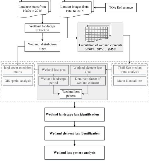
Under the impacts of climate and human activities, wetlands have been severely damaged, including the loss of external and internal wetland functions. Wetland landscape loss includes the encroachment of built-up land caused by reclamation and the conversion of wetlands to cropland for agricultural production. The loss is generally irreversible; irreversible loss is defined as the wetland loss caused by landscape variation. First, we used the land use transition matrix to analyze the wetland landscape change and loss from the spatial-temporal distributions of wetlands. Furthermore, the maximum wetland extent was defined in the Xiong’an New Area by GIS analysis. It is known that internal wetland changes are a result of the process of wetland elements loss in which water is reduced and vegetation is degraded. Then, we used the Theil–Sen median trend analysis (TS), integrated with the Mann–Kendall test (MK) method, to detect the wetland elements succession in the maximum wetland extent. Since each sub-region had different change trends in different periods, we proposed that the pattern of wetland loss in the Xiong’an New Area was integrated with the evolution of the wetland landscape and its elements (Figure 4).
4. Results
4.1. The Analysis of Wetland Landscape Variation and Loss
From the 1980s to 2015, the wetland landscape changed greatly in the Xiong’an New Area (Figure 5). In the Figure 5, each column of histogram represented the total transition probability of the certain land use type in year of 2015. Each portion of the column represented the transition probability from other land use types between the beginning to end of the period. From the 1980s to 2000, 26.54 km2 of wetlands recovered, which were transformed from cropland and represented 96.66% of the overall wetland recovery. During this period, the wetlands were in the wet stage. Between 2000 and 2009, 97.68 km2 of wetlands degraded, transforming into cropland and representing 90.12% of the overall wetland degradation. Wetland area had the largest reduction during this time, and this period is defined as the reduction stage. Additionally, the development of the land occupied by cropland and wetland increased continuously. Between 2009 and 2015, the wetland area was in the recovering stage and the wetland area increased by 30.20 km2 and was mainly transformed from croplands (92.42%). During these 30 years, built-up land increased continuously, mainly in the area occupied by cropland land, as well as in some land occupied by wetlands. The cropland transition was variable, and croplands changed both into wetlands and built-up lands.
Similarly, the spatial distribution of wetlands changed (Figure 6). During this period, the wetland area mainly showed a decreasing trend. From the 1980s to 2015, wetland area decreased by 40.94 km2, a reduction of 13.84%. Between the 1980s and 2000, the wetland area reached its maximum value in 1995. The increased wetland area was distributed in the southeast region. Between 2000 and 2009, 97.68 km2 of wetland mainly in the northwest and southeast of the region (sub-regions A and G) degraded and was transformed into farmland. Between 2009 and 2015, the wetland area was in a recovering stage and the wetland area increased by 30.20 km2. The increased area was distributed in the northwest region (sub-region A). In addition, the maximum wetland area was 369.43 km2 in the Xiong’an New Area.
The changed or disappeared regions were replaced with cropland and built-up land. In the past 30 years, 80.18 km2 (81.37%) of wetland area has been lost to cropland. In addition, 16.61 km2 of wetland area was lost to built-up land, representing 16.85% of the overall loss. A small amount of wetland area transformed into woodland (0.03 km2) and grassland (1.72 km2; Figure 7). We next analyzed the wetland elements succession processes in certain wetland extents.
4.2. The Wetland Elements Loss in the Maximum Wetland Extent
Severe drought occurred in the region in the mid-1980s (indicated by extremely low precipitation in 1986/1987), and heavy rainfall occurred in July to August of 1988. To make the wetland elements comparable at an annual scale, the time series were set from 1989 to 2015. In the maximum wetland extent, the vegetation, water and soil elements showed different variation trends from 1989 to 2015. As shown in Figure 8, the wetland elements showed different trends and the changes were divided into three periods. The NDVI showed a different trend from the NDWI, which illustrated that the vegetation and water changes were interdependent. The SMMI values were consistent with the landscape variation. According to the differences in element changes, the wetland elements loss could be explained from the different periods.
From 1989 to 2015, the NDVI showed a degrading trend and 272.99 km2 was degraded. The significantly degraded areas amounted to 80.40 km2, accounted for 19.84% of the entire area, and were distributed in sub-regions A, C, D and F. Furthermore, the NDWI showed a slightly increasing trend and the significantly increased areas amounted to 72.88 km2. The significantly degraded areas amounted to 20.71 km2 distributed in sub-region G and were transformed to farmland. The other sub-regions showed slight improvements or degradation and were distributed in a similar manner as the degraded area of the NDVI elements, which could be explained by the restraint of vegetation by indurated water. Moreover, the SMMI showed a degrading trend, and the significantly degraded areas amounted to 80.05 km2 distributed in the center of the lake (sub-regions C, D and F), as well as in some rivers. The variation in the different elements showed that different succession processes occurred in different sub-regions. From 1989 to 2015, sub-regions A, C, D and F were dominated by water inundation and the vegetation cover was restrained. However, the wetland soil moisture showed decreasing trends because the soil moisture was degraded and the water area had changed minimally. Sub-region G showed severe degradation, and its wetland areas were transformed into other land use types (Figure 9).
Under the influence of climate and human factors, the variation in wetland area occurred in three phases (1989–2000, 2000–2009 and 2009–2015). The wetland area was in a wet stage during 1989–2000 and a desiccation stage during 2000–2009. The process of succession of wetland elements was different in different periods (Figure 10).
The NDVI showed a slightly improving trend in the entire area from 1989 to 2000, and no significantly degraded area was created during this time period. Only a few patches in the middle of the Baiyangdian Lake displayed some degradation, which showed that the wetland vegetation was in good condition. From 2000 to 2009, the NDVI showed an improving trend, with a notable increase of 152.51 km2, showing that wetland vegetation was in a stable condition. Degradation occurred in some patches in sub-regions B, C, D, E and F. From 2009 to 2015, the variation trend was similar to that from the period (2000–2009) and the vegetation showed indications of being in a better condition. Furthermore, the area of significant improvement amounted to 266.91 km2, accounting for 67% of the entire area.
From 1989 to 2000, the NDWI showed a different trend than the NDVI. It showed a degrading trend, and the degraded areas amounted to 281.18 km2. The significantly degraded areas were distributed in sub-regions A, B and G. From 2000 to 2009, the NDWI showed a stable trend. From 2009 to 2015, the NDWI showed a degrading trend in the entire region and the significantly degraded area amounted to 90.02 km2. The degradation was distributed around the edges of Baiyangdian Lake.
From 1989 to 2000, the SMMI values demonstrated a slight decreasing trend but showed an increasing trend and an expansion in the spatial extent from 2000 to 2009. These regions were mainly distributed in sub-regions B, C, D and E. From 2009 to 2015, the SMMI showed a slightly increasing trend.
From 1989 to 2000, the wetland loss was dominated by water areas (NDWI), which were distributed in sub-regions A, B and G. These regions were degraded and replaced by terrestrial vegetation. The wetland area declined in this period. From 2000 to 2009, the wetlands were in a stable condition and the soil moisture (SMMI) showed a slightly degrading trend in sub-regions C, D and E. From 2009 to 2015, there was an overall upward trend in vegetation (NDVI) and the soil moisture (SMMI) showed a slight improvement. However, water in the edge areas was degraded, which could indicate that the aquatic vegetation occupied the water area. During the period, wetland area was recovered with the help of a water diversion project.
4.3. The Pattern of Wetland Loss in A Landscape Integrated with Elements
The wetland area that experienced degradation was analyzed using a transfer matrix, and the period was divided into three sections. In the wet period (from the 1980s to 2000), the wetland area was comparatively large and was dominated by lakes or reservoirs. From 2000 to 2009, the wetland area was in a reduction period. Some wetlands transformed into other land uses, and lakes were transformed into marshes, which indicated that wetland plants covered some of the water. Furthermore, from 2009 to 2015, the wetland area was in a recovering stage and the wetland area increased.
The region was divided into three parts according to the land use transitions present (Figure 11). The wetland area was occupied with impervious surfaces such as those of built-up lands and roads, which caused an irreversible loss of wetlands in the central region. In the southern region, the wetland was mainly transformed into croplands. In the northern region, the wetland area was degraded and then restored. However, the degraded wetland, except the land use change and the elements, changed. The process of wetland loss was summarized by different patterns integrated with the wetland area and elements.
The wetlands degraded due to the drought, and some wetlands were transformed into dry land or separated into small water fragments. Furthermore, some wetlands were able to recover with the help of artificial replenishment. Using the evolution of the wetland area and elements, we set up three change patterns and applied these patterns to the different sub-regions. In sub-region G, there was first a pattern of wetland loss (Figure 12). From 1989 to 2000, the water (NDWI) showed significant degradation. With the scarcity of water, aquatic plants grew. From 2000 to 2009, the vegetation (NDVI) showed a significant improvement. However, the mean value of NDVI decreased due to the presence of aquatic plants in the water, which indicated that aquatic plants were dominant. As the water gradually decreased, the vegetation changed from aquatic plants to terrestrial plants. From 2009 to 2015, the vegetation (NDVI) showed significant improvement and the mean value of NDVI increased. The terrestrial plants occupied sub-region G, and the wetland was transformed into cropland. The wetland area of sub-region G degraded completely.
The second pattern of wetland loss was represented in sub-regions B, C, D and E (Figure 13). From 1989 to 2000, the water area decreased, which resulted in a decrease in soil moisture. From 2000 to 2009, the soil moisture (SMMI) showed a slight degradation and the mean value of the SMMI decreased. Therefore, the aquatic plants were able to grow. From 2009 to 2015, the vegetation mainly improved. The sub-region was the critical area of the lake; therefore, the wetland existed in different forms. The wetland loss showed that the soil moisture degraded in the main extent and the aquatic plants and water were interdependent.
The third pattern of wetland loss was shown in sub-region A (Figure 14). This region experienced wetland loss in its early stage and wetland recovery in its late stage. From 1989 to 2000, the water (NDWI) showed a significant degradation and the mean value of NDWI decreased. The water area decreased during the period. From 2000 to 2009, due to the reduction in water, terrestrial plants covered the region. The vegetation (NDVI) showed significant improvement. However, the mean value of the NDVI gradually decreased. With the supplement of water, the wetland in sub-region A recovered. From 2009 to 2015, the aquatic plants occupied the area previously occupied by terrestrial plants. The vegetation (NDVI) showed significant improvement, and the mean value of the NDVI increased. Due to the supplement of water from the reservoir, the wetland area maintained its extent in a certain area.
5. Discussion
5.1. Contribution of the Wetland Loss Identification Method
Previous studies focused on determining wetland area change using land use data but neglected variations in the same water bodies. Wetland area would not change if the water level did not intensely change. The study conducted exploratory research to monitor wetland changes.
This paper identified wetland loss and summarized the patterns of wetland variation. First, the wetland loss was identified by the land use transfer matrix, which could extract the wetland loss area by transferring to other land use types (built-up land, farmland and grassland). The wetland area loss was unrecoverable in these regions. Then, the element trend analysis was conducted to indicate the wetland elements loss, which was used to complement the deficiency of wetland land use variation. The elements might explain the water, vegetation and soil characteristics from the continuous time series. Finally, we combined the land use loss and elements succession characteristics to summarize the different patterns of wetland loss in different periods. This method integrated the biological succession method and the GIS analysis method to evaluate wetland changes, which illustrates the spatial-temporal wetland changes from the continuous time series. Furthermore, this study could provide some guidance for wetland loss and recovery.
5.2. Comparison of the Wetland Loss
Compared with the previous studies in the Xiong’an New Area, the change in the trend of the wetland loss was mainly consistent. For instance, the long-term surface water area was analyzed in the Xiong’an New Area and the results showed that the water change was divided into three stages (late 1988 to late 1999, late 1999 to 2006 and 2007–2016) [20]. The water occupied the entire lake in the wet stage (water area = 360 km2). In this study, the wetland change was similarly divided into three stages (1989–2000, 2000–2009 and 2009–2015), and the largest wetland extent measured was 322.56 km2, which was 89.6% of that measured in the previous study. The Baiyangdian Lake area was measured, which changed from 81 km2 in 1974 to 47 km2 in 2007 using Landsat imagery. Additional studies have also shown declining trends from the 1950 to 2000s from gauge data collected at hydrological stations [19,34]. Most of these studies were based on satellite images or water level data, which provided an unparalleled record of the dynamic water surface.
5.3. Uncertainties and Prospects
Wetland loss identification is subject to complexity and uncertainty. First, wetland loss not only expresses the reduction in area but also is affected by the wetland function. The wetland loss identification method concentrated on the degradation of the wetland area and did not address other aspects of wetland variation. In further research, wetland structure and function would be included. Second, the wetland elements were analyzed from the Landsat images, and the remote sensing indices were sensitive to the season. Furthermore, the indices of water and vegetation were mutually affected. In further study the spatial and temporal resolution of the image should be more accurate, which could optimize the indices in some extent. Third, we summarized the three wetland loss patterns by integrating the landscape variation and element loss. According to the wetland loss pattern, we proposed some recommendations for the wetland restoration and management. In the northern region (sub region A), the condition of wetland vegetation is gradually restored, so the government should take more measures to maintain the wetland area. Furthermore, in the critical region (sub region B, C, D and E), the future plan needs to control the population and industrial scale to guarantee the core area. In the initial planning of the Xiong’an New Area, the region could establish a low impact development model and strengthen the construction of urban green infrastructure. In future studies, the Xiong’an New Area should expand the ecological source area and make more polices for wetland restoration and environment protection.
6. Conclusions
In this paper, wetland loss was analyzed from the landscape variation and wetland elements loss from the 1980s to 2015. Then, the different patterns of wetland loss were established by integrating the landscape with the elements in the Xiong’an New Area. From this, we learned that:
(1) From the 1980s to 2015, wetland area decreased by 40.94 km2, which was a reduction of 13.84%. This period of change was divided into three sub-periods (1980s–2000, 2000–2009 and 2009–2015), which were defined by their variation in wetland area as the wet stage, the reduction stage and the recovering stage. In the past 30 years, the loss of wetland area to cropland and built-up land was 80.18 km2 and 16.61 km2, respectively, which represents 81.37% and 16.85% of the overall loss. The northwest and southeast parts of the wetland region experienced great change, especially sub-region G. In addition, the maximum wetland area was 369.43 km2 in the Xiong’an New Area.
(2) From 1989 to 2015, the maximum wetland area derived from the NDVI, NDWI and SMMI indexes showed degradation, a slight increase and degradation trend, respectively. The significantly degraded areas were 80.40 km2, 20.71 km2 and 80.05 km2. The wetland area was dominated by different elements in different periods. From 1989 to 2000, the wetland loss was dominated by water area loss (NDWI), which was distributed in sub-regions A, B and G. From 2000 to 2009, the wetlands were in a stable condition and the soil moisture (SMMI) showed slight degradation in sub-regions C, D and E. From 2009 to 2015, there was an overall increase in vegetation (NDVI) and the soil moisture (SMMI) showed a slight improvement.
(3) The wetland loss was summarized by three patterns. The first pattern of loss occurred in sub-region G. With the scarcity of water, the NDWI indicated degradation, and then the aquatic plants were dominant. As the water gradually decreased, the vegetation changed from aquatic plants to terrestrial plants. Sub-region G degraded completely. The second pattern of wetland loss was represented by sub-regions B, C, D and E. The water area decreased, which caused the soil moisture (SMMI) to show a slight degradation, and then the aquatic plants grew. The aquatic plants and the water were interdependent, and the wetlands were in good condition in sub-regions B, C, D and E. The third pattern of wetland loss was displayed in sub-region A. As the water decreased, terrestrial plants covered the region. After water was supplemented, the wetland in sub-region A recovered. Aquatic plants replaced terrestrial plants, the vegetation (NDVI) showed a significant improvement and the mean value of NDVI increased.
Author Contributions
Data curation, J.L., X.W. and Z.L.; Funding acquisition, W.J.; Methodology, J.L.; Resources, Y.L.; Writing—original draft, J.L. and W.W.; Writing—review & editing, W.J. and Z.W.
Funding
This work was supported by the National Key Research and Development Program of China (2016YFC0503002), the National Natural Science Foundation of China (41571077) and the State Key Laboratory of Earth Surface Process and Resource Ecology (2017KF08).
Acknowledgments
Appreciation goes to the editors and reviewers for their valuable comments that have helped to improve this paper.
Conflicts of Interest
The authors declare that they have no conflict of interest.
References
- Li, S.; Wang, G.; Deng, W.; Hu, Y.; Hu, W.-W. Influence of hydrology process on wetland landscape pattern: A case study in the Yellow River Delta. Ecol. Eng. 2009, 35, 1719–1726. [Google Scholar] [CrossRef]
- Yu, H.; Zhang, F.; Johnson, V.C.; Bane, C.S.; Wang, J.; Ren, Y.; Zhang, Y. Analysis of land cover and landscape change patterns in Ebinur Lake Wetland National Nature Reserve, China from 1972 to 2013. Wetl. Ecol. Manag. 2017, 25, 619–637. [Google Scholar] [CrossRef]
- Yan, X.; Hu, Y.; Chang, Y.; Zhang, D.; Liu, M.; Guo, J.; Ren, B. Monitoring wetland changes both outside and inside reclamation areas for coastal management of the Northern Liaodong Bay, China. Wetlands 2017, 37, 885–897. [Google Scholar] [CrossRef]
- Hermoso, V.; Clavero, M.; Green, A.J. Dams: Keep wetland damage in check. Nature 2019, 568, 171. [Google Scholar] [CrossRef] [PubMed]
- Sica, Y.V.; Quintana, R.D.; Radeloff, V.C.; Gavier-Pizarro, G.I. Wetland loss due to land use change in the Lower Paraná River Delta, Argentina. Sci. Total Environ. 2016, 568, 967–978. [Google Scholar] [CrossRef] [PubMed]
- Zhou, D.; Gong, H.; Wang, Y.; Khan, S.; Zhao, K. Driving forces for the marsh wetland degradation in the Honghe National Nature Reserve in Sanjiang Plain, Northeast China. Environ. Model. Assess. 2009, 14, 101–111. [Google Scholar] [CrossRef]
- Mao, D.; Wang, Z.; Wu, J.; Wu, B.; Zeng, Y.; Song, K.; Yi, K.; Luo, L. China’s wetlands loss to urban expansion. Land Degrad. Dev. 2018, 29, 2644–2657. [Google Scholar] [CrossRef]
- Gong, P.; Niu, Z.; Cheng, X.; Zhao, K.; Zhou, D.; Guo, J.; Liang, L.; Wang, X.; Li, D.; Huang, H.; et al. China’s wetland change (1990–2000) determined by remote sensing. Sci. China Earth Sci. 2010, 53, 1036–1042. [Google Scholar] [CrossRef]
- Niu, Z. Mapping China’s wetlands and recent changes with remotely sensed data. In Remote Sensing of Wetlands; Tiner, R., Lang, M., Klemas, V., Eds.; CRC Press: Boca Raton, FL, USA, 2015; pp. 473–490. ISBN 978-1-4822-3735-1. [Google Scholar]
- Deng, Y.; Jiang, W.; Tang, Z.; Li, J.; Lv, J.; Chen, Z.; Jia, K. Spatio-temporal change of lake water extent in wuhan urban agglomeration based on landsat images from 1987 to 2015. Remote Sens. 2017, 9, 270. [Google Scholar] [CrossRef]
- Wang, X.; Wang, W.; Jiang, W.; Jia, K.; Rao, P.; Lv, J. Analysis of the Dynamic Changes of the Baiyangdian Lake Surface Based on a Complex Water Extraction Method. Water 2018, 10, 1616. [Google Scholar] [CrossRef]
- Dabrowska-Zielinska, K.; Budzynska, M.; Tomaszewska, M.; Malinska, A.; Gatkowska, M.; Bartold, M.; Malek, I. Assessment of carbon flux and soil moisture in wetlands applying Sentinel-1 Data. Remote Sens. 2016, 8, 756. [Google Scholar] [CrossRef]
- Clarkson, B.R.; Ausseil, A.-G.E.; Gerbeaux, P. Wetland ecosystem services. In Ecosystem Services in New Zealand: Conditions and Trends; Manaaki Whenua Press: Lincoln, New Zealand, 2013; pp. 192–202. [Google Scholar]
- Tang, Z.; Li, Y.; Gu, Y.; Jiang, W.; Xue, Y.; Hu, Q.; LaGrange, T.; Bishop, A.; Drahota, J.; Li, R. Assessing Nebraska playa wetland inundation status during 1985–2015 using Landsat data and Google Earth Engine. Environ. Monit. Assess. 2016, 188, 654. [Google Scholar] [CrossRef] [PubMed]
- Zhao, B.; Yan, Y.; Guo, H.; He, M.; Gu, Y.; Li, B. Monitoring rapid vegetation succession in estuarine wetland using time series MODIS-based indicators: An application in the Yangtze River Delta area. Ecol. Indic. 2009, 9, 346–356. [Google Scholar] [CrossRef]
- Petus, C.; Lewis, M.; White, D. Monitoring temporal dynamics of Great Artesian Basin wetland vegetation, Australia, using MODIS NDVI. Ecol. Indic. 2013, 34, 41–52. [Google Scholar] [CrossRef]
- Wu, C.; Chen, W.; Cao, C.; Tian, R.; Liu, D.; Bao, D. Diagnosis of wetland ecosystem health in the Zoige Wetland, Sichuan of China. Wetlands 2018, 38, 469–484. [Google Scholar] [CrossRef]
- Lee, T.-M.; Yeh, H.-C. Applying remote sensing techniques to monitor shifting wetland vegetation: A case study of Danshui River estuary mangrove communities, Taiwan. Ecol. Eng. 2009, 35, 487–496. [Google Scholar] [CrossRef]
- Hu, S.; Liu, C.; Zheng, H.; Wang, Z.; Yu, J. Assessing the impacts of climate variability and human activities on streamflow in the water source area of Baiyangdian Lake. J. Geogr. Sci. 2012, 22, 895–905. [Google Scholar] [CrossRef]
- Song, C.; Ke, L.; Pan, H.; Zhan, S.; Liu, K.; Ma, R. Long-term surface water changes and driving cause in Xiong’an, China: From dense Landsat time series images and synthetic analysis. Sci. Bull. 2018, 63, 708–716. [Google Scholar] [CrossRef]
- Xu, H.; Wang, M.; Shi, T.; Guan, H.; Fang, C.; Lin, Z. Prediction of ecological effects of potential population and impervious surface increases using a remote sensing based ecological index (RSEI). Ecol. Indic. 2018, 93, 730–740. [Google Scholar] [CrossRef]
- Szantoi, Z.; Brink, A.; Buchanan, G.; Bastin, L.; Lupi, A.; Simonetti, D.; Mayaux, P.; Peedell, S.; Davy, J. A simple remote sensing based information system for monitoring sites of conservation importance. Remote Sens. Ecol. Conserv. 2016, 2, 16–24. [Google Scholar] [CrossRef]
- Jia, M.; Wang, Z.; Wang, C.; Mao, D.; Zhang, Y. A New vegetation index to detect periodically submerged mangrove forest using single-tide sentinel-2 imagery. Remote Sens. 2019, 11, 2043. [Google Scholar] [CrossRef]
- Zhao, Y.; Zhang, X.; Ma, D.; Zhang, Y. Baiyangdian functional area division principle. Chin. J. Environ. Sci. 1995, S1, 41–44. [Google Scholar]
- Liu, J.; Kuang, W.; Zhang, Z.; Xu, X.; Qin, Y.; Ning, J.; Zhou, W.; Zhang, S.; Li, R.; Yan, C. Spatiotemporal characteristics, patterns, and causes of land-use changes in China since the late 1980s. J. Geogr. Sci. 2014, 24, 195–210. [Google Scholar] [CrossRef]
- Wan, L.; Zhang, Y.; Zhang, X.; Qi, S.; Na, X. Comparison of land use/land cover change and landscape patterns in Honghe National Nature Reserve and the surrounding Jiansanjiang Region, China. Ecol. Indic. 2015, 51, 205–214. [Google Scholar] [CrossRef]
- Jia, K.; Jiang, W.; Li, J.; Tang, Z. Spectral matching based on discrete particle swarm optimization: A new method for terrestrial water body extraction using multi-temporal Landsat 8 images. Remote Sens. Environ. 2018, 209, 1–18. [Google Scholar] [CrossRef]
- McFeeters, S.K. The use of the Normalized Difference Water Index (NDWI) in the delineation of open water features. Int. J. Remote Sens. 1996, 17, 1425–1432. [Google Scholar] [CrossRef]
- Yuan, F.; Bauer, M.E. Comparison of impervious surface area and normalized difference vegetation index as indicators of surface urban heat island effects in Landsat imagery. Remote Sens. Environ. 2007, 106, 375–386. [Google Scholar] [CrossRef]
- Ke, Y.; Im, J.; Lee, J.; Gong, H.; Ryu, Y. Characteristics of Landsat 8 OLI-derived NDVI by comparison with multiple satellite sensors and in-situ observations. Remote Sens. Environ. 2015, 164, 298–313. [Google Scholar] [CrossRef]
- Liu, Y.; Ma, W.; Yue, H.; Zhao, H. Dynamic soil moisture monitoring in shendong mining area using Temperature Vegetation Dryness Index. In Proceedings of the 2011 International Conference on Remote Sensing, Environment and Transportation Engineering (RSETE), Nanjing, China, 24–26 June 2011; IEEE: Piscataway, NJ, USA, 2011; pp. 5892–5895. [Google Scholar]
- Kendall, M.G. A new measure of rank correlation. Biometrika 1938, 30, 81–93. [Google Scholar] [CrossRef]
- Jiang, W.; Yuan, L.; Wang, W.; Cao, R.; Zhang, Y.; Shen, W. Spatio-temporal analysis of vegetation variation in the Yellow River Basin. Ecol. Indic. 2015, 51, 117–126. [Google Scholar] [CrossRef]
- Moiwo, J.P.; Yang, Y.; Li, H.; Han, S.; Yang, Y. Impact of water resource exploitation on the hydrology and water storage in Baiyangdian Lake. Hydrol. Process. 2010, 24, 3026–3039. [Google Scholar] [CrossRef]
Figure 1.
Location of the Xiong’an New Area and the land use map for 2015.

Figure 2.
Land use maps for the Xiong’an New Area from the 1980s to 2015.

Figure 3.
The data sources of Landsat images.

Figure 4.
The schematic diagram of the pattern of wetland loss.

Figure 5.
Land use type transition probability in the Xiong’an New Area.

Figure 6.
The spatial change maps of wetlands and the maximum wetland extent in the Xiong’an New Area.
Figure 6.
The spatial change maps of wetlands and the maximum wetland extent in the Xiong’an New Area.

Figure 7.
Landscape variation in wetland loss from the 1980s to 2015.

Figure 8.
The change maps of the mean values of the normalized difference vegetation index (NDVI), normalized difference water index (NDWI) and soil moisture monitoring index (SMMI) in the sub-regions.
Figure 8.
The change maps of the mean values of the normalized difference vegetation index (NDVI), normalized difference water index (NDWI) and soil moisture monitoring index (SMMI) in the sub-regions.

Figure 9.
Wetland element dynamic analysis from 1989 to 2015.

Figure 10.
Wetland element dynamic analysis in different periods.

Figure 11.
The wetland loss map (a1, b1 and c1 represent the land use map in the 1980s; a2, b2 and c2 represent the land use map in 2015).
Figure 11.
The wetland loss map (a1, b1 and c1 represent the land use map in the 1980s; a2, b2 and c2 represent the land use map in 2015).

Figure 12.
The first pattern of wetland loss (with the scarcity of water, aquatic plants were dominant and then transitioned to terrestrial plants).
Figure 12.
The first pattern of wetland loss (with the scarcity of water, aquatic plants were dominant and then transitioned to terrestrial plants).

Figure 13.
The second pattern of wetland loss (as the water area was reduced, the soil moisture decreased. Then, the aquatic plant grows up).
Figure 13.
The second pattern of wetland loss (as the water area was reduced, the soil moisture decreased. Then, the aquatic plant grows up).

Figure 14.
The third pattern of wetland loss (due to the reduction in water, terrestrial plants covered the region. With the supplement of water, aquatic plants recovered and took over the area previously occupied by the terrestrial plants).
Figure 14.
The third pattern of wetland loss (due to the reduction in water, terrestrial plants covered the region. With the supplement of water, aquatic plants recovered and took over the area previously occupied by the terrestrial plants).


Table 1.
The change trends of the wetland elements.
| SNDVI | SNDWI | SSMMI | Z Value | Trend of the Wetland Element |
|---|---|---|---|---|
| ≥0.005 | ≥0 | ≥0 | ≥1.96 | Significant degradation |
| ≥0.005 | ≥0 | ≥0 | −1.96–1.96 | Slight degradation |
| −0.005–0.005 | — | — | −1.96–1.96 | Stability |
| <−0.005 | <0 | <0 | −1.96–1.96 | Slight improvement |
| <−0.005 | <0 | <0 | <−1.96 | Significant improvement |
For the few pixel numbers where (−0.005 < SNDVI < 0.005, Z > 1.96 or Z < −1.96), pixels were defined as stable.
© 2019 by the authors. Licensee MDPI, Basel, Switzerland. This article is an open access article distributed under the terms and conditions of the Creative Commons Attribution (CC BY) license (http://creativecommons.org/licenses/by/4.0/).
Share and Cite
MDPI and ACS Style
Lv, J.; Jiang, W.; Wang, W.; Wu, Z.; Liu, Y.; Wang, X.; Li, Z. Wetland Loss Identification and Evaluation Based on Landscape and Remote Sensing Indices in Xiong’an New Area. Remote Sens. 2019, 11, 2834. https://doi.org/10.3390/rs11232834
AMA Style
Lv J, Jiang W, Wang W, Wu Z, Liu Y, Wang X, Li Z. Wetland Loss Identification and Evaluation Based on Landscape and Remote Sensing Indices in Xiong’an New Area. Remote Sensing. 2019; 11(23):2834. https://doi.org/10.3390/rs11232834
Chicago/Turabian StyleLv, Jinxia, Weiguo Jiang, Wenjie Wang, Zhifeng Wu, Yinghui Liu, Xiaoya Wang, and Zhuo Li. 2019. "Wetland Loss Identification and Evaluation Based on Landscape and Remote Sensing Indices in Xiong’an New Area" Remote Sensing 11, no. 23: 2834. https://doi.org/10.3390/rs11232834
Note that from the first issue of 2016, this journal uses article numbers instead of page numbers. See further details here.