Past and Future Trajectories of Farmland Loss Due to Rapid Urbanization Using Landsat Imagery and the Markov-CA Model: A Case Study of Delhi, India

Center for Spatial Information Science and Systems, George Mason University, 4087 University Drive, Fairfax, VA 22030, USA
*
Author to whom correspondence should be addressed.
Remote Sens. 2019, 11(2), 180; https://doi.org/10.3390/rs11020180
Submission received: 10 December 2018
/
Revised: 10 January 2019
/
Accepted: 15 January 2019
/
Published: 18 January 2019
(This article belongs to the Special Issue Selected Papers from Agro-Geoinformatics 2018)
Abstract
:This study integrated multi-temporal Landsat images, the Markov-Cellular Automation (CA) model, and socioeconomic factors to analyze the historical and future farmland loss in the Delhi metropolitan area, one of the most rapidly urbanized areas in the world. Accordingly, the major objectives of this study were: (1) to classify the land use and land cover (LULC) map using multi-temporal Landsat images from 1994 to 2014; (2) to develop and calibrate the Markov-CA model based on the Markov transition probabilities of LULC classes, the CA diffusion factor, and other ancillary factors; and (3) to analyze and compare the past loss of farmland and predict the future loss of farmland in relation to rapid urban expansion from the year 1995 to 2030. The predicted results indicated the high accuracy of the Markov-CA model, with an overall accuracy of 0.75 and Kappa value of 0.59. The predicted results showed that urban expansion is likely to continue to the year of 2030, though the rate of increase will slow down from the year 2020. The area of farmland has decreased and will continue to decrease at a relatively stable rate. The Markov-CA model provided a better understanding of the past, current, and future trends of LULC change, with farmland loss being a typical change in this region. The predicted result will help planners to develop suitable government policies to guide sustainable urban development in Delhi, India.

1. Introduction
Rapid urbanization due to economic development and population growth is increasing the demand for nearby farmland and natural resources, especially nearby megacities [1,2]. In 2008, more than half of the global population lived in cities and 81% of the global population will live in cities by 2030 [3]. According to the United Nations, the prime locus of this spurt in urban population, such as India, China, and Nigeria, will account for 37% of the projected urban population growth in the world from 2014 to 2050 [3]. This rapid urbanization process has created massive changes in land use and further modified the biogeochemical and hydrological cycles of our living environment [4,5]. Understanding historical spatiotemporal dynamics of land use change and predicting patterns of future change can provide useful information for local communities and policy decision makers to make sound decisions to enable sustainable development [6,7,8].
One of the typical land use changes caused by urbanization is the conversion of the agricultural lands to residential, industrial, recreational, and transportation use, resulting in growing pressures on the sustainability of agriculture production and resources [9,10]. For example, the rapid urbanization in China has led to the loss of agricultural land and increases of land use intensity [11]. Similarly, the conversion of agricultural lands in India caused numerous abandonment, resulting in degradation in roughly 50% of India’s land resources [10,12,13]. The loss and degradation in agricultural land associated with the population growth have contributed to a decline in the per capita availability of food grains [10,14]. Most developing countries are facing the dilemma of an increasing demand on agricultural production and a decreasing availability of productive agricultural land due to the economic development [15,16]. Therefore, sustainable development of agricultural land is a key concern for both science and policy communities and the significant step to solve this dilemma is to understand the past and future trajectories of farmland loss due to the urban expansion.
Remote sensing data provide effective tools to examine the area of agricultural land loss over large geographic areas. With increasing availability and improving quality, satellite images have been widely applied to monitor and analyze land use change during urban expansion in a timely and cost-effective way [17,18,19,20]. Studies have utilized multi-temporal satellite images to investigate the significant loss of agricultural lands in different Indian cities over defined periods [21,22,23]. The accuracies of historical analysis and future prediction largely depend on the quality of the input data [24] and remote sensing data have been widely used in landscape change analysis and model development due to their high spatial accuracy and temporal frequency [24,25,26,27]. Significant improvement of remote sensing data in both spatial and temporal resolution has greatly extended research in examining the trajectory of land use change, as well as its driver analysis [26,28].
There are a wide variety of spatial models available to simulate and predict the land use change using remote sensing data [29], ranging from physical models [30], statistical models [26,31], expert models [32], and cellular models [24,33], to hybrid models [34,35]. Basically, land use change models can be categorized into two groups: statistical description models [31,36,37] and spatial transition models [38,39,40]. The spatial description models simulate the dynamics of landscape structure through a variety of regression or statistic techniques, while the spatial transition models incorporate more spatial information, such as the location or state configuration of the landscape [24]. For example, the early Markovian analysis was used as a descriptive tool to predict the percentage change of landscape types [41,42]. Through analyzing two or more consequent land use maps, Markov Chain (MC) models predict the future patterns using the probability of change from one state to another [43]. However, the Markov model alone is not sufficient to predict the spatial distribution of each category, even though it can simulate the magnitude of change.
The Cellular Automata (CA) model is one of the most successful spatial transition models used to simulate the complex land use change [33,44]. The CA model begins with a homogeneous cell-based grid and adjusts itself through the transition rule derived from its neighborhoods. Through involving more unknown, immeasurable spatiotemporal variables, this model is suitable for simulating complex and hierarchical structures at a large scale [45,46]. The advantage of the CA model in simulating land use change has been widely recognized since the theoretical abstraction and constraint of the CA model in the real world can be easily achieved within a grid-GIS system using remote sensing data [47,48,49].
In the last two decades, the hybrid Markov-CA model has been applied as a robust method in the geographic and spatial domains, especially in land use change and urban growth prediction since the remote sensing data can be efficiently incorporated into it [50,51]. As a spatial transition model, the Markov-CA model has the advantage of two-way transition predictions among land use classes, by combining the stochastic aspatial Markov techniques with the stochastic spatial cellular automata method [52,53]. This model outperformed other regression-based models in predicting land use change [38,54].
Whereas many approaches and techniques have been successfully applied for modeling and predicting land use change, there is still a lack of incorporating socioeconomic or demographic variables into simulation models [2], while land use change is affected by factors of biophysical condition, socioeconomic development, government policy etc. [55]. Research on natural, social, and political phenomena has traditionally been separated into different disciplines, each with its own terminologies and methodologies [56,57]. This separation ignores the specific features of human-dominated land use change and is unable to adapt to dynamic system requirements. To monitor and predict this land use change, it is essential to understand the complex interactions between physical and social factors and how these interactions impact the change of landscape structure and patterns.
The research objective of this paper is to integrate multi-temporal land use data derived from Landsat images, the Markov-CA model, and other ancillary factors to explore the historical and future trajectories of farmland loss in the Delhi metropolitan area, one of the most rapidly urbanized areas in the world. During the last two decades, the Delhi metropolitan area and its surrounding satellite cities, called the National Capital Region (NCR), have exhibited soaring rates of landscape change, representing typical characteristics of urbanization in developing countries. The specific objectives of this research are to: (1) obtain the LULC maps of 1994, 2003, and 2014 for NCR by classifying multi-temporal Landsat images; (2) develop and calibrate the Markov-CA model based on the Markov transition probabilities of LULC classes, the CA diffusion factor, and ancillary factors; and (3) analyze and compare the past loss of farmland and predict future loss of farmland in relation to rapid urban expansion to the year 2030. The results from this research will provide an overview of past and future trajectories of farmland loss and help decision makers and planners better manage the expected future farmland loss and guide sustainable development during a period of rapid urbanization.
2. Study Site and Data
2.1. Study Site
The Delhi metropolitan area, one of the most populous metropolitan areas in India, was selected as the study site in this research (Figure 1). The study area is also referred to as the National Capital Region (NCR) of India, a coordinated planning region encompassing the entire National Capital Territory of Delhi and several districts surrounding it from the states of Haryana, Uttar Pradesh, and Rajasthan [58]. According to the Registrar General and Census Commissioner of India, the NCR had a total population of around 45 million in 2017, covering an area of 34,144 km2.
Delhi metropolitan area has experienced rapid urbanization, with a large number of migrants from other parts of India [59]. The total population in Delhi increased from 10 million in 1990 to 25 million in 2014; however, the rural population decreased from 10.07% in 1991 to 2.50% in 2012 [1,59]. As a result, the Delhi area has experienced rapid LULC change during the last two decades, especially farmland loss.
2.2. Data and Pre-Processing
Landsat images have the advantages of a stable quality, free availability, repetitive data acquisition, and long-term historical archives, and have become a major data source for LULC change analysis [60,61]. In this study, Landsat Thematic Mapper (TM)/Enhanced Thematic Mapper (ETM)/Operational Land Imager (OLI) images (path 146/147, row 40) were collected for the most rapidly urbanization period in India from 1994 to 2014 (Table 1). The selected images were acquired in the two main growing seasons in India, Kharif (from July to October) and Rabi (from October to March) [62]. Due to the high temperature, the summer or pre-monsoon season from April to June was the non-growing season and was excluded in the image collection. All these images were resampled to a 30 m spatial resolution and to the Universal Transverse Mercator (UTM) projection, with an accuracy of better than 15 m root mean square error (RMSE).
Other reference data used in this research include the elevation and slope calculated from a 30 m digital elevation model (DEM); road map to generate road density and distance to road; and other socioeconomic variables (population density, population growth rate from 1991 to 2011, etc.) acquired from the Census of India [63]. In order to accommodate the census data from the years 1991, 2001, and 2011, the images used to develop the Markov-CA model were acquired in 1994, 2003, and 2014 to enable their integration into one model since the land use change always occurs a few years later than the population growth [64].
2.3. Image Classification and Accuracy Assessment
The conventional maximum likelihood classifier (MLC) was applied to obtain three LULC maps for the model development, two maps for the model calibration, and one map for the model validation. Six LULC classes, including urban, forest, farmland, grassland, water, wetland, and barren land, were obtained. For each year, around 2000 pixels were selected as training samples based on the requirement of traditional MLC methods and size of the study area. The post-classifications were conducted using a majority statistical filter at a 3 × 3 pixel window to smooth the result and keep the dominant classes within the moving window.
The accuracy assessment was performed using randomly selected test samples, around 2000 pixels each year, with 200 pixels for each class within each Landsat scene. The test data used to assess the accuracy of the LULC maps were an independent set of test samples from the study area. In order to avoid the inconsistency between the post-classification results and previous maps before post-classification, we tried to select the test pixels from the center of each landscape polygon and deleted the pixels along the boundary between LULC classes. The classified maps were compared with selected test points and the error matrix was calculated for all the selected images, including the input data, calibration, and validation data. The producer accuracy, user accuracy, overall accuracy, and Kappa coefficient for each year were derived and reported in Table 2.
3. Methods
3.1. Markov Chain (MC) Model
Using discrete state spaces, the MC model has been applied to predict the behavior of complex systems, such as LULC changes, animal movement, and human behavior [26,65,66,67]. Basically, the MC model assumes the LULC changes are stochastic and the LULC categories are the states of a chain [26]. The state of a chain at time t + 1, Nt+1, only depends on its state at time t, Nt, which can be simply expressed as:
where is the one-step transition probability from state i to j during one time period. The one-step transition probability can be derived from the LULC transitions probabilities occurring during k-steps as:
where L(i, j) is the observed LULC data during the transition from state i to j, nij is the number of years between the time step from i to j the total number of years is m, and P(i, j) is the yearly transition probability derived from the normalized transition probability in multiple years.
Theoretically, the transition probability in the MC model is assumed to be spatially independent and no spatial information of each LULC category is considered [68]. However, the change of LULC is often affected by its neighboring cells instead of a simple function of its current state [51], which limits the success of the MC model application. The use of the MC model and CA can resolve the issue of spatial dependency by combining the spatial information though the local rules that were determined by either the neighborhood cells or transition potential maps [69,70]. Therefore, the integration of MC and CA models could take advantage of both models to better model the dynamics of LULC change.
3.2. Cellular Automata (CA) Model
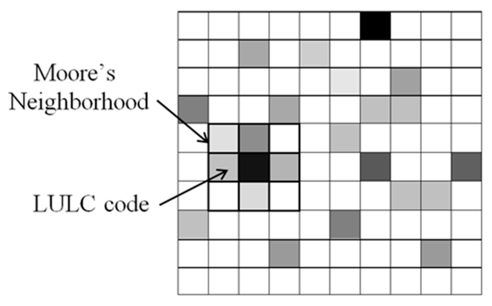
According to the definition of the CA model, it has five components: cell space, cell states, time steps, transition rules, and neighborhood. In this research, each map pixel was treated as one cell and the conventional 3 × 3 Moore’s neighborhood was adopted to identify and calculate the ‘spatial force’ from its neighbors (Figure 2). The LULC class was used as the cell state and the states of the neighboring cells were considered in determining the state of the center cell.
The transition rule determines the new state of each cell from the current state of the cell and the states of the cells in its neighborhood. The transition rule of CA in the LULC case of this study states that the current cell may change its state if there are state differences between the cell and its neighbors. For example, if the average membership of its neighboring cells for one LULC type is larger than the membership of the center cell, there will be a driving force from the neighbors to the center cell for this LULC type. The center cell’s state will be updated to the class having the highest transition probability among its neighbors. Let Dij represent the difference of membership between the center pixel and neighbor cells for LULC type i and j, and the minimum and maximum differences for each pair of class are and . The transition probability P(i, j) from the LULC type i to the LULC type j in each cell can be calculated by:
In this research, the transition rule was applied to derive the transition probability of cells, and the entire LULC grids were updated annually. As the real engines of change in CA, the transition rule specifies the cell’s behavior between time-step evolutions to determine the cell’s future state. Beside the transition probability derived from the historical LULC change using the MC model, the other transition suitability maps derived from elevation, slope, distance to road, and the socioeconomic drivers were integrated into the Markov-CA model to predict the future LULC change.
3.3. Integrating Markov-CA and Other Drivers
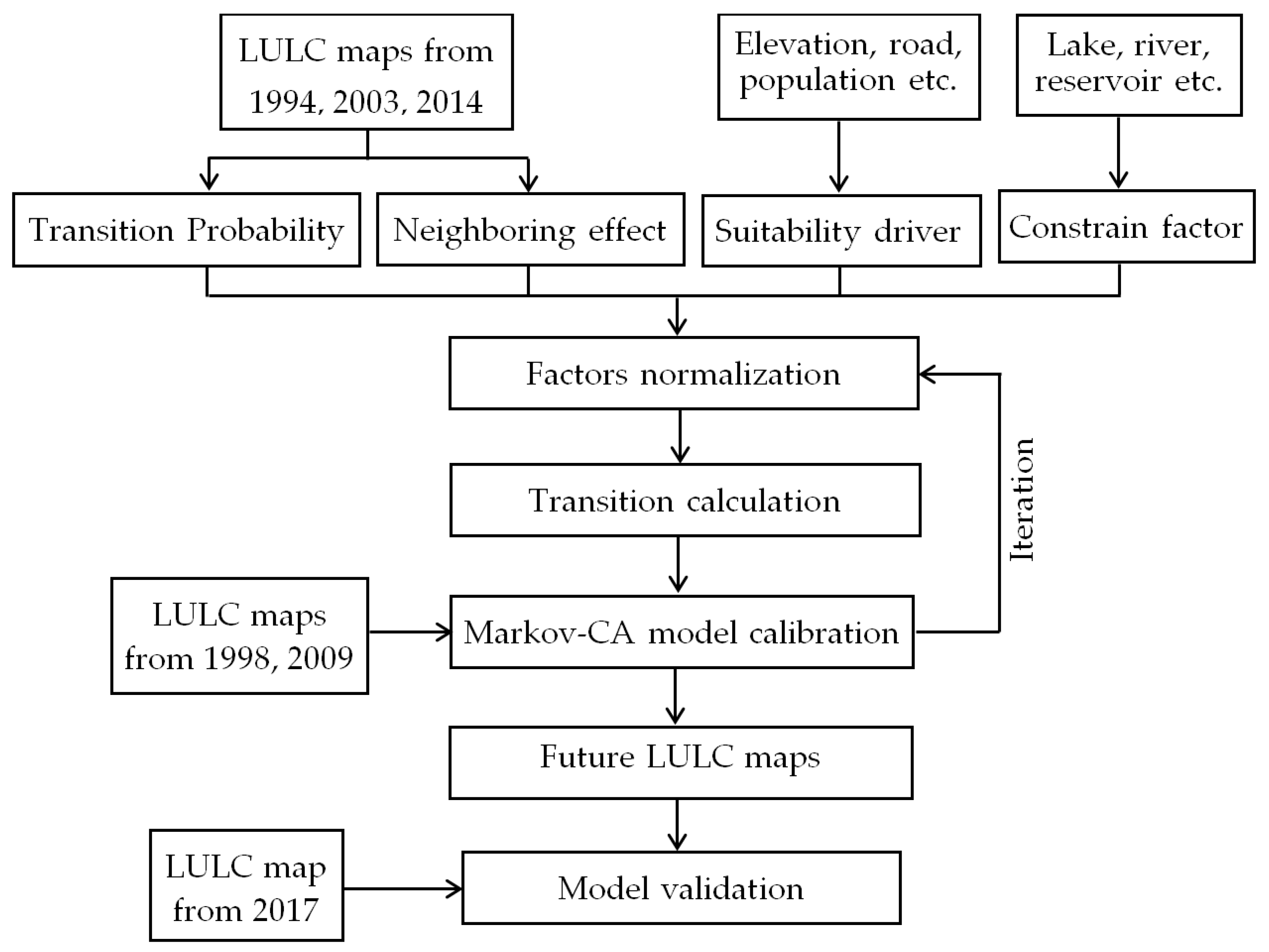
A systematic framework for the Markov-CA model is illustrated in Figure 3. The Markov-CA model was controlled by four driving forces: transition probability fp, neighboring effect fn, suitability driver fs, and constrain factor fc. The transition probability fp was derived from the historical transition MC model using Equation (3) and the neighboring effect fn was derived from the current cell status (Figure 2, Equation (4)). The constrain factor fc was based on the constrain layer, including the water, elevation, and slope (Figure 2), while the suitability driver fs represents the driving forces such as population and road density (Figure 2).
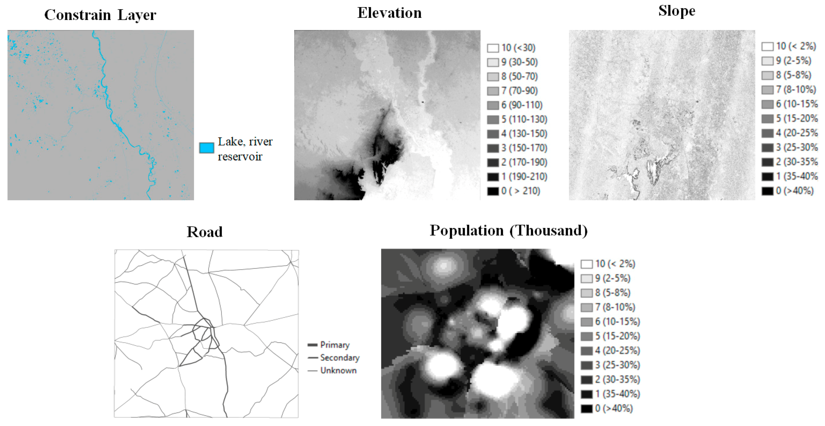
All driving forces were normalized into a fuzzy membership ranging from 0 to 1, which controlled the state of cells at time t + 1 according to the function . LULC change is a complex dynamics process that involves a number of environmental, social, and economic drivers [49]. The other factors that impact LULC change were defined and included in the transition rules as suitability drivers (e.g., elevation, distance to road, road density, and population growth) and constrain factors (e.g., lake, river, and reservoir) (Figure 4). For the census data, the city or town with a population of more than 10,000 were collected for the years 1991, 2001, and 2011, and population maps were generated using the Kriging function in Geostatistical Analysis of ArcGIS. The impact of each sustainability driver from neighbor cells was defined by the membership difference between the center cell and its neighbors as:
where SDxy is the normalized membership difference at location (x,y), is the membership difference in suitability drivers between the center cell and its neighbors, and n is the total number of neighbor cells.
3.4. Model Calibration and Validation
A critical step in the Markov-CA model is the calibration of the model to assign appropriate parameters for each input variable. In this research, two LULC maps classified from Landsat images acquired in 1998 and 2009 were used as empirical data. Each combination of four variables () denotes one solution and the weights are integers ranging from 0 to 100. Once the initial data and model code were chosen by the Monte Carlo random selection, the model was run at yearly intervals to represent one solution combination till the calibration years. The calibration data were the classified maps from the years 1998 and 2009. The parameter with the highest match was ranked and selected for the next year’s simulation. The detailed operation of this calibration method can be found in the papers by Shan et al. [71] and Al-Ahmadi et al. [72]. This step was repeated until the years of two calibration maps and the best parameters with the lowest discrepancy were selected as the model parameter.
The validation of the Markov-CA model was performed by comparing the predicted LULC map with the empirical map of the same year. The predicted LULC map was then overlaid with the empirical map of the year 2017 to visualize the spatial distribution of errors and to develop the error matrix for each class. The root-mean-square-error (RMSE) was used to evaluate the accuracy of the model as:
where Pe is the percentage of each class from the classified map, Pp is the percentage of each class from the empirical map, and N is the total number of LULC classes.
In order to evaluate the spatial distribution of the model performance, the empirical map and predicted results were overlaid to derive the accuracy matrix and then the user’s and producer’s accuracy of each class were calculated using this pixel-based accuracy matrix.
4. Results and Discussion
4.1. MC Transition Matrices from the Historical LULC Changes
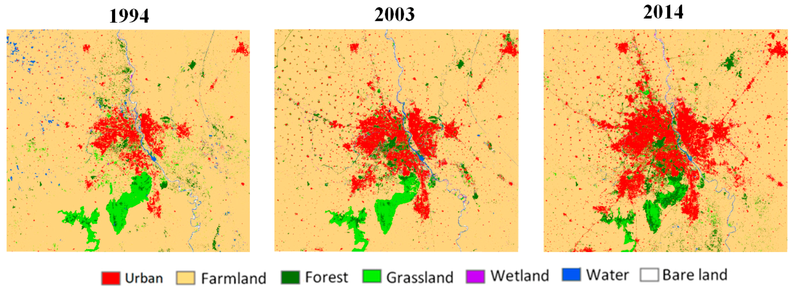
The LULC maps classified from 1994, 2003, and 2014 Landsat images are shown in Figure 5. The dominant LULC type is farmland, covering 7925.86 km2 and 78.98% of the study area in 2014. The urban area has a very similar size to grassland during the 1990s, but increased dramatically from 461.35 km2 (4.60%) in 1994 to 1273.55 km2 (12.69%) in 2014. The obvious urban sprawl was found in the North West and South West Districts in Delhi due to the rapid population growth and immigration, as well as the area along the major transportation routes. These initial change analyses help us to identify roads and the population as two suitability drivers in the model development.
The total change areas between 1994 and 2003 and between 2003 and 2014 were 1190.81 km2 and 1311.58 km2 and the percentage change were 11.87% and 13.07%, respectively. The dominant LULC class, farmland, decreased from 8745.56 km2 in 1994 to 8389.11 km2 in 2003 and to 7949.97 km2 in 2014. The most significant changes were farmland loss to urban, which were 43.54% and 50.64%, respectively, of the total area of farmland loss. This result indicates that significant farmland has been lost in the study area during the last two decades due to its rapid urbanization.
The MC transition matrices were calculated based on the classified maps to determine the landscape change (Table 3 and Table 4). Within the transition table, each value represents the total changed area and percentage from the starting year (column side) to the ending year (row side). The annual transition probability matrix was further derived using Equations (2) and (3), by accumulating from these two periods (Table 5). By examining the detailed landscape change data (Table 3, Table 4 and Table 5), it is clear that the change from farmland to urban was the largest change, followed by the change from farmland to natural vegetation (forest and grassland). This result indicates an obvious farmland loss during the last two decades in the study area. The yearly transition probability was incorporated into the Markov-CA model for the annual updates in the model prediction.
4.2. Predicted LULC Change Using Markov-CA Model
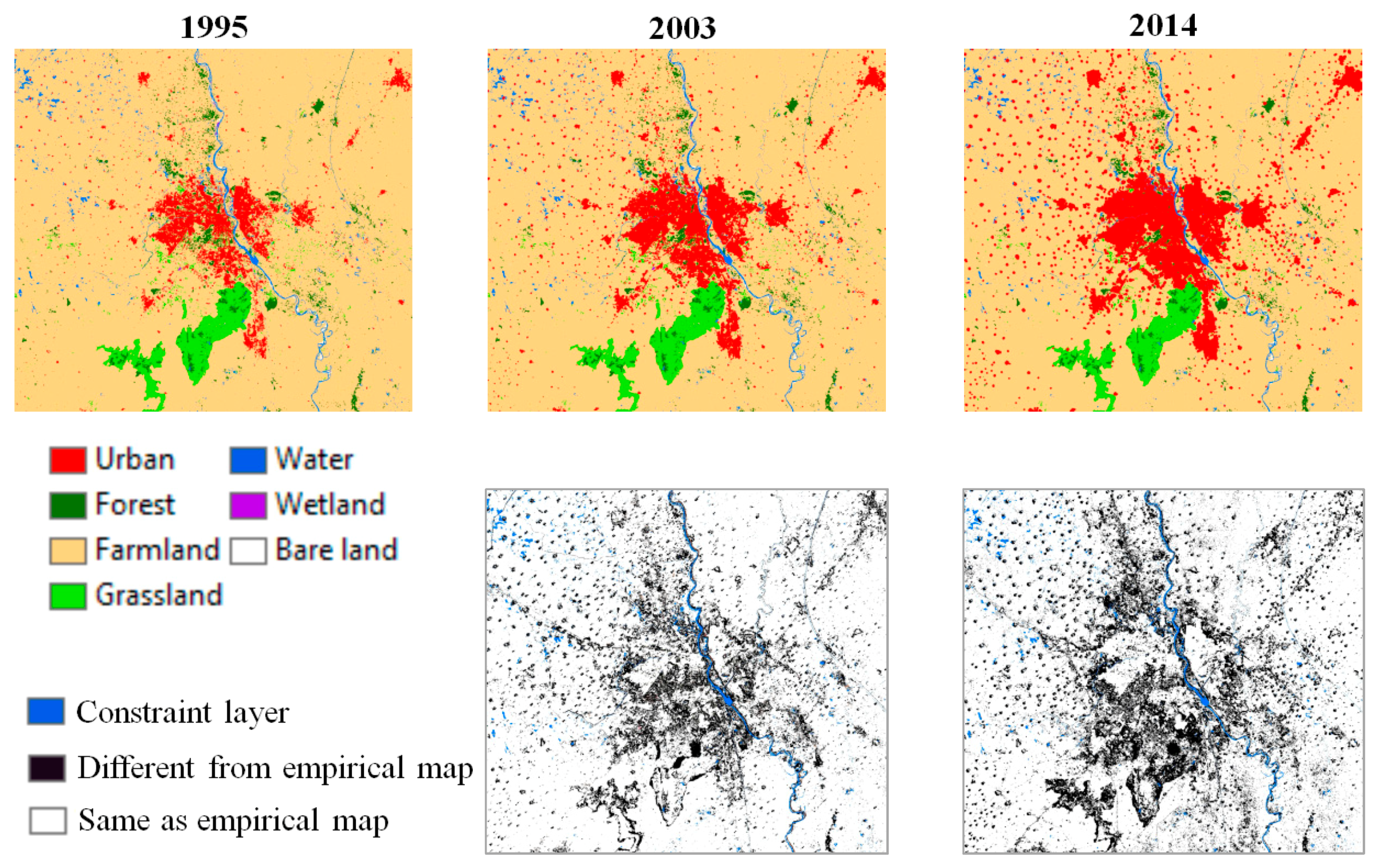
Our algorithm (Figure 3) was scripted and implemented in the Matlab and IDL/ENVI using the landscape maps for 1994, 2003, and 2014. The first set of annual maps was produced using only the Markov-CA model, without considering other driving factors. In order to illustrate the changing pattern and model simulation results, the three simulated maps in the years 1995, 2003, and 2014 are listed in Figure 6. The simulated LULC maps in 2003 and 2014 were further overlaid with the actual classified map to display the simulation quality of the Markov-VA model. Obviously, the predicted result in 2003 is better than the result in 2014, particular in the forest and grassland in the suburban area, with less difference compared to the empirical maps (Figure 6). This might be caused by the error propagation as the predicted result from the current year will be the input data for the next year’s simulation. The error was accumulated not only from the model itself, but also the initial image classification. For example, the low accuracy in grassland led to the low accuracy of grassland in our model prediction (Table 2 and Figure 6). The landscape types with a less direct connection to the socioeconomic drivers, e.g., grassland, wetland, bare land, and water, have a lower accuracy than the socioeconomic-related landscapes. Meanwhile, the accumulated error increased over time and offset the advantage of our model.
As indicated in the figures, the urban area will continue to grow in the same pattern since the expansion area will be located next or close to the existing urban areas. During the last two decades, the dominant LULC class was farmland, as it covers more than 70% of the study area. In our results, the initial predicted results showed that the increasing urban area from 1995 to 2005 was 401 km2, which was less than the increased urban area (455 km2) from 2005 to 2015. This might have been caused by the rapid urbanization in New Delhi after the 2000s. Urbanization and its subsequent landscape change are usually driven by many other factors, such as population growth, economic development, and government policies. Incorporating more drivers will help to develop better prediction results.
In our simulated landscape maps, the best predictable type of urban growth is the outward expansion of urban area in the suburban area in the Markov-CA model [73]. As the “spreading” runs in a repeated model in CA, the “changing” area in the suburban area can be easily predicted. In this study, the predicted area can be easily turned into a homogeneous and isolated “island”; however, it is hard or even impossible to predict the “emergent” centers, which might be caused by the local policy or even population growth/migration.
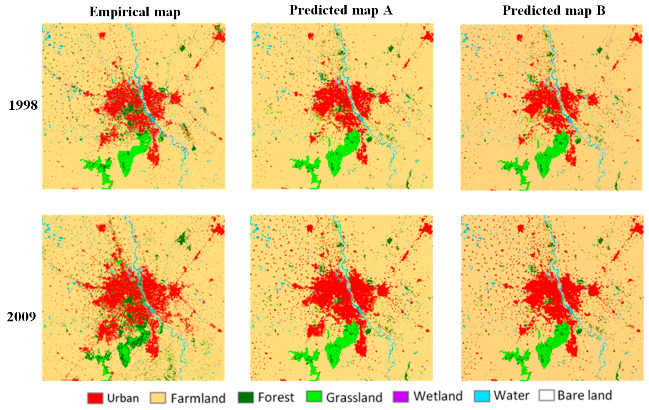
Different from the previous widely used Markov-CA model, our model further incorporated other socioeconomic drivers into the model (Figure 3). The advantage of our model is that it can incorporate various socioeconomic developments, which might be major drivers of urban sprawls in our study area. To measure the improvement as a result of the incorporation of these drivers, the predicted results from our model (namely full Markov-CA model) and the Markov-CA model without drivers (namely “only” Markov-CA model) were compared with the empirical maps that were derived by classifying the Landsat images (in 1998 and 2009) (Figure 7). The maps B are the predicted results derived by “only” the Markov-CA model, while the maps A are the results from our model. In the predicted map in the year of 1998, the urban area was 744 km2 and 747 km2 in the “only” Markov-CA model and our model, respectively while the empirical map was 774 km2. In 2009, our predicted urban area was 1163 km2 and the “only” Markov-CA model was 1144 km2 while the area in the empirical map was 1196 km2. This comparison indicated that the improvements in the map derived by our model for 1998 are not as obvious as the improvements in the map derived by our model for 2009, especially for the “new” urban centers far away from the existing urban area. These differences could be found in the South West and North West districts, the most rapid developing districts in Delhi. The population growth in these two districts was rapid, contributing 41.98% of the total population growth in Delhi [63]. The large area of farmland in these two districts provides the potential “developable” area for urban expansion. Rapid urbanization in these two districts led to the development of various new settlements, including the informal Jhuggis and Jhoparis resettlement colonies, refugee resettlement colonies, slum resettlement colonies, authorized/planned colonies, unauthorized-regularized colonies, urbanized village/colonies, etc. [59]. The incorporated drivers, especially the population change, help our model to predict these changes.
A detailed comparison of the empirical maps and the simulated results from two models were conducted and the results are shown in Table 6. Obviously, our model coincided more with the empirical map, especially in the predicted farmland and urban area. Although the RMSE increased from the year 1998 to 2009 due to the error propagation, our model improved the simulation result by incorporating other driving factors. Although the “full” model can predict better than the “only” model, the improvement in the “full” model is not very evident, especially for the early prediction. For example, the RMSE only decreased from 0.61 (“only” model) to 0.60 (“full” model) in 1998, while the decrease in RMSE is more noticeable in 2009 (from 1.96 to 1.89). The possible reason for this is that the length of prediction time is a significant factor that determines the RMSE. The longer the prediction time, the larger RMSE will be. Meanwhile, the socioeconomic development is not that substantial in a short period of time, which will limit the function of socioeconomic factors.
In the further analysis between the “only” model and “full” model in Table 6, it could be noted that the socioeconomic drivers influenced different LULC types differently. The most obvious improvement could be found in urban and farmland, which were more related to the socioeconomic drivers. Obviously, the heterogeneous pattern of socioeconomic factors in urban or farmland was more evident than the nature-related LULC classes and this helped the “full” model to predict. While other LULC classes were not highly related to socioeconomic development, the improvements were not very obvious. Another advantage of our model is for long-term prediction, since the socioeconomic development usually needs decades. The input of socioeconomic drivers could help the model simulation in the “correct” track.
4.3. Model Validation
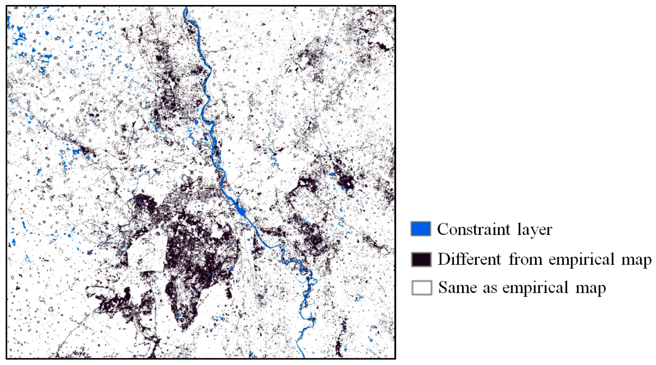
In order to validate our model, the simulated map was overlaid with the empirical map for the same year. Two stages were used in the validation: visual inspection and quantitative evaluation. Figure 8 shows the agreement and disagreement components between the simulated map and the corresponding empirical map in 2017. Obviously, the most accurate predicted classes were urban and farmland. Although there are many errors found along the boundary of the small towns, the majority of the large city area, especially the most populated area, has a relatively higher accuracy than other classes. With socioeconomic variables being considered, this model is more applicable to the human-disturbed landscapes, such as urban area and farmland.
In order to further validate the model prediction, a confusion matrix among land use types between the empirical map and predicted map was developed (Table 7). The table shows the comparisons and agreements between the simulated result and empirical map, and both user’s accuracy and producer’s accuracy were calculated and listed in Table 7. In this research, the best predicted class is farmland (with 89.08 user’s accuracy and 95.07% producer’s accuracy), followed by the urban area (user’s accuracy 82.60% and producer’s accuracy 74.04%). The natural LULC classes, particularly the classes with small areas, have a relatively low accuracy. The possible reason for this poor performance is the frequent seasonal/annual fluctuations among these natural classes. The largest error was found between forest and grassland (126 km2), followed by the error between grassland and farmland (105 km2). These two errors caused the low accuracy in both grassland and forest. Yamuna River, the longest and the second largest tributary river of the Ganges River in northern India, is the major river in the study area and its major water source is the Yamunotri Glacier. During the last two decades, Yumuna River has experienced a decrease in water quality due to population growth and irrigation use, as well as a fluctuation in water discharge due to the seasonal melting of the glacier [74]. These unexpected changes in water area, as well as the nearby wetland and bare land, are hard to predict and the simulation for the natural landscapes needs more input drivers or information.
4.4. Future Farmland Trajectories
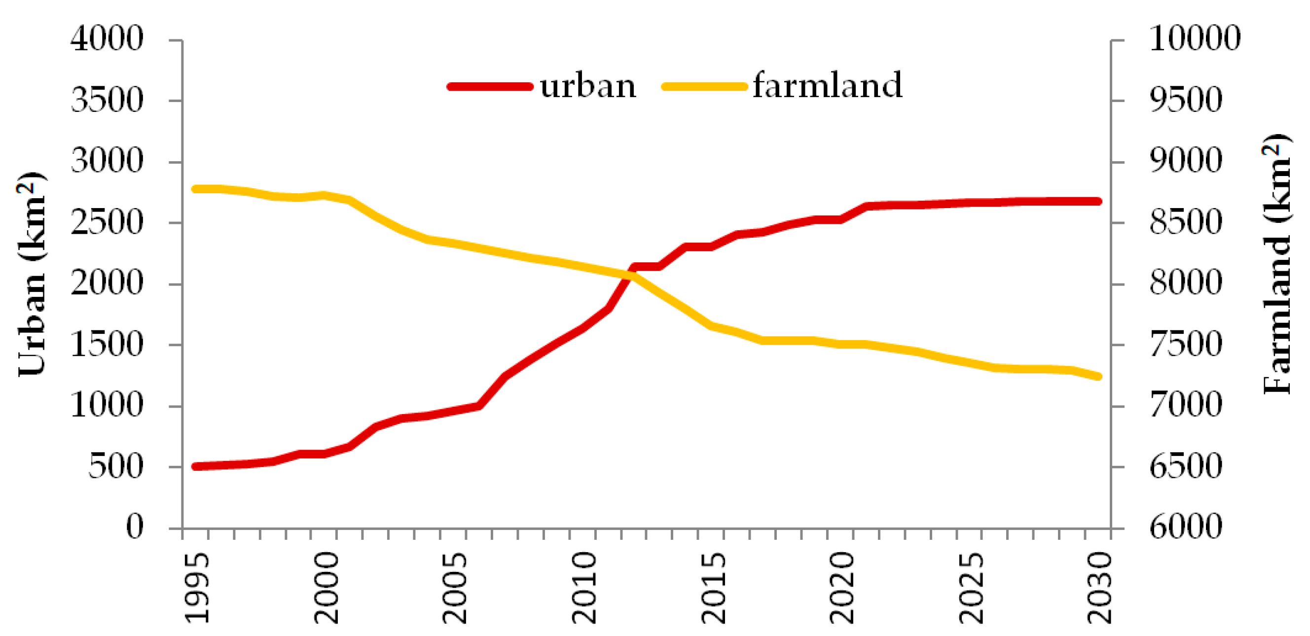
As the national capital city of India, Delhi has experienced rapid LULC change as the result of population growth and numerous migrants. Our model was used to predict the LULC change from 1995 to 2030 at yearly steps. From each predicted map, the area of two dominant LULC classes, farmland and urban area, was calculated to analyze the past and future trajectories of farmland loss due to rapid urbanization. In the simulated result, the farmland has a consistent decreasing trend from the 1990s and the trend continues to 2030, while the urban area, on the other hand, keeps on increasing from 1995 to 2030. Specifically, the urban area will increase from 504.13 km2 to 2679.54 km2 and farmland will decrease from 8778.19 km2 to 7242.94 km2. Over the last two decades and next fifteen years, rapid urbanization was and will still be the dominant change in the study area, which is the major reason for the farmland loss.
Although the change patterns of urban and farmland are in the opposite directions, their change rates are different. The farmland has a relatively stable decreasing pattern from 1995 to 2030, while the increase rates of change of urban areas are larger during 2000s to 2020 than during the other periods (Figure 9). This predicted result is consistent with the intensive urbanization in Delhi from the 2000s. The rapid urbanization leads to the development of urban forms with the destruction of other land use, particularly farmland from the 2000s [75]. Based on the predicted result, this rapid urbanization in Delhi will continue until 2020 and slow down from 2020 to 2030.
Besides the significant change from farmland to urban, the change from farmland to forest/grassland was also obvious. The change from farmland to forest/grassland was caused by the forest recovery policy [76], e.g., the native forest cover decreased before 2000 and then increased due to reforestation policy. Therefore, this recovery is the major reason for the farmland loss to forest. Another reason for the farmland loss is the misclassification, especially between farmland and grassland. Although the selected images are both in growing seasons (e.g., September in 1994 and March in 2003), a spectral difference between September and March exists, which caused the misclassification among cropland and grassland and led to the error in model prediction. A further phenology analysis between cropland and forest/grassland is needed to improve classification in the future.
5. Conclusions
Modeling LULC change under rapid urbanization is crucial for environmental management and enables us to better understand the future LULC change. The spatial-temporal prediction of LULC using multitemporal Landsat imagery and the Markov-CA model helps us to identify the past and future trajectories of farmland loss in Delhi from 1990s due to rapid urbanization. This study explored the potential of other socioeconomic drivers, particularly population growth, to improve the Markov-CA model and the improved model has been proved as a practical and effective one to simulate and predict the LULC change in rapid urbanization areas.
The Markov-CA model has indicated the farmland loss in the study area from historical 1990s to the future in 2030. The spatial-temporal model provides not only a quantitative description of change in the past, but also the direction and magnitude of change in the future. However, there are several limitations that can be improved in future studies:
- The accuracy assessment of the model was performed directly by overlaying the predicted result with the classified map. However, the error of the model was accumulated from the data source, data processing, and prediction models. How to develop a more robust method to assess these errors is an interesting topic to be explored;
- The development of the study area was highly related to the rapid urbanization, particularly, population growth and economic development. However, it does not incorporate other important driving factors, such as climate, policy, and other human disturbance. Incorporating more critical factors will improve our model prediction in te future work;
- Although multiple socioeconomic drivers were considered in our model, we treated each variable equally by calculating the different membership between the center cell and its neighbor cells at the same time (Equation (5)). Treating these variables differently and assigning different weights to different socioeconomic factors will improve our model accuracy in the future;
- The model incorporated the driving factors through the neighborhood effect and Markov transition probability linearly. This linear combination may be not true in reality and needs more study to improve it. Finding dynamic and appropriate model parameters will improve this model and is recommended for future study.
Author Contributions
Both the author and coauthor have made significant contributions to the conception, design, and interpretation of the reported study. This study was part of a funded research project, of which L.D. is the principal investigator. Identified research question and objectives: J.T. and L.D.; collected and processed the remote sensing data: J.T.; designed the methodology: J.T.; interpreted the research results and validation: J.T., L.D.; writing—original draft preparation: J.T.; writing—reviewing, editing, and finalizing the manuscript: L.D.
Funding
This study is supported by the National Aeronautic and Space Administration (NASA) through the Land Use and Land Cover program (Award # NNX17AH95G).
Acknowledgments
The authors would like to take this opportunity to thank members of the editorial board and anonymous reviewers for their useful and constructive comments.
Conflicts of Interest
The authors declare no conflict of interest.
References
- Mohan, M.; Pathan, S.K.; Narendrareddy, K.; Kandya, A.; Pandey, S. Dynamics of urbanization and its impact on land-use/land-cover: A case study of megacity Delhi. J. Environ. Prot. 2011, 2, 1274–1283. [Google Scholar] [CrossRef]
- Tang, J.; Di, L.; Xiao, J.; Lu, D.; Zhou, Y. Impacts of land use and socioeconomic patterns on urban heat island. Int. J. Remote Sens. 2017, 38, 3445–3465. [Google Scholar] [CrossRef]
- United Nations. World’s Population Increasingly Urban with More Than Half Living in Urban Areas. Available online: http://www.un.org/en/development/desa/news/population/world-urbanization-prospects-2014.html (accessed on 7 March 2018).
- Kalnay, E.; Cai, M. Impact of urbanization and land-use change on climate. Nature 2003, 423, 528–531. [Google Scholar] [CrossRef] [PubMed]
- Grimm, N.B.; Faeth, S.H.; Golubiewski, N.E.; Redman, C.L.; Wu, J.; Bai, X.; Briggs, J.M. Global change and the ecology of cities. Science 2008, 319, 756–760. [Google Scholar] [CrossRef] [PubMed]
- Tang, J.; Wang, L.; Yao, Z. Analyses of urban landscape dynamics using multi-temporal satellite images: A comparison of two petroleum-oriented cities. Landsc. Urban Plan. 2008, 87, 269–278. [Google Scholar] [CrossRef]
- Deng, J.S.; Wang, K.; Hong, Y.; Qi, J.G. Spatio-temporal dyanmics and evolution of land use change and landscape pattern in response to rapid urbanization. Landsc. Urban Plan. 2009, 92, 187–198. [Google Scholar] [CrossRef]
- Jiang, L.; O’Neill, B.C. Global urbanization projections for the shared socioeconomic pathways. Glob. Environ. Chang. 2017, 42, 193–199. [Google Scholar] [CrossRef]
- Bounoua, L.; Safia, A.; Masek, J.; Peter-Lidard, C. Impact of urban growth on surface climate: A case study in Organ, Algeria. J. Appl. Meteorol. Clim. 2008, 48, 217–232. [Google Scholar] [CrossRef]
- Pandey, B.; Seto, K.C. Urbanization and agricultural land loss in India: Comparing satellite estimates with census data. J. Environ. Manag. 2015, 148, 53–66. [Google Scholar] [CrossRef]
- Jiang, L.; Deng, X.; Seto, K.C. The impact of urban expansion on agricultural land use intensity in China. Land Use Policy 2013, 35, 33–39. [Google Scholar] [CrossRef]
- Reddy, V.R.; Reddy, B.S. Land alienation and local communities: Case studies in Hyderabad-Secunderabad. Econ. Political Wkly. 2007, 42, 3233–3240. [Google Scholar]
- Varughese, G.; Lakshmi, K.; Kumar, A.; Rana, N. State of Envioenment Report: India, 2009; India Environment Portal: New Delhi, India, 2009; pp. 123–136. [Google Scholar]
- Veni, L.K.; Alivelu, G. Production and per capita availability of food grains in India-an analysis. IUP J. Agric. Econ. 2005, 2, 18–33. [Google Scholar]
- Brahmanand, P.S.; Kumar, A.; Ghosh, S.; Roy Chowdhury, S.; Singandhupe, R.B.; Singh, R.; Nanda, P.; Chakraborthy, H.; Srivastava, S.K.; Behera, M.S. Challenges of food security in India. Curr. Sci. 2013, 104, 841–846. [Google Scholar]
- Kalamkar, S.S. Urbanisation and agricultural growth in India. Indian J. Agric. Econ. 2009, 64, 442–461. [Google Scholar]
- Tang, J.; Chen, F.; Schwartz, S.S. Assessing spatiotemporal variations of greenness in the Baltimore-Washington corridor area. Landsc. Urban Plan. 2012, 105, 296–306. [Google Scholar] [CrossRef]
- Sharma, R.; Joshi, P.K. Mapping environmental impacts of rapid urbanization in the national capital region of India using remote sensing inputs. Urban Clim. 2016, 15, 70–82. [Google Scholar] [CrossRef]
- Gomarasca, M.; Brivio, P.; Pagnoni, F.; Galli, A. One century of land use change in the metropolitan area of Milan (Italy). Int. J. Remote Sens. 1993, 14, 211–223. [Google Scholar] [CrossRef]
- Lenney, M.; Woodcock, C.; Collins, J.; Hamdi, H. The status of agricultural lands in Egypt: The use of multitemporal NDVI features derived from landsat TM. Remote Sens. Environ. 1996, 56, 8–20. [Google Scholar] [CrossRef]
- Farooq, S.; Ahmad, S. Urban sprawl development around Aligarh city: A study aided by satellite remote sensing and GIS. J. Indian Soc. Remote Sens. 2008, 36, 77–88. [Google Scholar] [CrossRef]
- Sandhya Kiran, G.; Joshi, U.B. Estimation of variable explaining urbanization concomitant with land-use change: A spatial approach. Int. J. Remote Sens. 2013, 34, 824–847. [Google Scholar] [CrossRef]
- Wakode, H.B.; Baier, K.; Jha, R.; Azzam, R. Analysis of urban growth using landsat TM/ETM data and GIS-a case study of Hyderabad, India. Arab. J. Geosci. 2013, 16, 1–13. [Google Scholar] [CrossRef]
- Tang, J. Modeling urban landscape dynamics using subpixel fractions and fuzzy cellular automata. Environ. Plan. B 2011, 38, 903–920. [Google Scholar] [CrossRef]
- Mertens, B.; Lambin, E.F. Land cover change trajectories in Southern Cameroon. Ann. Assoc. Am. Geogr. 2000, 90, 467–494. [Google Scholar] [CrossRef]
- Tang, J.; Wang, L.; Yao, Z. Spatio-temporal urban landscape change analysis using the Markov chain model and a modified genetic algorithm. Int. J. Remote Sens. 2007, 28, 3255–3271. [Google Scholar] [CrossRef]
- Liu, M.; Hu, Y.; Chang, Y.; He, Y.; Zhang, W. Land use and land cover change analysis and prediction in the upper reaches of the Minjiang River, China. Environ. Manag. 2009, 43, 899–907. [Google Scholar] [CrossRef] [PubMed]
- Joshi, N.; Baumann, M.; Ehammer, A.; Fensholt, R.; Grogan, K.; Hostert, P.; Jepsen, M.; Kuemmerle, T.; Meyfroidt, P.; Mitchard, E.; et al. A review of application of optical and radar remote sensing data fusion to land use mapping and monitoring. Remote Sens. 2016, 8, 70. [Google Scholar] [CrossRef]
- Alqurashi, A.F.; Kumar, L.; Sinha, P. Urban land cover change modeling using time-series satellite images: A case study of urban growth in five cities of Saudi Arabia. Remote Sens. 2016, 8, 838. [Google Scholar] [CrossRef]
- Cromley, R.G.; Hanink, D.M. Coupling land-use allocation models with raster GIS. J. Geogr. Syst. 1999, 1, 137–153. [Google Scholar] [CrossRef]
- Herold, M.; Goldstein, N.C.; Clarke, K.C. The spatiotemporal form of urban growth: Measurement, analysis and modeling. Remote Sens. Environ. 2003, 86, 286–302. [Google Scholar] [CrossRef]
- Eastman, R. Guide to GIS and Image Processing; Clark University: Worcester, MA, USA, 1999; pp. 110–125. [Google Scholar]
- Tobler, W.R. Cellular Geography. In Philosophy in Geography; Gale, S., Olsson, G., Eds.; D. Reidel Publishing Company: Dordrecht, The Netherlands, 1979; pp. 179–186. [Google Scholar]
- Veldkamp, A.; Fresco, L.O. CLUE: A conceptual model to study the conversion of land use and its effects. Ecol. Model. 1996, 85, 253–270. [Google Scholar] [CrossRef]
- Adhikari, S.; Southworth, J. Simulating forest cover changes of Bannerghatta National Park based on a CA-Markov model: A remote sensing approach. Remote Sens. 2012, 4, 3215–3243. [Google Scholar] [CrossRef]
- Hegazy, I.R.; Kaloop, M.R. Monitoring urban growth and land use change detection with GIS and remote sensing techniques in Daqahia governorate Egypt. Int. J. Sustain. Built Environ. 2015, 4, 117–124. [Google Scholar] [CrossRef]
- Zheng, H.W.; Shen, G.Q.; Wang, H.; Hong, J. Simulating land use change in urban renewal areas: A case study in Hong Kong. Habitat Int. 2015, 46, 23–34. [Google Scholar] [CrossRef]
- Weng, Q. Land use change analysis in the Zhujiang delta of China using satellite remote sensing, GIS and stochastic modeling. J. Environ. Manag. 2002, 64, 273–284. [Google Scholar] [CrossRef]
- Parker, C.D.; Manson, M.S.; Janssen, A.M.; Hoffmann, J.M.; Deadman, P. Multi-agent systems for the simulation of land-use and land-cover change: A review. Ann. Assoc. Am. Geogr. 2003, 93, 314–337. [Google Scholar] [CrossRef]
- Halmy, M.W.; Gessler, P.E.; Hicke, J.A.; Salem, B.B. Land use/land cover change detection and prediction in the north-western coastal desert of Egypt using Markov-CA. Appl. Geogr. 2015, 63, 101–112. [Google Scholar] [CrossRef]
- Bourne, L.S. Monitoring change and evaluating the impact of planning policy on urban structure: A Markov chain experiment. Plan. Can. 1976, 16, 5–14. [Google Scholar]
- Muller, M.R.; Middleton, J.A. Markov model of land-use change dynamics in the Niagara Region, Ontario, Canada. Landsc. Ecol. 1994, 9, 151–157. [Google Scholar]
- Moghadam, H.S.; Helbich, M. Spatiotemporal urbanization processes in the megacity of Mumbai, India: A Markov chains-cellular automata urban growth model. Appl. Geogr. 2013, 40, 140–149. [Google Scholar] [CrossRef]
- Yang, X.; Zheng, X.; Chen, R. A land use change mode: Integrating landscape pattern indexes and Markov-CA. Ecol. Model. 2014, 283, 1–7. [Google Scholar] [CrossRef]
- Batty, M.; Xie, Y. From cells to cities. Environ. Plan. B 1994, 21, 31–48. [Google Scholar] [CrossRef]
- Aburas, M.M.; Ho, Y.M.; Ramli, M.F.; Ash’aari, Z.H. Improving the capability of an integrated CA-Markov model to simulate spatio-temporal urban growth trends using an analytical hierarchy process and frequency ratio. Int. J. Appl. Earth Obs. 2017, 59, 65–78. [Google Scholar] [CrossRef]
- Clarke, K.C.; Hoppen, S. A self-modifying cellular automata model of historical urbanization in the San Francisco Bay area. Environ. Plan. B 1997, 24, 247–261. [Google Scholar] [CrossRef]
- Wu, F.; Martin, D. Urban expansion simulation of Southeast England using population surface modeling and cellular automata. Environ. Plan. A 2002, 34, 1855–1876. [Google Scholar] [CrossRef]
- Mas, J.; Kolb, M.; Paegelow, M.; Olmedo, M.; Houet, T. Inductive pattern-based land use/cover change models: A comparison of four software packages. Environ. Model. Softw. 2014, 51, 94–111. [Google Scholar] [CrossRef] [Green Version]
- Kamusoko, C.; Aniya, M.; Adi, B.; Manjoro, M. Rural sustainability under threat in Zimbabwe-Simulation of future land use/cover changes in the Bindura district based on the Markov-cellular automata model. Appl. Geogr. 2009, 29, 435–447. [Google Scholar] [CrossRef]
- Ghosh, P.; Mukhopadhyay, A.; Chanda, A.; Mondal, P.; Akhand, A.; Mukherjee, S.; Nayak, S.K.; Ghosh, S.; Mitra, D.; Ghosh, T.; et al. Application of cellular automata and Markov-chain model in geospatial environmental modeling—A review. Remote Sens. Appl. 2017, 5, 64–77. [Google Scholar] [CrossRef]
- Pontius, G.R.; Malanson, J. Comparison of the structure and accuracy of two land change models. Int. J. Geogr. Inf. Syst. 2005, 19, 243–265. [Google Scholar] [CrossRef]
- Eastman, J.R. IDRISI Guide to GIS and Image Processing; Clark University: Worcester, MA, USA, 2009; pp. 182–185. [Google Scholar]
- Theobald, D.M.; Hobbs, N.T. Forecasting rural land-use change: A comparison of regression- and spatial transition-based models. Geogr. Environ. Model. 1998, 2, 65–82. [Google Scholar]
- Tolessa, T.; Senbeta, F.; Kidane, M. The impact of land use/land cover change on ecosystem services in the central highlands of Ethiopia. Ecosyst. Serv. 2017, 23, 47–54. [Google Scholar] [CrossRef]
- Liyama, N.; Kamada, M.; Nakagoshi, N. Ecological and social evaluation of landscape in a rural area with terraced paddies in southwestern Japan. Landsc. Urban Plan. 2005, 73, 60–71. [Google Scholar]
- Lee, C.; Huang, S.; Chan, S. Biophysical and system approaches for simulating land-use change. Landsc. Urban Plan. 2008, 86, 187–203. [Google Scholar] [CrossRef]
- Jain, M.; Dawa, D.; Mehta, R.; Dimri, A.P.; Pandit, M.K. Monitoring land use change and its drivers in Delhi, India using multi-temporal satellite data. Model. Earth Syst. Environ. 2016, 2, 1–14. [Google Scholar]
- Rahman, A.; Kumar, S.; Fazal, S.; Siddiqui, M.A. Assessment of land use/land cover change in the north-west district of Delhi using remote sensing and GIS techniques. J. Indian Soc. Remote Sens. 2012, 40, 689–697. [Google Scholar] [CrossRef]
- Vogelmann, J.E.; Helder, D.; Morfit, R.; Choate, M.J.; Merchant, J.W.; Bulley, H. Effects of Landsat 5 Thematic Mapper and Landsat 7 Enhanced Thematic Mapper Plus radiometric and geometric calibrations and corrections on landscape characterization. Remote Sens. Environ. 2001, 78, 55–70. [Google Scholar] [CrossRef] [Green Version]
- Fu, P.; Weng, Q. A time series analysis of urbanization induced land use and land cover change and its impact on land surface temperature with Landsat imagery. Remote Sens. Environ. 2016, 175, 205–214. [Google Scholar] [CrossRef]
- Datta, K.K.; Jong, C.D. Adverse effect of waterlogging and soil salinity on crop and land productivity in northwest region of Haryana, India. Agric. Water Manag. 2002, 57, 223–238. [Google Scholar] [CrossRef]
- Census of India. Available online: http://www.censusindia.gov.in/ (accessed on 20 May 2018).
- Alexander, P.; Rounsevell, M.D.A.; Dslich, C.; Dodson, J.R.; Engstrom, K.; Moran, D. Drivers of global agricultural land use change: The nexus of diet, population, yield, and bioenergy. Glob. Environ. Chang. 2015, 35, 138–147. [Google Scholar] [CrossRef]
- Fortin, M.J.; Boots, B.; Csillag, F.; Remmel, T.K. On the role of spatial stochastic models in understanding landscape indices in ecology. Oikos 2003, 102, 203–212. [Google Scholar] [CrossRef]
- Pattern, T.A.; Thomas, L.; Wilcox, C.; Ovaskainen, O.; Matthiopoulos, J. State-space models of individual animal movement. Trends Ecol. Evol. 2008, 23, 87–94. [Google Scholar] [CrossRef]
- Bichi, M.; Ripaccioli, G.; Cairano, S.D.; Bernardini, D.; Bemporad, A.; Kolmanovsky, I.V. Stochastic model predictive control with driver behavior leaning for improved powertrain control. In Proceedings of the 49th IEEE Conference on Decision and Control, Atlanta, GA, USA, 15–17 December 2010. [Google Scholar]
- Brown, D.G.; Pijanowski, B.C.; Duh, J.D. Modeling the relationships between land use and land cover on private lands in the Upper Midwest, USA. J. Environ. Manag. 2000, 59, 247–263. [Google Scholar] [CrossRef] [Green Version]
- White, R.; Engelen, G. Ceullular automata as the basis of integrated dynamics regional modeling. Environ. Plan. B 1997, 24, 235–246. [Google Scholar] [CrossRef]
- He, C.; Okada, N.; Zhang, Q.; Shi, P.; Li, J. Modeling dynamic urban expansion processes incorporating a potential model with cellular automata. Landsc. Urban Plan. 2008, 86, 79–91. [Google Scholar] [CrossRef]
- Shan, J.; Alkheder, S.; Wang, J. Genetic algorithm for the calibration of cellular automata urban growth modeling. Photogramm. Eng. Remote Sens. 2008, 74, 1267–1277. [Google Scholar] [CrossRef]
- Al-Ahmadi, K.; See, L.; Heppenstall, A.; Hogg, J. Calibration of a fuzzy cellular automata model or urban dynamics in Saudi Arabia. Ecol. Complex. 2009, 6, 80–101. [Google Scholar] [CrossRef]
- Clarke, K.C.; Gaydos, L.J. Loose-coupling a cellular automata model and GIS: Long-term urban growth prediction for San Francisco and Washington/Baltimore. Int. J. Geogr. Inf. Sci. 1998, 12, 699–714. [Google Scholar] [CrossRef] [PubMed]
- Misra, A.K. A river about to die: Yamuna. J. Water Res. Prot. 2010, 2, 489–500. [Google Scholar] [CrossRef]
- Ramachandra, T.V.; Bharath, A.H.; Sowmyashree, M.V. Monitoring urbanization and its implications in a mega city from space: Spatiotemporal patterns and its indicators. J. Environ. Manag. 2015, 148, 67–81. [Google Scholar] [CrossRef]
- Adhikari, S.; Southworth, J.; Nagendra, H. Understanding forest loss and recovery: A spatiotemporal analysis of land change in and around Bannerghatta National Park, India. J. Land Use Sci. 2014, 10, 402–424. [Google Scholar] [CrossRef]
Figure 1.
Study site—National Capital Region (NCR) of India.

Figure 2.
The cellular space and neighbors of simulated LULC change.

Figure 3.
Flowchart of the Markov-CA model.

Figure 4.
The example maps that were used to create the suitability drivers and constrain layers.

Figure 5.
The LULC maps from 1994 to 2014 used to derive the MC transition probability matrices.

Figure 6.
The simulated LULC maps and error maps.

Figure 7.
The comparison between the classified map and the predicted maps. Note: Predicted maps A were predicted with the incorporation of other drivers and predicted maps B were predicted with “only” the Markov-CA model.
Figure 7.
The comparison between the classified map and the predicted maps. Note: Predicted maps A were predicted with the incorporation of other drivers and predicted maps B were predicted with “only” the Markov-CA model.

Figure 8.
Map showing the spatial differences between the predicted map and the empirical map in 2017.
Figure 8.
Map showing the spatial differences between the predicted map and the empirical map in 2017.

Figure 9.
The predicted urban and farmland from 1995 to 2030.


Table 1.
Landsat images collected in this research.
| Path/Row | Acquisition Date (Year Month Day) | Sensor and Data Characteristics | Data Utility |
|---|---|---|---|
| 146/40 | 1994 09 30 | TM, 7 spectral bands, 30 m spatial resolution | Model development |
| 2003 03 07 | ETM, 8 spectral bands, 30 m spatial resolution | ||
| 2014 09 21 | OLI, 11 spectral bands, 15 m spatial resolution | ||
| 1998 09 09 | TM, 7 spectral bands, 30 m spatial resolution | Model calibration | |
| 2009 02 27 | TM, 7 spectral bands, 30 m spatial resolution | ||
| 2017 09 29 | OLI, 11 spectral bands, 15 m spatial resolution | Model validation | |
| 147/40 | 1994 09 21 | TM, 7 spectral bands, 30 m spatial resolution | Model development |
| 2003 02 26 | ETM, 8 spectral bands, 30 m spatial resolution | ||
| 2014 09 28 | OLI, 11 spectral bands, 15 m spatial resolution | ||
| 1998 08 31 | TM, 7 spectral bands, 30 m spatial resolution | Model calibration | |
| 2009 03 06 | TM, 7 spectral bands, 30 m spatial resolution | ||
| 2017 10 06 | OLI, 11 spectral bands, 15 m spatial resolution | Model validation |
Table 2.
The accuracy assessment of landscape maps from 1994 to 2017.
| Producer Accuracy (%) | User Accuracy (%) | |||||||||||
|---|---|---|---|---|---|---|---|---|---|---|---|---|
| 94 | 98 | 03 | 09 | 14 | 17 | 94 | 98 | 03 | 09 | 14 | 17 | |
| Urban | 93.59 | 92.33 | 97.16 | 96.25 | 94.22 | 95.53 | 88.14 | 92.95 | 98.40 | 98.43 | 98.40 | 98.69 |
| Farmland | 84.51 | 63.17 | 70.89 | 71.68 | 86.30 | 86.01 | 89.66 | 75.27 | 68.44 | 71.62 | 84.82 | 86.80 |
| Forest | 96.39 | 92.69 | 96.86 | 98.27 | 93.56 | 97.33 | 84.10 | 73.57 | 91.95 | 91.92 | 93.41 | 87.62 |
| Grassland | 94.62 | 97.85 | 96.77 | 98.92 | 96.77 | 94.62 | 31.77 | 41.82 | 85.71 | 76.03 | 55.56 | 42.31 |
| Wetland | 99.10 | 100.00 | 98.01 | 99.99 | 100.00 | 98.39 | 96.88 | 85.92 | 47.62 | 54.55 | 89.58 | 80.26 |
| Water | 99.61 | 98.56 | 99.18 | 98.95 | 98.22 | 99.45 | 99.99 | 92.49 | 99.51 | 98.60 | 99.28 | 99.45 |
| Bare land | 99.01 | 100.00 | 100.00 | 99.99 | 99.25 | 100.00 | 99.99 | 89.09 | 86.27 | 98.99 | 100.00 | 97.78 |
| Overall accuracy (%): 87.57(1994); 76.80 (1998); 80.27(2003); 81.70(2009); 89.97(2014); 89.61(2017) | ||||||||||||
| Kappa: 0.84 (1994); 0.71(1998); 0.75 (2003); 0.77(2009); 0.87 (2014); 0.87(2017) | ||||||||||||
Table 3.
Transition matrix of LULC area (km2) and percentage (%) between 1994 and 2003.
| Area (Km2) | 2003 | |||||||
|---|---|---|---|---|---|---|---|---|
| Urban | Forest | Farmland | Grassland | Water | Wetland | Bare Land | ||
| 1994 | Urban | 460.36 | 0.39 | 0.19 | 0.31 | 0.05 | 0.03 | 0.02 |
| Forest | 1.65 | 124.87 | 85.13 | 18.90 | 0.80 | 2.15 | 0.43 | |
| Farmland | 322.35 | 200.77 | 8005.18 | 115.69 | 19.27 | 65.00 | 17.30 | |
| Grassland | 13.15 | 35.54 | 160.38 | 226.10 | 0.60 | 4.42 | 0.52 | |
| Water | 1.05 | 7.69 | 22.76 | 2.70 | 70.52 | 2.25 | 4.03 | |
| Wetland | 1.15 | 2.10 | 2.33 | 0.61 | 0.44 | 17.25 | 0.33 | |
| Bare land | 1.04 | 0.35 | 3.11 | 0.43 | 1.87 | 1.04 | 10.90 | |
| Percentage (%) | Urban | Forest | Farmland | Grassland | Water | Wetland | Bare Land | |
| 1994 | Urban | 99.79 | 0.08 | 0.04 | 0.07 | 0.01 | 0.01 | 0.01 |
| Forest | 0.71 | 53.38 | 36.39 | 8.08 | 0.34 | 0.92 | 0.18 | |
| Farmland | 3.69 | 2.30 | 91.53 | 1.32 | 0.22 | 0.74 | 0.20 | |
| Grassland | 2.98 | 8.06 | 36.39 | 51.30 | 0.14 | 1.00 | 0.12 | |
| Water | 0.95 | 6.93 | 20.50 | 2.43 | 63.53 | 2.03 | 3.63 | |
| Wetland | 4.74 | 8.67 | 9.61 | 2.54 | 1.83 | 71.24 | 1.37 | |
| Bare land | 5.52 | 1.84 | 16.61 | 2.31 | 9.96 | 5.57 | 58.15 | |
Table 4.
Transition matrix of LULC area (km2) and percentage (%) between 2003 and 2014.
| Area (Km2) | 2014 | |||||||
|---|---|---|---|---|---|---|---|---|
| Urban | Forest | Farmland | Grassland | Water | Wetland | Bare Land | ||
| 2003 | Urban | 800.75 | 0.47 | 0.10 | 0.22 | 0.03 | 0.21 | 0.01 |
| Forest | 39.47 | 149.63 | 122.25 | 14.79 | 3.44 | 1.48 | 0.51 | |
| Farmland | 391.12 | 236.98 | 7616.72 | 94.68 | 14.75 | 28.25 | 6.60 | |
| Grassland | 18.36 | 100.54 | 109.52 | 133.73 | 0.58 | 1.40 | 0.31 | |
| Water | 1.89 | 1.25 | 18.47 | 0.82 | 20.21 | 0.86 | 2.26 | |
| Wetland | 17.17 | 12.05 | 1.60 | 1.49 | 0.89 | 43.60 | 0.39 | |
| Bare land | 4.80 | 0.48 | 3.09 | 0.31 | 2.58 | 1.01 | 13.46 | |
| Percentage (%) | Urban | Forest | Farmland | Grassland | Water | Wetland | Bare Land | |
| 2003 | Urban | 99.87 | 0.06 | 0.01 | 0.03 | 0.00 | 0.03 | 0.00 |
| Forest | 11.90 | 45.13 | 36.87 | 4.46 | 1.04 | 0.45 | 0.15 | |
| Farmland | 4.66 | 2.82 | 90.79 | 1.13 | 0.18 | 0.34 | 0.08 | |
| Grassland | 5.04 | 27.59 | 30.05 | 36.70 | 0.16 | 0.38 | 0.08 | |
| Water | 4.13 | 2.73 | 40.37 | 1.79 | 44.18 | 1.87 | 4.94 | |
| Wetland | 22.25 | 15.62 | 2.07 | 1.94 | 1.15 | 56.48 | 0.50 | |
| Bare land | 18.65 | 1.85 | 12.02 | 1.20 | 10.03 | 3.92 | 52.33 | |
Table 5.
Annual transition probability (%) from 1994 to 2014.
| Percentage (%) | 2014 | |||||||
|---|---|---|---|---|---|---|---|---|
| Urban | Forest | Farmland | Grassland | Water | Wetland | Bare Land | ||
| 1994 | Urban | 99.98 | 0.01 | 0.00 | 0.00 | 0.00 | 0.00 | 0.02 |
| Forest | 0.58 | 94.92 | 3.70 | 0.65 | 0.07 | 0.07 | 0.02 | |
| Farmland | 0.42 | 0.26 | 99.11 | 0.12 | 0.02 | 0.06 | 0.01 | |
| Grassland | 0.39 | 1.70 | 3.39 | 94.42 | 0.01 | 0.07 | 0.01 | |
| Water | 0.24 | 0.51 | 2.97 | 0.22 | 95.44 | 0.20 | 0.43 | |
| Wetland | 1.27 | 1.19 | 0.63 | 0.23 | 0.15 | 96.42 | 0.10 | |
| Bare land | 1.15 | 0.19 | 1.47 | 0.18 | 1.01 | 0.49 | 95.51 | |
Table 6.
The comparison between the empirical maps and simulated results from two models.
| Area (km2) | Urban | Forest | Farmland | Grassland | Wetland | Water | Bare Land | |
|---|---|---|---|---|---|---|---|---|
| 1998 | Empirical | 762.48 | 341.51 | 8845.64 | 263.70 | 141.36 | 33.35 | 5.01 |
| “Only” model | 774.53 | 204.00 | 8600.47 | 341.02 | 153.67 | 3.37 | 10.19 | |
| “Full” model | 747.50 | 204.26 | 8727.37 | 340.34 | 154.38 | 3.27 | 10.13 | |
| RMSE: 0.61 (“only” model); 0.60 (“full” model) | ||||||||
| 2009 | Empirical | 1275.10 | 730.46 | 7981.21 | 209.03 | 39.26 | 32.23 | 26.02 |
| “Only” model | 1144.36 | 384.88 | 8161.04 | 326.55 | 158.57 | 2.52 | 9.33 | |
| “Full” model | 1163.62 | 387.40 | 8139.50 | 328.71 | 155.76 | 2.70 | 9.55 | |
| RMSE: 1.96 (“only” model); 1.89 (“full” model) | ||||||||
Note: “only” model represents the “only” Markov model, while the “full” model represents our model.
Table 7.
Confusion matrix and model validation for the Markov-CA model.
| Empirical Map (km2) | Predicted Map (km2) | User’s Accuracy (%) | Producer’s Accuracy (%) | ||||||
|---|---|---|---|---|---|---|---|---|---|
| Urban | Forest | Farmland | Grassland | Water | Wetland | Bareland | |||
| Urban | 1174.78 | 5.35 | 393.19 | 12.51 | 0.41 | 0.08 | 0.42 | 82.60 | 74.04 |
| Forest | 62.30 | 62.43 | 326.41 | 125.74 | 0.61 | 0.31 | 0.15 | 34.93 | 10.80 |
| Farmland | 172.60 | 102.12 | 7031.78 | 75.32 | 5.33 | 1.66 | 7.52 | 89.08 | 95.07 |
| Grassland | 10.63 | 7.78 | 104.64 | 101.50 | 0.29 | 0.14 | 0.11 | 32.01 | 45.09 |
| Wetland | 0.22 | 0.26 | 10.71 | 0.16 | 1.33 | 0.02 | 0.45 | 15.67 | 10.10 |
| Water | 1.46 | 0.72 | 22.36 | 1.63 | 0.20 | 0.06 | 0.38 | 2.71 | 1.43 |
| Bareland | 0.33 | 0.06 | 4.54 | 0.19 | 0.31 | 0.06 | 0.23 | 1.67 | 3.96 |
| Overall accuracy: 0.75; Kappa: 0.59; RMSE: 6.74 | |||||||||
© 2019 by the authors. Licensee MDPI, Basel, Switzerland. This article is an open access article distributed under the terms and conditions of the Creative Commons Attribution (CC BY) license (http://creativecommons.org/licenses/by/4.0/).
Share and Cite
MDPI and ACS Style
Tang, J.; Di, L. Past and Future Trajectories of Farmland Loss Due to Rapid Urbanization Using Landsat Imagery and the Markov-CA Model: A Case Study of Delhi, India. Remote Sens. 2019, 11, 180. https://doi.org/10.3390/rs11020180
AMA Style
Tang J, Di L. Past and Future Trajectories of Farmland Loss Due to Rapid Urbanization Using Landsat Imagery and the Markov-CA Model: A Case Study of Delhi, India. Remote Sensing. 2019; 11(2):180. https://doi.org/10.3390/rs11020180
Chicago/Turabian StyleTang, Junmei, and Liping Di. 2019. "Past and Future Trajectories of Farmland Loss Due to Rapid Urbanization Using Landsat Imagery and the Markov-CA Model: A Case Study of Delhi, India" Remote Sensing 11, no. 2: 180. https://doi.org/10.3390/rs11020180
Note that from the first issue of 2016, this journal uses article numbers instead of page numbers. See further details here.