Classification of Land Cover, Forest, and Tree Species Classes with ZiYuan-3 Multispectral and Stereo Data


Abstract
:
1. Introduction
2. Materials and Methods
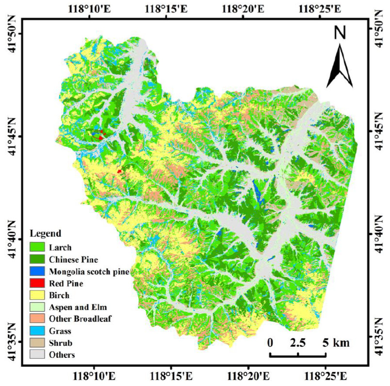
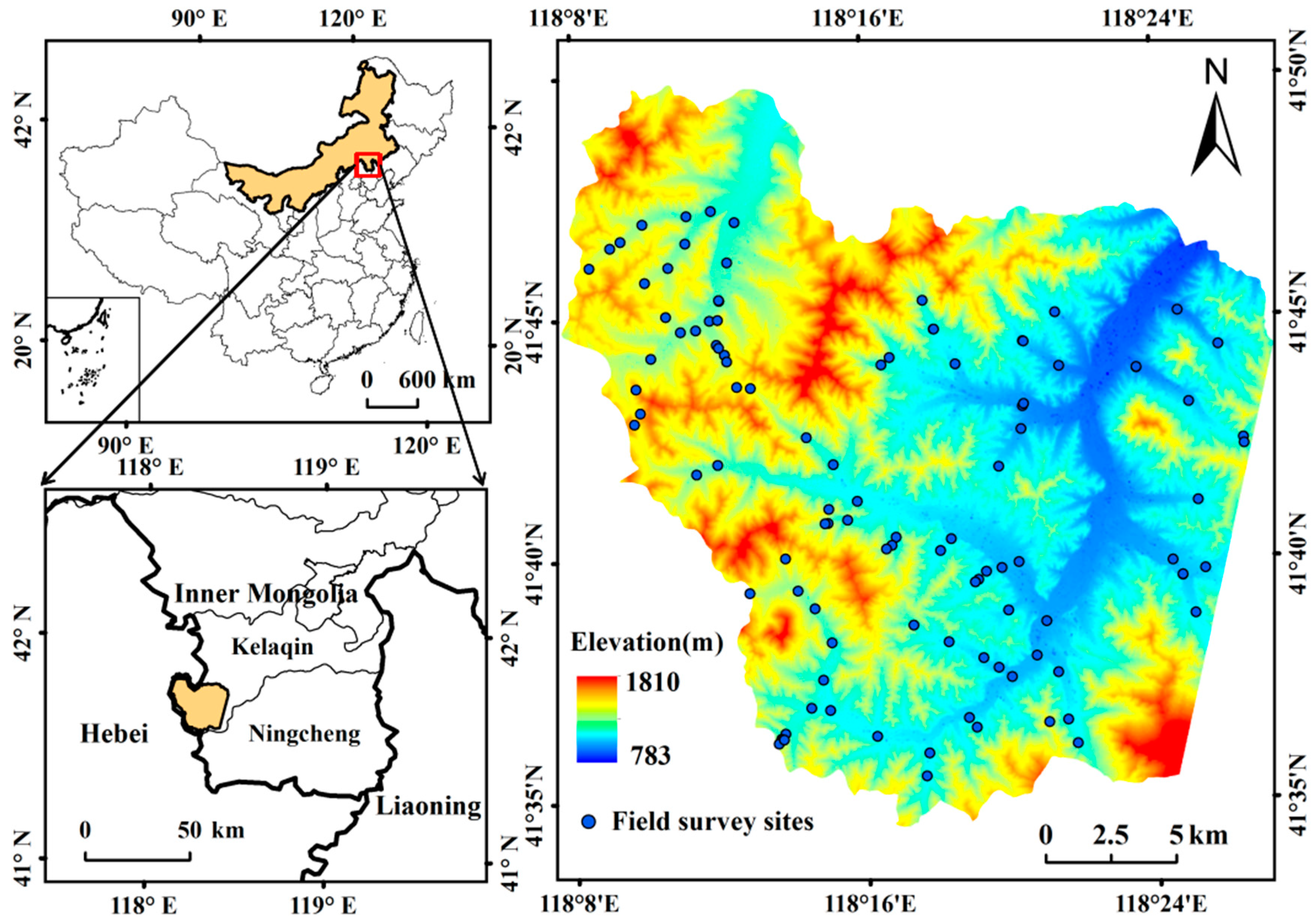
2.1. Study Area
2.2. Data Preparation
2.2.1. Field Survey Data Collection
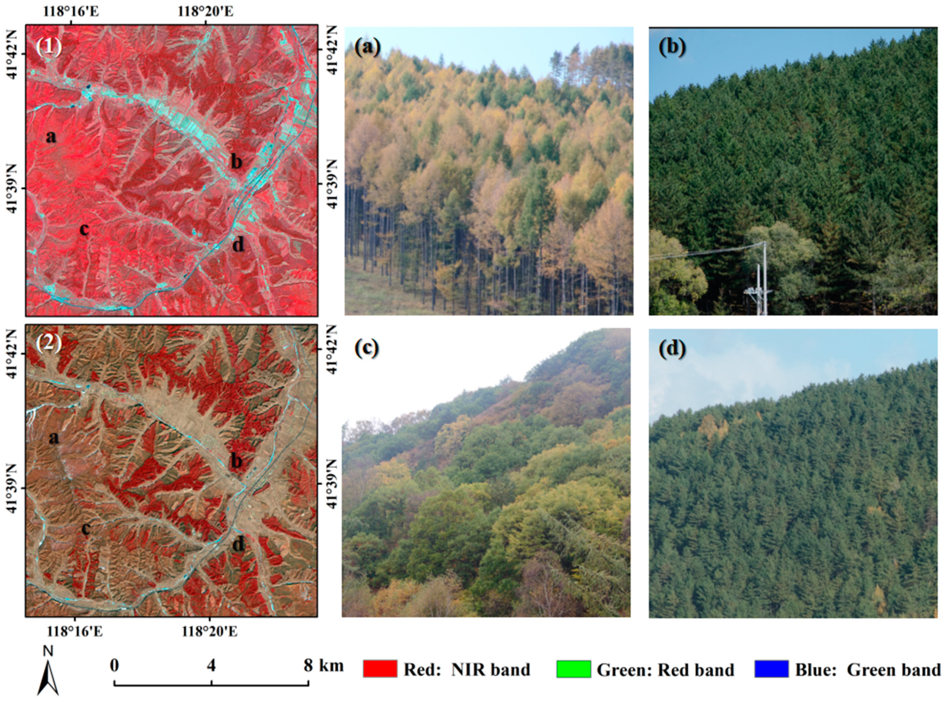
2.2.2. ZiYuan-3 Satellite Data Collection and Pre-Processing
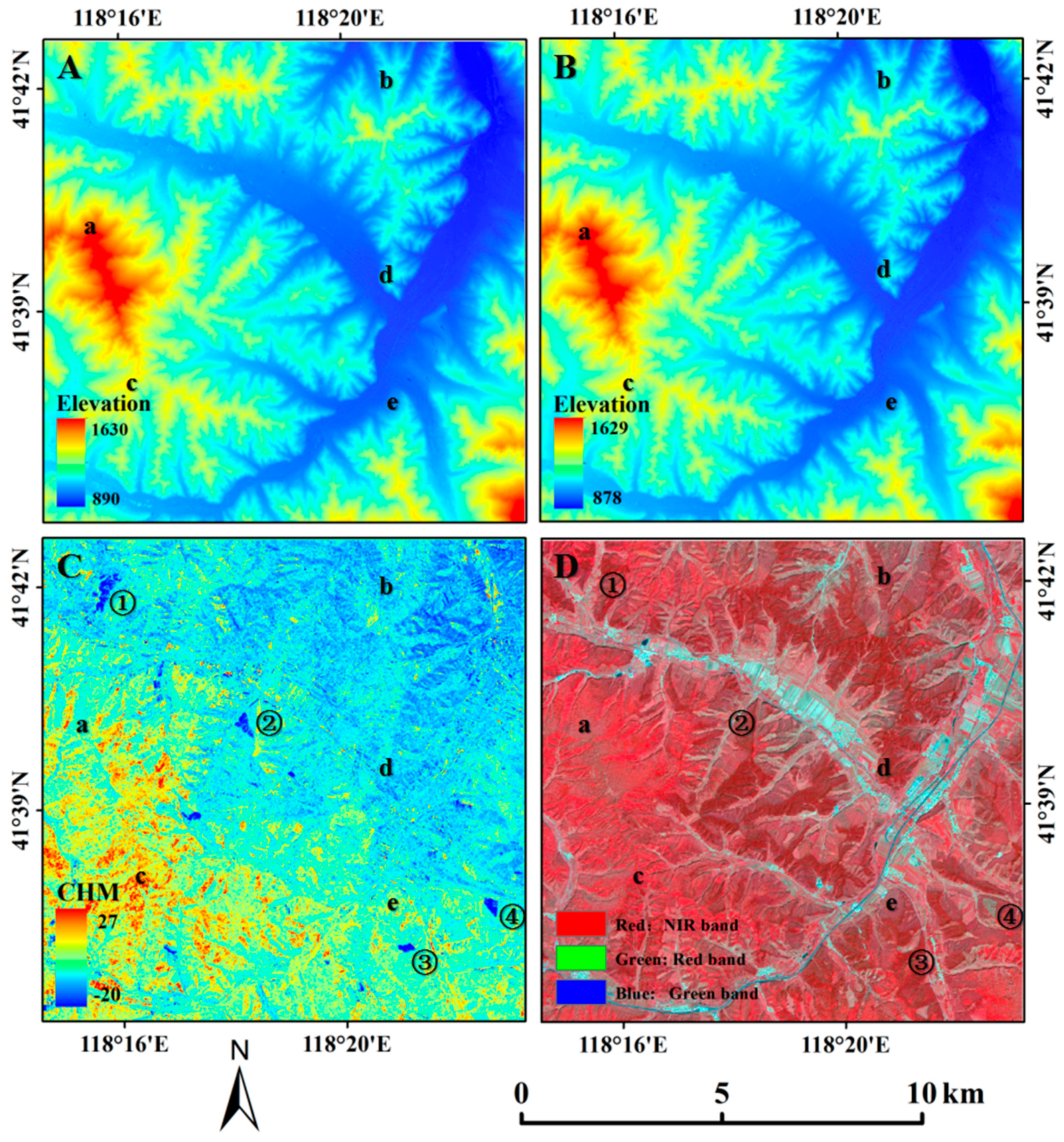
2.2.3. Development of Digital Surface Model Data from Stereo Images
2.2.4. Development of the Segment Image
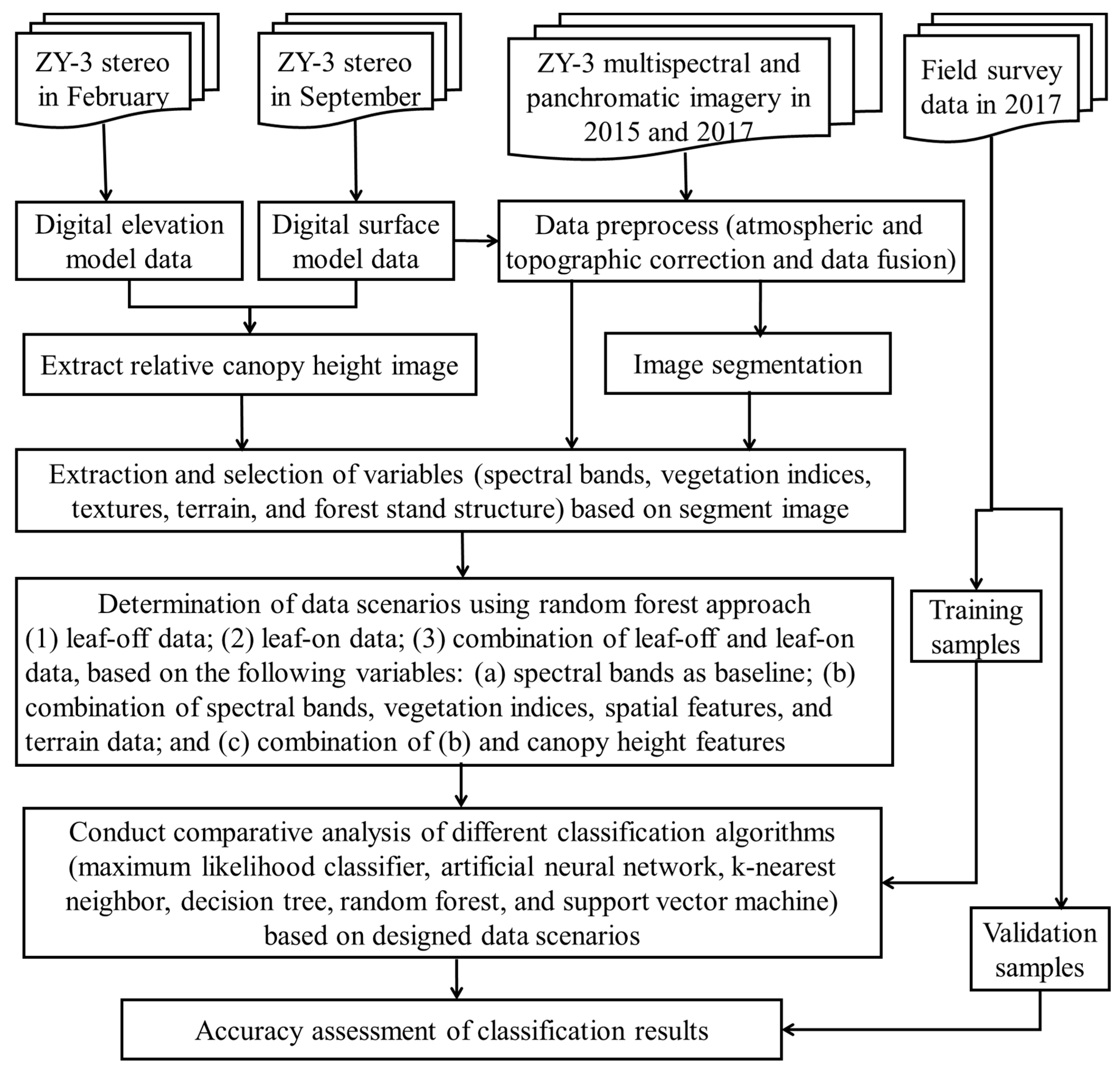
2.2.5. Framework of This Research
2.3. Extraction of Potential Variables and Selection of Optimal Variable Combination
2.3.1. Extraction of Spectral-Based Variables
2.3.2. Extraction of Spatial-Based Variables
2.3.3. Extraction of Forest Stand Based Variables
2.3.4. Extraction of Topographical-Based Variables
2.3.5. Selection of Suitable Variables Using Random Forest
2.4. Comparative Analysis of Classification Algorithms
2.4.1. A Brief Description of Six Classification Approaches
2.4.2. Comparative Analysis of Classification Results
3. Results
3.1. Comparative Analysis of Classification Results Based on Overall Land-Cover and Forest Types
3.1.1. Classification Results Based on Overall Land Cover Classes
3.1.2. Classification Results Based on Overall Forest Classes
3.1.3. Synthetic Analysis of Classification Results
3.2. Comparative Analysis of Classification Results Based on Tree Species
4. Discussion
4.1. Use of Seasonal Information to Improve Forest Classification Accuracy
4.2. The Roles of Spatial and Topographic Features
4.3. The Role of Canopy Height Features
4.4. Selection of a Suitable Classification Algorithm
4.5. The Need to Develop a Comprehensive Procedure for Forest Classification
5. Conclusions
- (1)
- If only spectral bands are used, MLC provides better land-cover or forest classification results than machine learning algorithms. MLC based on the combination of leaf-on and leaf-off spectral data can produce overall land cover classification of 76.4% and overall forest classification of 88.2% compared with the best results from machine learning algorithm with 72.9% for overall land covers and 76.1% for forest classes.
- (2)
- A leaf-off season image provides better classification results than a leaf-on image, and the combination of leaf-on and leaf-off images considerably improves the classification accuracy. The combination of leaf-on and leaf-off images can improve land cover classification accuracy by 15% and forest classification by 11.8%, which implies the necessity of using bi-temporal images for land cover or forest classification in the temperate climate zones.
- (3)
- Comparing only spectral bands, incorporation of multi-source data such as spectral responses, textures, and topographic factors can considerably improve classification, especially when machine learning algorithms such as RF and SVM are used. The overall land cover classification accuracy can be improved by 15.5% and forest by 12.7% using multiple source data compared to using spectral data alone, which implies the necessity of using multiple source data in land cover or forest classification in mountainous regions.
- (4)
- The addition of canopy height features may or may not improve forest classification, but can improve it for some tree species such as birch in leaf-off season and MSP in the leaf-on season. As accurate canopy height image can be extracted from lidar or from the combination of lidar and satellite stereo images, effective incorporation of canopy height features that can represent the difference of forest stand structures among different forest types into remotely sensed data will be a new research topic in improving forest classification.
- (5)
- Considering overall land-cover classification, RF and SVM provided the best classification accuracy of about 84%. Considering the overall forest classification, MLC provided the best accuracy of more than 89%, which is followed by RF and SVM with overall accuracy of more than 88%. Considering single tree species including larch, birch, and AAE had relatively lower classification accuracies than CP, MSP, RP, and OBL, and no single classification algorithm or data source provided the best accuracy for all tree species. This research implies the requirement to develop a comprehensive classification procedure that can employ specific approaches corresponding to different tree species. As high-performance computers and large volumes of different source data become available, deep learning approaches may be the new research directions for accurately mapping tree species distribution.
Author Contributions
Funding
Acknowledgments
Conflicts of Interest
References
- Brockerhoff, E.G.; Jactel, H.; Parrotta, J.A.; Quine, C.P.; Sayer, J. Plantation forests and biodiversity: Oxymoron or opportunity? Biodivers. Conserv. 2008, 17, 925–951. [Google Scholar] [CrossRef]
- Shang, X.; Chisholm, L.A. Classification of Australian native forest species using hyperspectral remote sensing and machine-learning classification algorithms. IEEE J.-STARS 2014, 7, 2481–2489. [Google Scholar] [CrossRef]
- Zhao, P.; Lu, D.; Wang, G.; Wu, C.; Huang, Y. Examining spectral reflectance saturation in Landsat imagery and corresponding solutions to improve forest aboveground biomass estimation. Remote Sens. 2016, 8. [Google Scholar] [CrossRef]
- Feng, Y.; Lu, D.; Chen, Q.; Keller, M.; Moran, E.; Dos-Santos, M.N.; Bolfe, E.L.; Batistella, M. Examining effective use of data sources and modeling algorithms for improving biomass estimation in a moist tropical forest of the Brazilian Amazon. Int. J. Digit. Earth 2017, 10, 996–1016. [Google Scholar] [CrossRef]
- Tao, B.; Tian, H.; Chen, G.; Ren, W.; Lu, C.; Alley, K.D.; Xu, X.; Liu, M.; Pan, S.; Virji, H. Terrestrial carbon balance in tropical Asia: Contribution from cropland expansion and land management. Glob. Planet. Chang. 2013, 100, 85–98. [Google Scholar] [CrossRef]
- Ray, D.; Bathgate, S.; Moseley, D.; Taylor, P.; Nicoll, B.; Pizzirani, S.; Gardiner, B. Comparing the provision of ecosystem services in plantation forests under alternative climate change adaptation management options in Wales. Reg. Environ. Chang. 2015, 15, 1501–1513. [Google Scholar] [CrossRef]
- D’Amato, D.; Rekola, M.; Wan, M.; Cai, D.; Toppinen, A. Effects of industrial plantations on ecosystem services and livelihoods: Perspectives of rural communities in China. Land Use Policy 2017, 63, 266–278. [Google Scholar] [CrossRef]
- Xiao, X.; Boles, S.; Liu, J.; Zhuang, D.; Liu, M. Characterization of forest types in Northeastern China, using multi-temporal SPOT-4 VEGETATION sensor data. Remote Sens. Environ. 2002, 82, 335–348. [Google Scholar] [CrossRef] [Green Version]
- Lin, C. China Forest Bureau announced the results of the fifth national forest resource inventory. Sci. Silv. Sin. 2000, 36, 105. [Google Scholar]
- China Forest Bureau. China Forest Resource Report (2008–2013); China Forestry Publishing House: Beijing, China, 2014; ISBN 9787503874246.
- Alatorre, L.C.; Sánchezandrés, R.; Cirujano, S.; Beguería, S.; Sánchezcarrillo, S. Identification of mangrove areas by remote sensing: The ROC curve technique applied to the northwestern Mexico coastal zone using Landsat imagery. Remote Sens. 2011, 3, 1568–1583. [Google Scholar] [CrossRef]
- Kempeneers, P.; Sedano, F.; Seebach, L.; Strobl, P.; San-Miguel-Ayanz, J. Data fusion of different spatial resolution remote sensing images applied to forest-type mapping. IEEE Trans. Geosci. Remote 2011, 49, 4977–4986. [Google Scholar] [CrossRef]
- Zhang, Y.; Lu, D.; Yang, B.; Sun, C.; Sun, M. Coastal wetland vegetation classification with a Landsat Thematic Mapper image. Int. J. Remote Sens. 2011, 32, 545–561. [Google Scholar] [CrossRef]
- Han, X.; Chen, X.; Feng, L. Four decades of winter wetland changes in Poyang Lake based on Landsat observations between 1973 and 2013. Remote Sens. Environ. 2015, 156, 426–437. [Google Scholar] [CrossRef]
- Dong, J.; Xiao, X.; Chen, B.; Torbick, N.; Jin, C.; Zhang, G.; Biradar, C. Mapping deciduous rubber plantations through integration of PALSAR and multi-temporal Landsat imagery. Remote Sens. Environ. 2013, 134, 392–402. [Google Scholar] [CrossRef]
- Qiao, H.; Wu, M.; Shakir, M.; Wang, L.; Kang, J.; Zheng, N. Classification of small-scale eucalyptus plantations based on NDVI time series obtained from multiple high-resolution datasets. Remote Sens. 2016, 8, 117. [Google Scholar] [CrossRef]
- Gomez, C.; Mangeas, M.; Petit, M.; Corbane, C.; Hamon, P. Use of high-resolution satellite imagery in an integrated model to predict the distribution of shade coffee tree hybrid zones. Remote Sens. Environ. 2010, 114, 2731–2744. [Google Scholar] [CrossRef]
- Han, N.; Wang, K.; Yu, L.; Zhang, X. Integration of texture and landscape features into object-based classification for delineating Torreya using IKONOS imagery. Int. J. Remote Sens. 2012, 33, 2003–2033. [Google Scholar] [CrossRef]
- Li, N.; Lu, D.; Wu, M.; Zhang, Y.; Lu, L. Coastal wetland classification with multiseasonal high-spatial resolution satellite imagery. Int. J. Remote Sens. 2018. [Google Scholar] [CrossRef]
- Xi, Z.; Lu, D.; Liu, L.; Ge, H. Detection of drought-induced hickory disturbances in western Lin’An county, China, using multitemporal Landsat imagery. Remote Sens. 2016, 8. [Google Scholar] [CrossRef]
- Lu, D.; Hetrick, S.; Moran, E. Land cover classification in a complex urban-rural Landscape with QuickBird imagery. Photogramm. Eng. Remote Sens. 2010, 76, 1159–1168. [Google Scholar] [CrossRef]
- Johnson, B.; Xie, Z. Classifying a high resolution image of an urban area using super-object information. ISPRS J. Photogramm. 2013, 83, 40–49. [Google Scholar] [CrossRef]
- Feng, Y.; Lu, D.; Moran, E.; Dutra, L.; Calvi, M.; De Oliveira, M. Examining spatial distribution and dynamic change of urban land covers in the Brazilian Amazon using multitemporal multisensor high spatial resolution satellite imagery. Remote Sens. 2017, 9, 381. [Google Scholar] [CrossRef]
- Cho, M.A.; Malahlela, O.; Ramoelo, A. Assessing the utility WorldView-2 imagery for tree species mapping in South African subtropical humid forest and the conservation implications: Dukuduku forest patch as case study. Int. J. Appl. Earth Obs. 2015, 38, 349–357. [Google Scholar] [CrossRef]
- Wang, Y.; Lu, D. Mapping Torreya grandis spatial distribution using high spatial resolution satellite imagery with the expert rules-based approach. Remote Sens. 2017, 9. [Google Scholar] [CrossRef]
- Reis, S.; Taşdemir, K. Identification of hazelnut fields using spectral and Gabor textural features. ISPRS J. Photogramm. 2011, 66, 652–661. [Google Scholar] [CrossRef]
- Lu, D.; Weng, Q. A survey of image classification methods and techniques for improving classification performance. Int. J. Remote Sens. 2007, 28, 823–870. [Google Scholar] [CrossRef] [Green Version]
- Lu, D.; Li, G.; Moran, E.; Dutra, L.; Batistella, M. The roles of textural images in improving land-cover classification in the Brazilian Amazon. Int. J. Remote Sens. 2014, 35, 8188–8207. [Google Scholar] [CrossRef]
- Immitzer, M.; Atzberger, C.; Koukal, T. Tree species classification with random forest using very high spatial resolution 8-band WorldView-2 satellite data. Remote Sens. 2012, 4, 2661–2693. [Google Scholar] [CrossRef]
- Zhang, X.; Du, S. Learning selfhood scales for urban land cover mapping with very-high-resolution satellite images. Remote Sens. Environ. 2016, 178, 172–190. [Google Scholar] [CrossRef]
- Dihkan, M.; Guneroglu, N.; Karsli, F.; Guneroglu, A. Remote sensing of tea plantations using an SVM classifier and pattern-based accuracy assessment technique. Int. J. Remote Sens. 2013, 34, 8549–8565. [Google Scholar] [CrossRef]
- Lu, D.; Moran, E.; Batistella, M. Linear mixture model applied to Amazonian vegetation classification. Remote Sens. Environ. 2003, 87, 456–469. [Google Scholar] [CrossRef] [Green Version]
- Lu, D. Integration of vegetation inventory data and Landsat TM image for vegetation classification in the western Brazilian Amazon. For. Ecol. Manag. 2005, 213, 369–383. [Google Scholar] [CrossRef]
- Holmgren, J.; Persson, Å.; Söderman, U. Species identification of individual trees by combining high resolution LiDAR data with multi-spectral images. Int. J. Remote Sens. 2008, 29, 1537–1552. [Google Scholar] [CrossRef]
- Eetu, P.; Juha, S.; Teemu, H.; Esa, R.; Harri, K.; Sanna, K.; Paula, L. Tree species classification from fused active hyperspectral reflectance and LIDAR measurements. For. Ecol. Manag. 2010, 260, 1843–1852. [Google Scholar] [CrossRef]
- Ke, Y.; Quackenbush, L.J.; Im, J. Synergistic use of QuickBird multispectral imagery and LIDAR data for object-based forest species classification. Remote Sens. Environ. 2010, 114, 1141–1154. [Google Scholar] [CrossRef]
- Dalponte, M.; Bruzzone, L.; Gianelle, D. Tree species classification in the Southern Alps based on the fusion of very high geometrical resolution multispectral/hyperspectral images and LiDAR data. Remote Sens. Environ. 2012, 123, 258–270. [Google Scholar] [CrossRef]
- Haby, N.; Tunn, Y.; Cameron, J. Application of QuickBird and aerial imagery to detect Pinus radiata in remnant vegetation. Aust. Ecol. 2010, 35, 624–635. [Google Scholar] [CrossRef]
- Ferreira, M.P.; Zortea, M.; Zanotta, D.C.; Shimabukuro, Y.E. Mapping tree species in tropical seasonal semi-deciduous forests with hyperspectral and multispectral data. Remote Sens. Environ. 2016, 179, 66–78. [Google Scholar] [CrossRef]
- Dalponte, M.; Orka, H.O.; Gobakken, T.; Gianelle, D.; Naesset, E. Tree species classification in boreal forests with hyperspectral data. IEEE Trans. Geosci. Remote 2013, 51, 2632–2645. [Google Scholar] [CrossRef]
- Raczko, E.; Zagajewski, B. Comparison of support vector machine, random forest and neural network classifiers for tree species classification on airborne hyperspectral APEX images. Eur. J. Remote Sens. 2017, 50, 144–154. [Google Scholar] [CrossRef]
- Chen, Y.; Lin, Z.; Zhao, X.; Wang, G.; Gu, Y. Deep learning-based classification of hyperspectral data. IEEE J.-STARS 2017, 7, 2094–2107. [Google Scholar] [CrossRef]
- Pan, B.; Shi, Z.; Xu, X. MugNet: Deep learning for hyperspectral image classification using limited samples. ISPRS J. Photogramm. 2017. [Google Scholar] [CrossRef]
- Zou, X.; Cheng, M.; Wang, C.; Xia, Y.; Li, J. Tree classification in complex forest point clouds based on deep learning. IEEE Geosci. Remote 2017, 14, 2360–2364. [Google Scholar] [CrossRef]
- Feng, Z.; Xie, M.; Gao, Y. Evaluation on the woodland resource value in Wangyedian trial forest farm. For. Invent. Plan. 2014, 29, 60–65. [Google Scholar]
- Zhang, N.; Feng, Z.; Feng, Y.; Fan, J. Research on coniferous forest volume estimation model for Wangyedian experimental forest farm. J. Cent. South Univ. For. Technol. 2013, 33, 83–87. [Google Scholar]
- Gong, Y.; He, C.; Yan, F.; Feng, Z.; Cao, M.; Gao, Y.; Miao, J.; Zhao, J. Study on artificial neural network combined with multispectral remote sensing imagery for forest site evaluation. Spectrosc. Spect. Anal. 2013, 33, 2815–2822. [Google Scholar] [CrossRef]
- Wu, G. Wangyedian forest farm operates. J. Inner Mongol. For. 1989, 1, 11. [Google Scholar]
- Wu, C.; Ma, C. Struggle for sixty years, dream and flourishing industry—Record of development of Wangye Dian Experimental Forest Farm in Chifeng, the Inner Mongolia Autonomous Region. Land Green. 2015, 7, 16–19. [Google Scholar]
- Li, X.; Chen, W.; Cheng, X. A comparison of machine learning algorithms for mapping of complex surface-mined and agricultural landscapes using ZiYuan-3 stereo satellite imagery. Remote Sens. 2016, 8, 514. [Google Scholar] [CrossRef]
- Luo, H.; Li, L.; Zhu, H.; Kuai, X.; Zhang, Z.; Liu, Y. Land cover extraction from high resolution ZY-3 satellite imagery using ontology-based method. ISPRS Int. J. Geo-Inf. 2016, 5, 31. [Google Scholar] [CrossRef]
- Gu, H.; Li, H.; Yan, L.; Liu, Z.; Blaschke, T.; Soergel, U. An object-based semantic classification method for high resolution remote sensing imagery using ontology. Remote Sens. 2017, 9, 329. [Google Scholar] [CrossRef]
- Chander, G.; Markham, B.L.; Helder, D.L. Summary of current radiometric calibration coefficients for Landsat MSS, TM, ETM+, and EO-1 ALI sensors. Remote Sens. Environ. 2009, 113, 893–903. [Google Scholar] [CrossRef] [Green Version]
- Gao, M.; Zhao, W.; Gong, Z.; Chen, Z.; Tang, X. Topographic correction of ZY-3 satellite images and its effects on estimation of shrub leaf biomass in mountainous areas. Remote Sens. 2014, 6, 3141–3151. [Google Scholar] [CrossRef]
- Reese, H.; Olsson, H. C-correction of optical satellite data over alpine vegetation areas: A comparison of sampling strategies for determining the empirical c-parameter. Remote Sens. Environ. 2011, 115, 1387–1400. [Google Scholar] [CrossRef] [Green Version]
- Sola, I.; González-Audícana, M.; Álvarez-Mozos, J. Multi-criteria evaluation of topographic correction methods. Remote Sens. Environ. 2011, 184, 247–262. [Google Scholar] [CrossRef]
- Karathanassi, V.; Kolokousis, P.; Ioannidou, S. A comparison study on fusion methods using evaluation indicators. Int. J. Remote Sens. 2007, 28, 2309–2341. [Google Scholar] [CrossRef]
- Zhang, J. Multi-source remote sensing data fusion: Status and trends. Int. J. Image Data Fusion 2010, 1, 5–24. [Google Scholar] [CrossRef]
- Ni, W.; Sun, G.; Ranson, K.J.; Pang, Y.; Zhang, Z.; Yao, W. Extraction of ground surface elevation from ZY-3 winter stereo imagery over deciduous forested areas. Remote Sens. Environ. 2015, 159, 194–202. [Google Scholar] [CrossRef]
- Hirano, A.; Welch, R.; Lang, H. Mapping from ASTER stereo image data: DEM validation and accuracy assessment. ISPRS J. Photogramm. 2003, 57, 356–370. [Google Scholar] [CrossRef]
- Sefercik, U.G.; Alkan, M.; Buyuksalih, G.; Jacobsen, K. Generation and validation of high-resolution DEMs from Worldview-2 stereo data. Photogramm. Rec. 2013, 28, 362–374. [Google Scholar] [CrossRef]
- Krishnan, S.; Sajikumar, N.; Sumam, K.S. DEM generation using Cartosat-I stereo data and its comparison with publically available DEM. Procedia Technol. 2016, 24, 295–302. [Google Scholar] [CrossRef]
- Lu, D.; Mausel, P.; Batistella, M.; Moran, E. Comparison of land-cover classification methods in the Brazilian Amazon Basin. Photogramm. Eng. Remote Sens. 2004, 70, 723–732. [Google Scholar] [CrossRef]
- Li, G.; Lu, D.; Moran, E.; Sant’Anna, S.J.S. A comparative analysis of classification algorithms and multiple sensor data for land use/land cover classification in the Brazilian Amazon. J. Appl. Remote Sens. 2012, 6, 061706. [Google Scholar] [CrossRef]
- Bannari, A.; Morin, D.; Bonn, F.; Huete, A.R. A review of vegetation indices. Remote Sens. Rev. 1995, 13, 95–120. [Google Scholar] [CrossRef]
- Baugh, W.M.; Groeneveld, D.P. Broadband vegetation index performance evaluated for a low-cover environment. Int. J. Remote Sens. 2006, 27, 4715–4730. [Google Scholar] [CrossRef]
- Louhaichi, M.; Borman, M.; Johnson, D. Spatially located platform and aerial photography for documentation of grazing impacts on wheat. Geocarto Int. 2001, 16, 65–70. [Google Scholar] [CrossRef]
- Wang, X.; Wang, M.; Wang, S.; Wu, Y. Extraction of vegetation information from visible unmanned aerial vehicle images. Trans. Chin. Soc. Agric. Eng. 2015, 31, 152–159. [Google Scholar] [CrossRef]
- Haralick, R.M.; Shanmugam, K.; Dinstein, I.H. Textural features for image classification. IEEE Trans. Syst. Man Cycle 1973, 3, 610–621. [Google Scholar] [CrossRef]
- Yu, Q.; Gong, P.; Clinton, N.; Biging, G.; Kelly, M.; Schirokauer, D. Object-based detailed vegetation classification with airborne high spatial resolution remote sensing imagery. Photogramm. Eng. Remote Sens. 2006, 72, 799–811. [Google Scholar] [CrossRef]
- Jiao, L.; Liu, Y.; Li, H. Characterizing land-use classes in remote sensing imagery by shape metrics. ISPRS J. Photogramm. 2012, 72, 46–55. [Google Scholar] [CrossRef]
- Fassnacht, F.E.; Latifi, H.; Sterenczak, K.; Modzelewska, A.; Lefsky, M.; Waser, L.T.; Straub, C.; Ghosh, A. Review of studies on tree species classification from remotely sensed data. Remote Sens. Environ. 2016, 186, 64–87. [Google Scholar] [CrossRef]
- Keuchel, J.; Naumann, S.; Heiler, M.; Siegmund, A. Automatic land cover analysis for Tenerife by supervised classification using remotely sensed data. Remote Sens. Environ. 2003, 86, 530–541. [Google Scholar] [CrossRef]
- Tso, B.; Mather, P.M. Classification Methods for Remotely Sensed Data; Taylor and Francis Inc.: New York, NY, USA, 2001. [Google Scholar]
- Kimes, D.S.; Nelson, R.F.; Manry, M.T.; Fung, A.K. Attributes of neural networks for extracting continuous vegetation variables from optical and radar measurements. Int. J. Remote Sens. 1998, 19, 2639–2663. [Google Scholar] [CrossRef]
- Gong, P.; Pu, R.; Yu, B. Conifer species recognition: An exploratory analysis of in situ hyperspectral data. Remote Sens. Environ. 1997, 62, 189–200. [Google Scholar] [CrossRef]
- Cortijo, F.J.; Blanca, P.D.L. A comparative study of some non-parametric spectral classifiers. Applications to problems with high-overlapping training sets. Int. J. Remote Sens. 1997, 18, 1259–1275. [Google Scholar] [CrossRef]
- Collions, M.J.; Dymond, C.; Johnson, E.A. Mapping subalpine forest types using networks of nearest neighbor classifiers. Int. J. Remote Sens. 2004, 25, 1701–1721. [Google Scholar] [CrossRef]
- Haapanen, R.; Ek, A.R.; Bauer, M.E.; Finley, A.O. Delineation of forest/nonforest land use classes using nearest neighbor methods. Remote Sens. Environ. 2004, 89, 265–271. [Google Scholar] [CrossRef]
- Lu, D.; Li, G.; Moran, E.; Kuang, W. A comparative analysis of approaches for successional vegetation classification in the Brazilian Amazon. Gisci. Remote Sens. 2014, 51, 695–709. [Google Scholar] [CrossRef]
- Quinlan, J.R. Induction of Decision Trees. Mach. Learn. 1986, 1, 81–106. [Google Scholar] [CrossRef]
- Landgrebe, D. A survey of decision tree classifier methodology. IEEE Trans. Syst. Man Cycle 1991, 21, 660–674. [Google Scholar] [CrossRef] [Green Version]
- Friedl, M.A.; Brodley, C.E. Decision tree classification of land cover from remotely sensed data. Remote Sens. Environ. 1997, 61, 399–409. [Google Scholar] [CrossRef]
- Osei-Bryson, K.M. Post-pruning in decision tree induction using multiple performance measures. Comput. Oper. Res. 2007, 34, 3331–3345. [Google Scholar] [CrossRef]
- Fürnkranz, J. Pruning algorithms for rule learning. Mach. Learn. 1997, 27, 139–172. [Google Scholar] [CrossRef]
- Hansen, M.; Dubayah, R.; DeFries, R. Classification trees: An alternative to traditional land cover classifiers. Int. J. Remote Sens. 1996, 17, 1075–1081. [Google Scholar] [CrossRef]
- Lawrence, R.; Bunn, A.; Powell, S.; Zambon, M. Classification of remotely sensed imagery using stochastic gradient boosting as a refinement of classification tree analysis. Remote Sens. Environ. 2004, 90, 331–336. [Google Scholar] [CrossRef]
- Breiman, L. Bagging predictors. Mach. Learn. 1996, 24, 123–140. [Google Scholar] [CrossRef] [Green Version]
- Breiman, L. Random Forests. Mach. Learn. 2001, 45, 5–32. [Google Scholar] [CrossRef] [Green Version]
- Stumpf, A.; Kerle, N. Object-oriented mapping of landslides using Random Forests. Remote Sens. Environ. 2011, 115, 2564–2577. [Google Scholar] [CrossRef]
- Brown, M.; Gunn, S.R.; Lewis, H.G. Support vector machines for optimal classification and spectral unmixing. Ecol. Model. 1999, 120, 167–179. [Google Scholar] [CrossRef]
- Wang, S.; Meng, B. Parameter selection algorithm for support vector machine. Procedia Environ. Sci. 2011, 11, 538–544. [Google Scholar] [CrossRef]
- Hearst, M.A.; Dumais, S.T.; Osuna, E.; Platt, J.; Scholkopf, B. Support vector machines. IEEE Intell. Syst. Their Appl. 1998, 13, 18–28. [Google Scholar] [CrossRef]
- Brereton, R.G.; Lloyd, G.R. Support vector machines for classification and regression. Analyst 2010, 135, 230–267. [Google Scholar] [CrossRef]
- Foody, G.M. Status of land cover classification accuracy assessment. Remote Sens. Environ. 2002, 80, 185–201. [Google Scholar] [CrossRef]
- Congalton, R.G.; Green, K. Assessing the Accuracy of Remotely Sensed Data: Principles and Practices, 2nd ed.; CRC Press: Boca Raton, FL, USA, 2008. [Google Scholar]
- Liu, C.; Frazier, P.; Kumar, L. Comparative assessment of the measures of thematic classification accuracy. Remote Sens. Environ. 2007, 107, 606–616. [Google Scholar] [CrossRef]
- Liu, Q.J.; Takamura, T.; Takeuchi, N.; Shao, G. Mapping of boreal vegetation of a temperate mountain in China by multitemporal Landsat TM imagery. Int. J. Remote Sens. 2002, 23, 3385–3405. [Google Scholar] [CrossRef]
- Cho, M.A.; Mathieu, R.; Asner, G.P.; Naidoo, L.; Aardt, J.; Ramoelo, A.; Debba, P.; Wessels, K.; Main, R.; Smit, I.P.J.; et al. Mapping tree species composition in South African savannas using an integrated airborne spectral and LiDAR system. Remote Sens. Environ. 2012, 125, 214–226. [Google Scholar] [CrossRef]
- Franklin, S.E.; Hall, R.J.; Moskal, L.M.; Maudie, A.J.; Lavigne, M.B. Incorporating texture into classification of forest species composition from airborne multispectral images. Int. J. Remote Sens. 2000, 21, 61–79. [Google Scholar] [CrossRef]
- Wessel, M.; Brandmeier, M.; Tiede, D. Evaluation of different machine learning algorithms for scalable classification of tree types and tree species based on Sentinel-2 data. Remote Sens. 2018, 10, 1419. [Google Scholar] [CrossRef]
- Blaschke, T.; Burnett, C.; Pekkarinen, A. Image segmentation methods for object-based analysis and classification. In Remote Sensing Image Analysis: Including the Spatial Domain; de Jong, S.M., van der Meer, F.D., Eds.; Kluwer Academic Publishers: Dordrecht, The Netherlands, 2004; pp. 211–236. [Google Scholar]
- Myint, S.W.; Gober, P.; Brazel, A.; Grossman-Clarke, S.; Weng, Q. Per-pixel vs object-based classification of urban land cover extraction using high spatial resolution imagery. Remote Sens. Environ. 2011, 115, 1145–1161. [Google Scholar] [CrossRef]
- Wang, D.; Wan, B.; Qiu, P.; Su, Y.; Guo, Q.; Wu, X. Artificial mangrove species mapping using Pléiades-1: An evaluation of pixel-based and object-based classifications with selected machine learning algorithms. Remote Sens. 2018, 10, 294. [Google Scholar] [CrossRef]
- Gao, Y.; Mas, J.F.; Maathuis, B.H.P.; Zhang, X.; Van Dijk, P.M. Comparison of pixel-based and object-oriented image classification approaches—A case study in a Coal Fire Area, Wuda, Inner Mongolia, China. Int. J. Remote Sens. 2006, 27, 4039–4055. [Google Scholar] [CrossRef]
- Zhang, C.; Xie, Z. Combining object-based texture measures with a neural network for vegetation mapping in the everglades from hyperspectral imagery. Remote Sens. Environ. 2012, 124, 310–320. [Google Scholar] [CrossRef]
- Han, N.; Du, H.; Zhou, G.; Sun, X.; Ge, H.; Xu, X. Object-based classification using SPOT-5 imagery for Moso bamboo forest mapping. Int. J. Remote Sens. 2014, 35, 1126–1142. [Google Scholar] [CrossRef]


| Data | Data Description | Data Acquisition Dates |
|---|---|---|
| Field survey data | A total of 112 sites were investigated, for which all land covers around each site were recorded, digitized, and saved in a shape file format. Thus, over 1000 samples covering different land covers were collected. | September 2017 |
| ZiYuan-3 satellite data | Four multispectral bands (blue, green, red, and near infrared (NIR)): 5.8 m spatial resolution; One panchromatic band: 2 m spatial resolution; Stereo images: nadir-view image with 2 m, backward and forward views with 3.5 m spatial resolution | 9 February 2015: sun elevation angle of 31.44° and azimuth angle of 163.06°; 20 September 2017: sun elevation angle of 44.22° and azimuth angle of 148.18° |
| Vegetation Indices | Equations | References |
|---|---|---|
| Differenced vegetation index (DVI) | NIR − Red | [65] |
| Infrared percentage vegetation index (IPVI) | NIR/(NIR + Red) | [66] |
| Normalized difference vegetation index (NDVI) | (NIR − Red)/(NIR + Red) | [65] |
| Normalized difference greenness index (NDGI) | (Green − Red)/(Green + Red) | [65] |
| Normalized difference water index (NDWI) | (Green − NIR)/(Green + NIR) | [65] |
| Ratio vegetation index (RVI) | NIR/Red | [25] |
| Re-normalized difference vegetation index (RDVI) | (NIR − Red)/ | [4] |
| Visible-band difference vegetation index (VDVI) | [67,68] | |
| Optimized soil adjusted vegetation index (OSAVI) | (NIR − Red)/(NIR + Red + 0.16) | [4] |
| Ratio of near-infrared (NIR) band to blue band | NIR/Blue | [25] |
| Data | Variables | |
|---|---|---|
| Data from leaf-off season | V1off | BlueF, GreenF, RedF, NIRF. |
| V2off | NDVIF, Brightness, NDGIF, Slope, NIRF, Elevation, TF-Cor-NIR, TF-Cor-Green, VDVIF, Aspect, TF-Hom-Red, TF-Hom-Blue, TF-Std-Red. | |
| V3off | NDVIF, RCH, Brightness, NDGIF, Slope, NIRF, Elevation, TF-Cor-NIR, TF-Cor-Green, VDVIF, TEnt-RCH, Aspect, TF-Hom-Red, TDis-RCH, TF-Hom-Blue, TF-Std-Red. | |
| Data from leaf-on season | V1on | BlueS, GreenS, RedS, NIRS. |
| V2on | SUMS-all-band, VDVIS, TS-Sec-Blue, NIR/SUMS-all-band, NIR/BLUES, NIRS, Elevation, TS-Std-Red, TS-Hom-NIR, NDGIS, Slope, TS-Dis-NIR, TS-Con-Red, TS-Ent-NIR, Length/Width. | |
| V3on | SUMS-all-band, VDVIS, TS-Sec-Blue, NIR/SUMS-all-band, NIR/BLUES, NIRS, Elevation, TS-Std-Red, TS-Hom-NIR, RCH, NDGIS, Slope, TS-Dis-NIR, TS-Con-Red, TSec-RCH, TS-Ent-NIR, Length/Width. | |
| Combined data from both seasons | V1both | BlueF, GreenF, RedF, NIRF, BlueS, GreenS, RedS, NIRS. |
| V2both | IPVIF, SUMS-all-band, IPVIS, VDVIS, NIRS, TS-Sec-Blue, NDGI (diff), NDGIS, TS-Hom-NIR, VDVI (diff), Slope, TS-Ent-Blue, VDVIF, Elevation, TS-Cor-Red, NDGIF, TS-Std-NIR. | |
| V3both | IPVIF, SUMS-all-band, IPVIS, VDVIS, NIRS, TS-Sec-Blue, NDGI (diff), NDGIS, RCH, TS-Hom-NIR, VDVI (diff), Slope, TS-Ent-Blue, VDVIF, Elevation, TS-Cor-Red, NDGIF, TS-Std-NIR. | |
| Samples | Number of Samples for Each Class | Total | ||||||||||||
|---|---|---|---|---|---|---|---|---|---|---|---|---|---|---|
| Larch | CP | MSP | RP | Birch | AAE | OBL | Shrub | Grass | FL | BL | Water | ISA | ||
| Training | 167 | 221 | 36 | 16 | 83 | 69 | 71 | 33 | 45 | 105 | 48 | 14 | 148 | 1056 |
| Validation | 58 | 95 | 31 | 30 | 59 | 43 | 52 | 53 | 68 | 85 | 47 | 30 | 31 | 682 |
| Data Scenarios | Overall Land-Cover Classification Accuracy (%) Based on Six Algorithms | ||||||
|---|---|---|---|---|---|---|---|
| MLC | ANN | kNN | DT | RF | SVM | ||
| Data from leaf-off season | V1off | 68.62 | 41.64 | 48.97 | 50.29 | 57.92 | 57.18 |
| V2off | 76.10 | 45.45 | 75.95 | 63.34 | 66.86 | 73.46 | |
| V3off | 76.10 | 47.36 | 58.06 | 64.37 | 67.16 | 74.49 | |
| Data from leaf-on season | V1on | 66.72 | 47.21 | 54.69 | 58.94 | 63.20 | 59.09 |
| V2on | 72.14 | 59.68 | 68.48 | 65.98 | 72.29 | 78.59 | |
| V3on | 73.02 | 54.84 | 70.09 | 69.94 | 77.27 | 78.89 | |
| Combined data from both seasons | V1both | 76.39 | 65.98 | 63.05 | 65.69 | 69.79 | 72.87 |
| V2both | 80.06 | 66.13 | 78.74 | 75.07 | 83.58 | 84.46 | |
| V3both | 78.59 | 61.88 | 79.03 | 72.29 | 83.14 | 82.99 | |
| Accuracy Assessment Results Based on V2off Data Using Support Vector Machine | |||||||||||||||
|---|---|---|---|---|---|---|---|---|---|---|---|---|---|---|---|
| Type | Larch | CP | MSP | RP | Birch | AAE | OBL | Shrub | Grass | FL | BL | Water | ISA | UA | PA |
| Larch | 51 | 0 | 0 | 0 | 6 | 0 | 3 | 5 | 3 | 1 | 2 | 0 | 0 | 71.8 | 87.9 |
| CP | 0 | 80 | 3 | 0 | 0 | 1 | 0 | 0 | 1 | 1 | 1 | 0 | 0 | 92.0 | 84.2 |
| MSP | 0 | 4 | 28 | 0 | 0 | 0 | 0 | 0 | 0 | 0 | 0 | 0 | 0 | 87.5 | 90.3 |
| RP | 0 | 8 | 0 | 30 | 0 | 0 | 0 | 0 | 0 | 0 | 0 | 0 | 0 | 79.0 | 100 |
| Birch | 0 | 3 | 0 | 0 | 50 | 0 | 8 | 1 | 5 | 0 | 1 | 0 | 0 | 73.5 | 84.7 |
| AAE | 1 | 0 | 0 | 0 | 0 | 36 | 0 | 1 | 4 | 6 | 1 | 0 | 1 | 72.0 | 83.7 |
| OBL | 2 | 0 | 0 | 0 | 2 | 0 | 39 | 4 | 7 | 0 | 1 | 0 | 0 | 70.9 | 75.0 |
| Shrub | 1 | 0 | 0 | 0 | 0 | 0 | 1 | 34 | 2 | 1 | 3 | 0 | 0 | 81.0 | 64.2 |
| Grass | 3 | 0 | 0 | 0 | 1 | 0 | 1 | 4 | 32 | 5 | 5 | 0 | 2 | 60.4 | 47.1 |
| FL | 0 | 0 | 0 | 0 | 0 | 3 | 0 | 2 | 6 | 56 | 5 | 1 | 2 | 74.7 | 65.9 |
| BL | 0 | 0 | 0 | 0 | 0 | 0 | 0 | 2 | 4 | 0 | 21 | 0 | 0 | 77.8 | 44.7 |
| Water | 0 | 0 | 0 | 0 | 0 | 0 | 0 | 0 | 0 | 0 | 2 | 18 | 0 | 90.0 | 60.0 |
| ISA | 0 | 0 | 0 | 0 | 0 | 3 | 0 | 0 | 4 | 15 | 5 | 11 | 26 | 40.6 | 83.9 |
| Accuracy assessment results based on V2on data using support vector machine | |||||||||||||||
| Larch | 47 | 8 | 2 | 0 | 7 | 1 | 0 | 6 | 2 | 0 | 0 | 0 | 0 | 64.4 | 81.0 |
| CP | 2 | 67 | 3 | 0 | 4 | 0 | 0 | 0 | 0 | 0 | 0 | 0 | 0 | 88.2 | 70.5 |
| MSP | 5 | 12 | 26 | 0 | 0 | 0 | 0 | 0 | 0 | 0 | 0 | 0 | 0 | 60.5 | 83.9 |
| RP | 0 | 1 | 0 | 30 | 0 | 0 | 0 | 0 | 0 | 0 | 0 | 0 | 0 | 96.8 | 100 |
| Birch | 2 | 2 | 0 | 0 | 47 | 0 | 5 | 2 | 2 | 0 | 0 | 0 | 0 | 78.3 | 79.7 |
| AAE | 0 | 4 | 0 | 0 | 0 | 39 | 0 | 0 | 1 | 3 | 0 | 3 | 0 | 78.0 | 90.7 |
| OBL | 0 | 0 | 0 | 0 | 1 | 0 | 47 | 0 | 0 | 0 | 0 | 0 | 0 | 97.9 | 90.4 |
| Shrub | 1 | 1 | 0 | 0 | 0 | 0 | 0 | 39 | 3 | 1 | 0 | 0 | 0 | 86.7 | 73.6 |
| Grass | 1 | 0 | 0 | 0 | 0 | 2 | 0 | 5 | 52 | 10 | 1 | 0 | 0 | 73.2 | 76.5 |
| FL | 0 | 0 | 0 | 0 | 0 | 0 | 0 | 1 | 2 | 56 | 7 | 0 | 0 | 84.9 | 65.9 |
| BL | 0 | 0 | 0 | 0 | 0 | 1 | 0 | 0 | 6 | 6 | 36 | 0 | 0 | 73.5 | 76.6 |
| Water | 0 | 0 | 0 | 0 | 0 | 0 | 0 | 0 | 0 | 1 | 0 | 19 | 0 | 95.0 | 63.3 |
| ISA | 0 | 0 | 0 | 0 | 0 | 0 | 0 | 0 | 0 | 8 | 3 | 8 | 31 | 62.0 | 100 |
| Accuracy assessment results based on V2both data using the support vector machine | |||||||||||||||
| Larch | 55 | 0 | 0 | 0 | 11 | 0 | 0 | 2 | 1 | 0 | 0 | 0 | 0 | 79.7 | 94.8 |
| CP | 0 | 74 | 2 | 0 | 0 | 0 | 0 | 0 | 0 | 0 | 0 | 0 | 0 | 97.4 | 77.9 |
| MSP | 0 | 8 | 29 | 0 | 0 | 0 | 0 | 0 | 0 | 0 | 0 | 0 | 0 | 78.4 | 93.6 |
| RP | 0 | 12 | 0 | 30 | 0 | 0 | 0 | 0 | 0 | 0 | 0 | 0 | 0 | 71.4 | 100 |
| Birch | 0 | 0 | 0 | 0 | 46 | 0 | 3 | 2 | 0 | 0 | 0 | 0 | 0 | 90.2 | 78.0 |
| AAE | 0 | 0 | 0 | 0 | 0 | 39 | 0 | 0 | 1 | 1 | 0 | 0 | 0 | 95.1 | 90.7 |
| OBL | 0 | 0 | 0 | 0 | 1 | 0 | 49 | 0 | 1 | 0 | 0 | 0 | 0 | 96.1 | 94.2 |
| Shrub | 1 | 1 | 0 | 0 | 1 | 0 | 0 | 38 | 2 | 1 | 1 | 0 | 0 | 84.4 | 71.7 |
| Grass | 2 | 0 | 0 | 0 | 0 | 1 | 0 | 5 | 52 | 6 | 0 | 1 | 0 | 77.6 | 76.5 |
| FL | 0 | 0 | 0 | 0 | 0 | 3 | 0 | 1 | 8 | 71 | 8 | 1 | 2 | 75.5 | 83.5 |
| BL | 0 | 0 | 0 | 0 | 0 | 0 | 0 | 5 | 3 | 6 | 37 | 1 | 0 | 71.2 | 78.7 |
| Water | 0 | 0 | 0 | 0 | 0 | 0 | 0 | 0 | 0 | 0 | 0 | 27 | 0 | 100.0 | 90.0 |
| ISA | 0 | 0 | 0 | 0 | 0 | 0 | 0 | 0 | 0 | 0 | 1 | 0 | 29 | 96.7 | 93.6 |
| Land-Cover Type | Area (km2) | % |
|---|---|---|
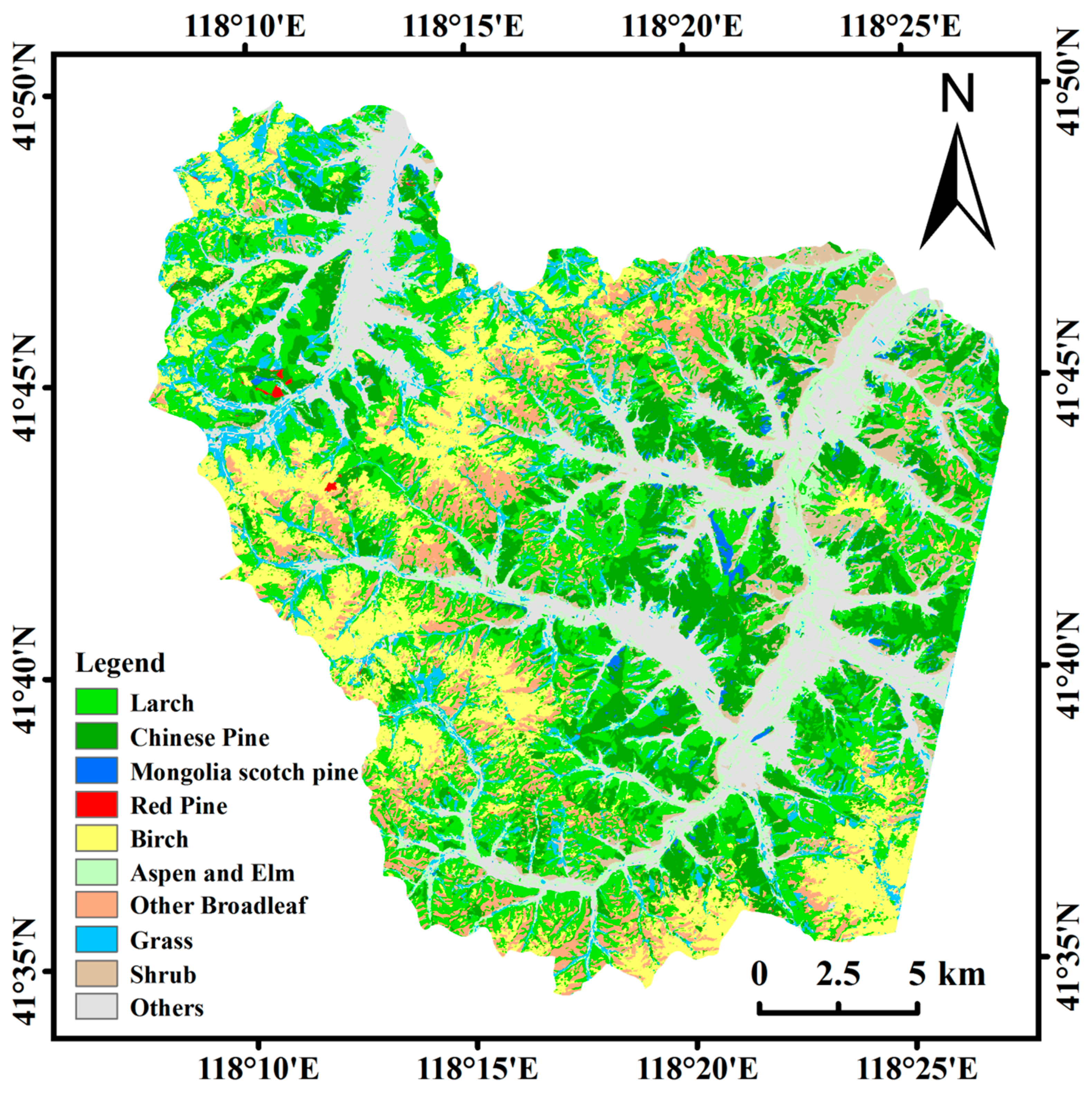
| Larch | 133.89 | 26.78 |
| Birch | 75.50 | 15.10 |
| Chinese pine | 67.22 | 13.45 |
| Aspen and elm | 36.08 | 7.22 |
| Other broadleaf tree species | 35.04 | 7.01 |
| Mongolia scotch pine | 3.60 | 0.72 |
| Red pine | 0.55 | 0.11 |
| Grass | 33.21 | 6.64 |
| Shrub | 32.78 | 6.56 |
| Farmland | 58.30 | 11.66 |
| Impervious surface area | 12.74 | 2.55 |
| Bare land | 10.48 | 2.10 |
| Water | 0.48 | 0.10 |
| Data Scenarios | Overall Forest Classification Accuracies (%) Based on Six Algorithms | ||||||
|---|---|---|---|---|---|---|---|
| MLC | ANN | kNN | DT | RF | SVM | ||
| Data from leaf-off season | V1off | 80.96 | 34.79 | 62.26 | 61.06 | 69.65 | 67.41 |
| V2off | 84.09 | 44.77 | 81.48 | 73.67 | 71.47 | 82.33 | |
| V3off | 82.85 | 55.90 | 65.99 | 73.92 | 72.91 | 81.78 | |
| Data from leaf-on season | V1on | 76.43 | 54.44 | 63.02 | 67.81 | 70.13 | 59.05 |
| V2on | 82.42 | 62.32 | 71.90 | 74.88 | 73.51 | 82.87 | |
| V3on | 83.61 | 54.98 | 76.66 | 75.48 | 83.01 | 84.76 | |
| Combined data from both seasons | V1both | 88.20 | 71.19 | 71.44 | 71.75 | 76.08 | 76.07 |
| V2both | 89.22 | 72.41 | 85.02 | 82.12 | 88.12 | 88.39 | |
| V3both | 89.41 | 68.14 | 85.85 | 82.15 | 88.78 | 88.16 | |
| Category | Dataset | Approach | Accuracy Based on Seasonal Data | Difference Between | |||
|---|---|---|---|---|---|---|---|
| Different Seasons | Comb. of Both Seasons | Comb.& Leaf-Off | Comb.& Leaf-On | ||||
| leaf-off | leaf-on | ||||||
| All land cover types | V1 | Maximum likelihood | 68.62 | 66.72 | 76.39 | 7.77 | 9.67 |
| Machine learning | 57.92 | 63.20 | 72.87 | 14.95 | 9.67 | ||
| V2 | Maximum likelihood | 76.10 | 72.14 | 80.06 | 3.96 | 7.92 | |
| Machine learning | 73.46 | 78.59 | 84.46 | 11.00 | 5.87 | ||
| V3 | Maximum likelihood | 76.10 | 73.02 | 78.59 | 2.49 | 5.57 | |
| Machine learning | 74.49 | 78.89 | 83.14 | 8.65 | 4.25 | ||
| All forest types | V1 | Maximum likelihood | 80.96 | 76.43 | 88.20 | 7.24 | 11.77 |
| Machine learning | 69.65 | 70.13 | 76.08 | 6.43 | 5.95 | ||
| V2 | Maximum likelihood | 84.09 | 82.42 | 89.22 | 5.13 | 6.80 | |
| Machine learning | 82.33 | 82.87 | 88.39 | 6.06 | 5.52 | ||
| V3 | Maximum likelihood | 82.85 | 83.61 | 89.41 | 6.56 | 5.80 | |
| Machine learning | 81.78 | 84.76 | 88.78 | 7.00 | 4.02 | ||
| All land cover types | v2&v1 | Maximum likelihood | 7.48 | 5.42 | 3.67 | ||
| Machine learning | 15.54 | 15.39 | 11.59 | ||||
| v3&v2 | Maximum likelihood | 0.00 | 0.88 | −1.47 | |||
| Machine learning | 1.03 | 0.30 | −1.32 | ||||
| All forest types | v2&v1 | Maximum likelihood | 3.13 | 5.99 | 1.02 | ||
| Machine learning | 12.68 | 12.74 | 12.31 | ||||
| v3&v2 | Maximum likelihood | −1.24 | 1.19 | 0.19 | |||
| Machine learning | −0.55 | 1.89 | 0.39 | ||||
| Tree Species Type | Data from Leaf-Off Season | Data from Leaf-On Season | Combined Both Seasons | ||||||
|---|---|---|---|---|---|---|---|---|---|
| Data | Classifier | TSMA (%) | Data | Classifier | TSMA (%) | Data | Classifier | TSMA (%) | |
| Larch | V1 | MLC | 80.1 | V1 | MLC | 77.2 | V1 | MLC | 83.6 |
| V2 | SVM/kNN | 79.9/79.3 | V2 | SVM/MLC | 72.7/71.8 | V2 | SVM | 87.3 | |
| V3 | SVM | 77.7 | V3 | RF/SVM | 73.6/73.0 | V3 | SVM/RF | 86.7/86.3 | |
| Chinese pine | V1 | kNN | 89.2 | V1 | DT/MLC | 79.2/78.8 | V1 | MLC | 92.5 |
| V2 | MLC/SVM | 89.2/88.1 | V2 | MLC | 83.6 | V2 | RF/MLC | 91.6/91.4 | |
| V3 | MLC | 91.4 | V3 | MLC | 82.9 | V3 | RF/MLC | 92.2/91.4 | |
| Mongolia scotch pine | V1 | MLC | 87.9 | V1 | kNN/MLC | 80.1/79.6 | V1 | MLC | 96.8 |
| V2 | SVM/MLC | 88.9/88.6 | V2 | MLC | 81.1 | V2 | MLC/kNN | 93.6/92.5 | |
| V3 | MLC | 90.1 | V3 | RF | 91.2 | V3 | kNN/MLC | 93.8/93.6 | |
| Red pine | V1 | MLC/kNN | 96.7/96.7 | V1 | RF/kNN | 98.3/98.3 | V1 | MLC/RF | 96.7/96.7 |
| V2 | MLC | 98.3 | V2 | SVM/MLC | 98.4/98.3 | V2 | DT/MLC | 98.4/96.7 | |
| V3 | MLC | 98.3 | V3 | SVM/MLC | 98.4/98.3 | V3 | DT | 100 | |
| Birch | V1 | MLC | 68.2 | V1 | MLC | 57.9 | V1 | MLC | 78.5 |
| V2 | SVM | 79.1 | V2 | MLC/SVM | 79.7/79.0 | V2 | SVM/MLC | 84.1/82.5 | |
| V3 | SVM | 84.5 | V3 | MLC/SVM | 81.7/80.8 | V3 | SVM/MLC | 84.1/82.5 | |
| Aspen and elm | V1 | MLC | 65.3 | V1 | MLC | 58.5 | V1 | MLC | 74.4 |
| V2 | kNN/MLC | 83.0/80.1 | V2 | SVM | 84.4 | V2 | SVM | 92.9 | |
| V3 | SVM | 80.8 | V3 | SVM | 85 | V3 | SVM | 94.3 | |
| Other broadleaf trees | V1 | MLC | 82.1 | V1 | RF/ANN | 90.4/90.1 | V1 | MLC/RF | 95.1/93.3 |
| V2 | kNN | 91.1 | V2 | SVM | 94.2 | V2 | MLC/SVM | 95.2/95.2 | |
| V3 | MLC | 74.1 | V3 | DT/RF | 93.5/92.3 | V3 | MLC/RF | 96.2/96.2 | |
© 2019 by the authors. Licensee MDPI, Basel, Switzerland. This article is an open access article distributed under the terms and conditions of the Creative Commons Attribution (CC BY) license (http://creativecommons.org/licenses/by/4.0/).
Share and Cite
Xie, Z.; Chen, Y.; Lu, D.; Li, G.; Chen, E. Classification of Land Cover, Forest, and Tree Species Classes with ZiYuan-3 Multispectral and Stereo Data. Remote Sens. 2019, 11, 164. https://doi.org/10.3390/rs11020164
Xie Z, Chen Y, Lu D, Li G, Chen E. Classification of Land Cover, Forest, and Tree Species Classes with ZiYuan-3 Multispectral and Stereo Data. Remote Sensing. 2019; 11(2):164. https://doi.org/10.3390/rs11020164
Chicago/Turabian StyleXie, Zhuli, Yaoliang Chen, Dengsheng Lu, Guiying Li, and Erxue Chen. 2019. "Classification of Land Cover, Forest, and Tree Species Classes with ZiYuan-3 Multispectral and Stereo Data" Remote Sensing 11, no. 2: 164. https://doi.org/10.3390/rs11020164
APA StyleXie, Z., Chen, Y., Lu, D., Li, G., & Chen, E. (2019). Classification of Land Cover, Forest, and Tree Species Classes with ZiYuan-3 Multispectral and Stereo Data. Remote Sensing, 11(2), 164. https://doi.org/10.3390/rs11020164