Enhanced Measurements of Leaf Area Density with T-LiDAR: Evaluating and Calibrating the Effects of Vegetation Heterogeneity and Scanner Properties

Abstract

Reliable measurements of the 3D distribution of Leaf Area Density (LAD) in forest canopy are crucial for describing and modelling microclimatic and eco-physiological processes involved in forest ecosystems functioning. To overcome the obvious limitations of direct measurements, several indirect methods have been developed, including methods based on Terrestrial LiDAR scanning (TLS). This work focused on various LAD estimators used in voxel-based approaches. LAD estimates were compared to reference measurements at branch scale in laboratory, which offered the opportunity to investigate in controlled conditions the sensitivity of estimations to various factors such as voxel size, distance to scanner, leaf morphology (species), type of scanner and type of estimator. We found that all approaches to retrieve LAD estimates were highly sensitive to voxel size whatever the species or scanner and to distance to the FARO scanner. We provided evidence that these biases were caused by vegetation heterogeneity and variations in the effective footprint of the scanner. We were able to identify calibration functions that could be readily applied when vegetation and scanner are similar to those of the present study. For different vegetation and scanner, we recommend replicating our method, which can be applied at reasonable cost. While acknowledging that the test conditions in the laboratory were very different from those of the measurements taken in the forest (especially in terms of occlusion), this study revealed existence of strong biases, including spatial biases. Because the distance between scanner and vegetation varies in field scanning, these biases should occur in a similar manner in the field and should be accounted for in voxel-based methods but also in gap-fraction methods.

1. Introduction

Capturing the three-dimensional (3D) structure and the spatial heterogeneity of vegetation canopies is crucial for characterizing ecosystems mass and energy fluxes. 3D leaf distribution has become a critical parameter for modelling radiative transfers [1] and for eco-physiological models incorporating photosynthesis and transpiration processes [2,3]. Moreover, the vegetative element distribution is an important characteristic of forest stand conditions, which affects carbon cycling, wildlife habitat [4], or disturbances and stresses such as wildfire [5]. It is hence a key parameter to monitor.

Foliage density or Leaf Area Density (LAD, m²/m³), defined as the one-sided area of leaves per unit volume [6], can theoretically be retrieved from direct measurement of the surface area of leafy elements in reference volumes of interest. However, such an approach is not practical and remains volume limited, as it is extremely time consuming and has obvious destructive consequences on vegetation. As a result, foliage area density is often quantified through a vertical integration, namely the Leaf Area Index (LAI), which can be indirectly measured using ground-based methods [6,7,8]. However, these methods do not provide the 3D foliage distribution and require empirical corrections to account for clumping [9].

With a dense and regular laser sampling, Terrestrial LiDAR (Light Detection and Ranging) scanning, hereafter referred to as TLS, has a great potential to characterize vegetation 3D structure. TLS technology relies on a high frequency emission/reception of low divergent laser beams with registration of the 3D coordinates associated to each laser hit. As a result, TLS acquires dense 3D point clouds, providing a high-resolution representation of forest canopies. Several attempts to retrieve foliage attributes from TLS have led to encouraging results, based either on the measurement of gap fractions [10,11] or on the estimation of LAD in voxels [12,13,14,15]. Gap fraction approaches generally assume homogeneous layers to estimate effective LAD profile and use a factor to correct for clumping effect [11,15]. In contrast to gap fraction approaches, the voxel-based methods, which are studied in the present paper, explicitly account for vegetation heterogeneity (i.e., clumping effect) at scales larger than voxel size.

These voxel methods use various metrics to estimate the LAD, based on different estimators of the attenuation coefficient, which is the rate at which vegetation attenuates beam transmission. The Relative Density Index (RDI) is the ratio of number of hits inside a voxel to the number of beams entering the voxel [16] and is an empirical measurement of vegetation absorbance [15]. Voxel-based methods rely on different functional forms of the RDI or other statistics such as the mean path length (mean distance potentially explored by beams within a voxel assuming no element intercepted them) and the mean free path length (mean distance actually explored by beams within a voxel) [15]. These indices can be readily applied or combined with field measurements through a calibration phase [14]. The voxel-based canopy profiling method [17] was developed for very small voxel sizes (below 10 cm) and uses ratios of full versus empty voxels to compute RDI. For larger voxel sizes, intra-voxel LAD estimators can be computed, using the relative density index [14,16], the contact frequency [18], the modified contact frequency [12] and the Beer-Lambert law [13,19,20]. Intra-voxel estimators were recently compared using a theoretical framework and numerical experiments [15].

A key characteristic of vegetation when retrieving LAD in these formulations is the leaf orientation. Indeed, the estimated attenuation coefficient is the projected leaf area density of the voxel in the plane perpendicular to the direction of emission of the laser beam. This projection ratio depends on leaf orientation and is accounted for with the G factor [12]. The value attributed to G for random leaf orientation is 0.5 (i.e., the projected area is half the one-sided leaf area). Determining the exact G value in voxels with TLS is challenging [13] but is now possible for large leaves [20]. Regarding small elements, no method has gained a consensus yet but it has been shown that branches (and by extension leaves) orientation has a limited impact on the quality of results, even for planophile and erectophile distributions [13,14,21], supporting the validity of an assumption of G = 0.5. Another critical aspect is the differentiation between leaf and wood return, as the final objective of these methods is to determine the LAD and not the PAD (Plant Area Density, which includes both leaf and wood surface areas).

The theoretical bases supporting these methods generally assume that vegetation elements are small and randomly distributed within a voxel [12,15]. As leaf clumps are surrounded by empty volumes, voxels should be small enough to discretize large gaps between branches [22]. Indeed, aggregating empty spaces and leaf clumps in a single large voxel leads to a systematic underestimation of predicted leaf area, as a consequence of Jensen’s inequality [23,24], as suggested in Reference [15]. However, smaller voxels do not necessarily increase the accuracy of the estimation. Indeed, the voxels should be large enough with respect to the size of vegetation elements, otherwise leading to an overestimation of the LAD [22]. Also, smaller voxels cause a sharp rise in the variability of LAD estimates, as it decreases the number of beams and the number of vegetation elements in voxels [15]. It should be noted, however, that theoretical corrections can be implemented to account for element size and number of beams [15].

In addition to biases inherent to vegetation structure, the instrument can introduce deviations from actual LAD values, mostly as a consequence of the finite cross-sectional diameter of the scanner beam, in particular with single return phase shift scanners. A laser beam can indeed partly hit a leaf, while a remaining—not intercepted—fraction of laser energy continues its path before possibly interacting with another object located in the background. In this case, a single return phase-shift scanner registers a unique point which can be anywhere between the two objects, leading to a hit misplacement (mixed points, [25]). As a result, different backgrounds (vegetated vs. 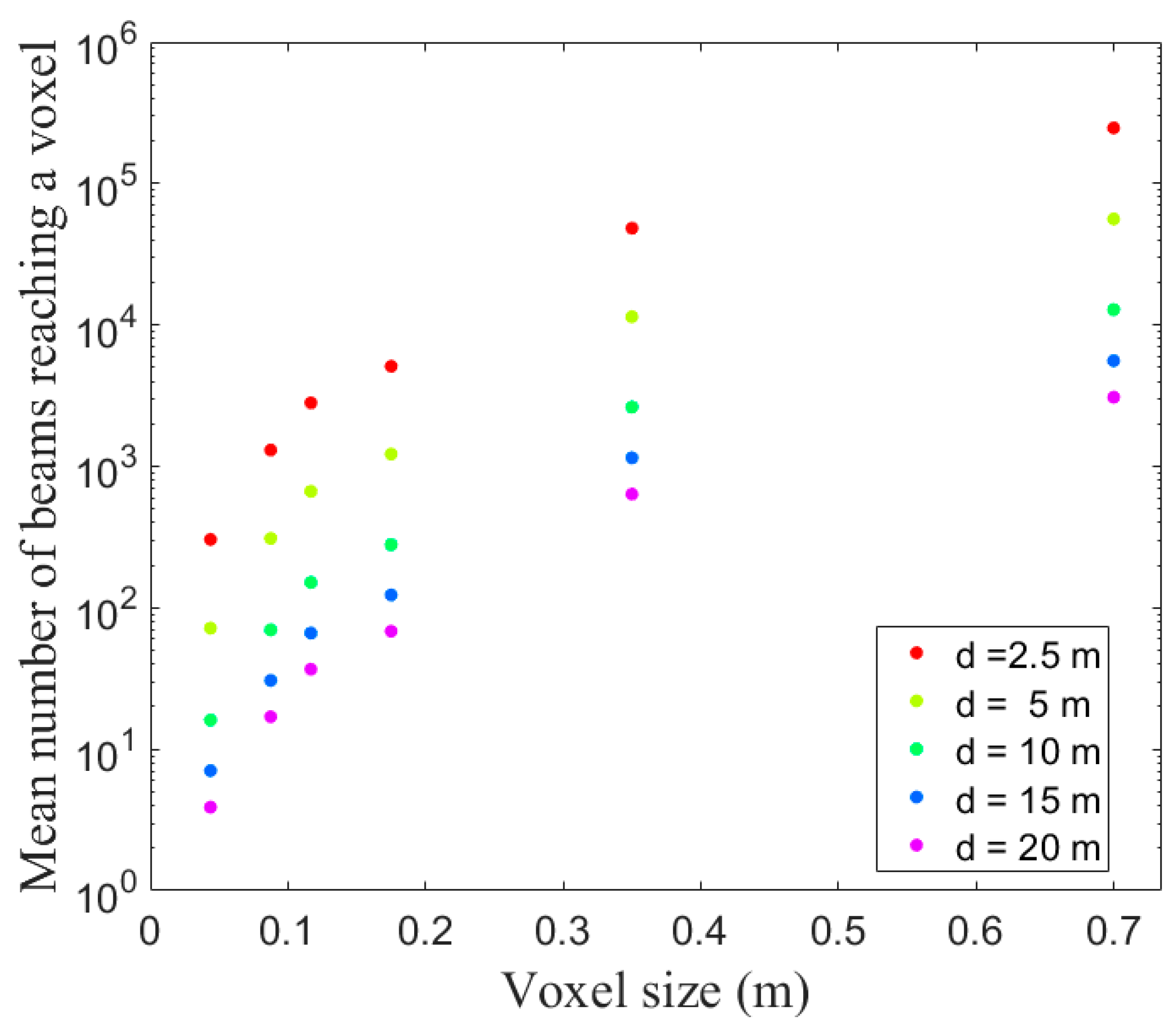open) may affect any partial hit of vegetation elements and in turn, LAD predictions. In addition, as the footprint (cross-sectional area) of a laser beam increases with distance to scanner (because of beam divergence), the probability to hit vegetation elements increases, which induces an increase in the LAD estimation with distance to scanner. Such bias can be corrected by weighting estimated RDI, with distance-dependent calibrated function of return intensity [12] but to date, this approach was only applied at fixed distance only (scanning individual plants at constant distance to the scanner). Finally, the limited number of beams effectively reaching a voxel is a last source of bias and uncertainty in TLS measurement [15]. Low beam number arises from both increasing distance to scanner and vegetation occlusion.

Hence, the three sources of bias –theoretical, vegetation and instrument- of LAD estimates are sensitive to both voxel size and distance to scanner. Indeed, variations in voxel size affect the number of beams, the relative size of vegetation element (compared to voxel size) and the discretization of vegetation structure (i.e., how clumps and gaps are discretized). Also, increased distance to scanner decreases the number of beams, increases the probability of hit and decreases returned energy (so detection ability). Among the different sources of bias, some of them can be theoretically corrected, as suggested in Reference [15].

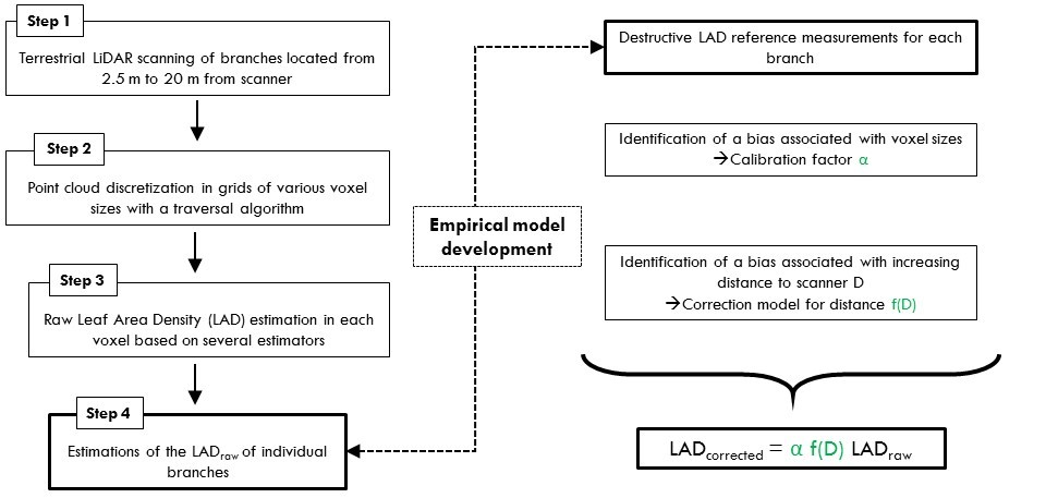
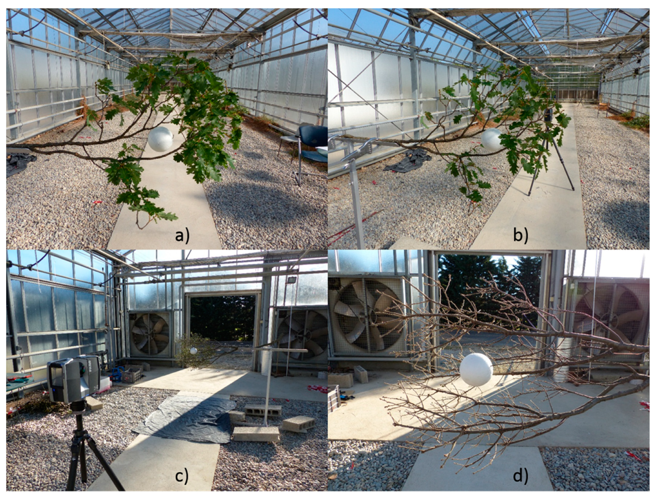
This study aims to (i) disentangle the different sources of bias and to evaluate their magnitude, (ii) focus on the specific biases associated with voxel size and distance to scanner and (ii) propose generic calibration models to retrieve correct LAD estimates from TLS measurements. To achieve these objectives, we worked on tree branches in a controlled environment with negligible occlusion. Accurate destructive LAD reference values were available for 46 branches. We first investigated the performances of five different voxel-based methods for estimating the LAD of vegetation samples. In particular, these estimators were tested on three species with distinct foliage shapes, sizes and clumping patterns. Secondly, we investigated the sensitivity of the predictions to discretization (voxel-size effect) and distance to scanner (distance effect). These analyses were carried out with two scanners (one phase shift and one time of flight scanner), which expands the scope of our results.

2. Materials and Methods

2.1. Vegetation Sampling and Set-Up

Three Mediterranean tree species, Quercus pubescens, Quercus ilex and Pinus halepensis, with different foliar morphologies were sampled. For each species, a set of branches were collected in the Luberon regional Natural Park, in South-eastern France. Q. pubescens branches were collected in pure stands located near Lioux (5°20′55.5497″E–44°0′16.6309″N, 750 m elevation) on medium-sized trees, up to 10 m height. This species is deciduous with lobed leaves, usually 4–8 cm long and 3–5 cm wide, mostly located at the end of the twigs. Q. ilex and P. halepensis branches were collected in mixed stands (that include both species) located near Cheval-Blanc (5°7′25.1998″E–43°47′14.1000″N, 350 m elevation). Q. ilex is an evergreen species with dense and leafy branches. Trees used for collection of branches were smaller than 6 m height. Leaves are narrowly oval, most often 3–5 cm long and 1.5–2 cm wide. P. halepensis is a medium-sized conifer, up to 12 m at the study site. Its thin needles, about 1–2 mm wide and 6–10 cm long, are grouped in dense shoots. Needles and leaves are later referred to as vegetation elements.

We sampled 10 branches for Q. pubescens, 20 for Q. ilex and 16 for P. halepensis (

Table 1. Characteristics of branch samples for the three species and three foliage conditions.

Species	Scanner	Number of Branches 1	$\overline{\mathit{S}\mathit{L}\mathit{A}}$(m2·kg−1)	$\mathit{Projected} \mathit{Area} \overline{{\mathit{A}}_1}$(cm2)	Foliage Condition	$\overline{\mathit{L}\mathit{A}{\mathit{D}}_{\mathit{r}\mathit{e}\mathit{f}}} ({\mathbf{m}}^2/{\mathbf{m}}^3)$	Leaf Fraction $\overline{\mathit{L}}$
P. halepensis	FARO, RIEGL	10 Veg. B. (FARO)+ 6 Open B. (FARO/RIEGL)	3.12 +/− 0.15	0.43 +/− 0.08	Leaf on	3.14 +/− 1.55	0.77 +/− 0.12
					Half defoliated	1.43 +/− 0.65	0.52 +/− 0.14
					Leaf off	0	0
Q. ilex	FARO, RIEGL	14 Veg. B. (FARO)+ 6 Open B. (FARO/RIEGL)	6.08 +/− 0.64	4.03 +/− 1.53	Leaf on	3.09 +/− 0.99	0.85 +/− 0.04
					Half defoliated	1.43 +/− 0.45	0.7 +/− 0.07
					Leaf off	0	0
Q. pubescens	FARO	10 Veg. B. (FARO)	11.65 +/− 2.80	17.0 +/− 3.6	Leaf on	2.45 +/− 0.75	0.89+/− 0.06
					Half defoliated	1.21 +/− 0.39	0.76 +/− 0.08
					Leaf off	0	0

¹ Veg. B. corresponds to “vegetated background,” whereas Open B. corresponds to “open background.”

), within a wide range of local vegetation densities, at various heights and light exposures. To avoid leaf desiccation, branches were collected at dawn and immediately brought back to the laboratory, watered and stored in a refrigerated room and were scanned within 24 h. Each collected branch was horizontally fixed to a tripod by its woody extremity. A 10-cm diameter spherical polystyrene target was fixed in the middle of the branch foliage as a reference target in the scanner point cloud (Figure 1). In order to control the spatial extent of the vegetation, branches were pruned so that all twigs and leaves located beyond 35 cm from the centre of the sphere were manually removed, using a 30-cm stick touching the sphere (5 cm radius) in all directions to decide whether vegetation elements should be pruned. The only exception was the thick woody material supporting vegetation.

In order to extend the range of both the foliar densities and ratios of element mixture (leaf/wood ratio) of scanned branches, each pruned branch was scanned under three foliage conditions. They were first scanned with all their leaves (leaf-on condition, e.g., Figure 1a,c). Then, approximately half of the initial number of leaves/needles was manually removed and stored separately and the branch was scanned again (half-foliated condition, e.g., Figure 1b). Finally, the remaining leaves were removed and stored, then a final scan was performed (leaf-off condition, e.g., Figure 1d).

The measurements were carried out at two different locations: in a greenhouse at INRA in Avignon and in a facility at IRSTEA in Montpellier. This choice was dictated by the usage of the RIEGL scanner, which was not owned by our research team. Both experimental locations were well-sheltered from wind and experimental conditions were similar. Yet, one noticeable difference between the two experimental sites was the background when the branches were scanned. This background was vegetated at short distance (at about 15 m) at the INRA site (see Figure 1), later referred to as “Veg. Back.,” whereas the outside of the IRSTEA facility was characterized by an obstacle-free distance of at least 100 m in the scan direction. This background was later referred to as “Open Back.”. As stated in the introduction, these differences in backgrounds are likely to affect the distribution of mixed pixels and thus the LAD predictions.

2.2. Vegetation Reference Measurements

For each collected branch, we determined the reference leaf area density ${LAD}_{ref}$ (in m²/m³ or equivalently, in m⁻¹), defined as the half total area of leaves per unit volume, for both half-defoliated and leaf-on conditions. For that purpose, leaf samples were collected just after the branch was scanned and were oven-dried and weighed to determine the dry mass of leaves/needles (${\mathrm{M}}_{ref}$, in kg). $LA{D}_{ref}$ was derived as follows:

$$LA{D}_{ref}=\{\begin{array}{ll}\frac{M_{ref}SLA}{V},& \mathrm{for} Q. ilex \mathrm{and} pubescens\\ \frac{\pi }{2}\frac{M_{ref}SLA}{V},& \mathrm{for} P. halepensis\end{array}$$

(1)

with $M_{ref}$ the dry mass of leaves/needles, $SLA$ the Specific Leaf Area (in m²·kg⁻¹) and $V$ the volume of vegetation of interest, that is, the virtual 0.35-m-radius sphere containing vegetation. In Equation (1), the $\frac{\pi }{2}$ factor for P. halepensis needles arises from the definition of the $SLA$, usually defined as the projected Specific Leaf Area (see Appendix A for details). The (projected) $SLA$ was estimated for each branch, by sampling $n_s$ leaves/needles within the pruned elements, with $n_s$ equal to 15, 30 and 50 for Q. pubescens, Q. ilex and P. halepensis, respectively. Each group of leaves/needles was scanned with a standard A4 flatbed Epson scanner at 600 dpi. Vegetation pixels were identified in scanned images with GRASS software (GRASS Development Team, 2017) based on a colour threshold (green channel) and the projected leaf area of the sample ($A_s$, in m²) was retrieved by summing these pixels. Vegetation elements were oven-dried at 60 °C and weighed ($M_s$, in kg). The (projected) SLA was computed as:

$$SLA=\frac{A_s}{M_s}$$

(2)

The mean and range of $LA{D}_{ref}$ are reported in Table 1. The reference volume used for density computation was the 0.35-m-radius sphere in which vegetation was located.

We also estimated ${\lambda }_1$, the attenuation coefficient associated with a single vegetation element, which is used to correct LAD estimates when element size is large, compared to voxel size ([15], see

Table 2. Formulation and characteristics of the attenuation coefficient estimators (see [15] for details).

Symbol	Name	Bias Correction			Formulation
		Unequal Path Length	Element Size	Beam Number
$\mathrm{CF}$	Contact frequency [18]	No	No	No	$\frac{\mathrm{RDI}}{\overline{\delta }}$
$\tilde{\lambda }$	Modified Contact frequency [12]	Not required	No	No	$\frac{\mathrm{RDI}}{\overline{z}}$
$\tilde{\mathsf{\Lambda }}$	Theoretical Bias-corrected (TBC) MLE [15]	Not required	Yes 4	Yes 5	$\frac{\mathrm{RDI}}{\overline{z_e}}-\frac{\overline{1_{z<\delta }{z}_e}}{N{\overline{z_e}}^2}$
$\hat{\lambda }$	Beer-Lambert [19]	No	No	No	$-\frac{\log \left(1-\mathrm{RDI}\right)}{\overline{\delta }}$
${\hat{\mathsf{\Lambda }}}_2$	Theoretical Bias-corrected (TBC) Beer-Lambert [15]	Yes 1	Yes 2	Yes 3	${\hat{\mathsf{\Lambda }}}_2=\frac{1}{a_e}\left(1-\sqrt{1-2a_e\hat{\mathsf{\Lambda }}}\right)$ with $\hat{\mathsf{\Lambda }}=\{\begin{array}{c}-\frac{1}{\overline{{\delta }_{\mathrm{e}}}}\left(\log \left(1-\mathrm{RDI}\right)+\frac{\mathrm{RDI}}{2N\left(1-\mathrm{RDI}\right)}\right) \mathrm{when} \mathrm{RDI}<1\\ \frac{\log \left(2N+2\right)}{\overline{{\delta }_e}} \mathrm{when} \mathrm{RDI}=1\end{array}$

¹${\hat{\mathsf{\Lambda }}}_2$ is a square root function of $\widehat{\mathsf{\Lambda }}$ to account for unequal path length. ² The mean path length $\overline{\delta }$ is replaced by the “effective” mean path length $\overline{{\delta }_e}=mean\left(-\frac{log\left(1-{\lambda }_1{\delta }_j\right)}{{\lambda }_1}\right)$. ³ With the term in 1/N, with N the beam number. ⁴ The mean free path $\overline{z}$ is replaced by the “effective” mean free path $\overline{z_e}=mean\left(-\frac{log\left(1-{\lambda }_1{z}_j\right)}{{\lambda }_1}\right)$. ⁵ With the term in 1/N, with N the beam number.

for the formulation of the correction). It is defined as the ratio between the element cross-sectional area $S_1$ (m²) and the volume $v$ (m³) of the voxels used for the voxelization of TLS data (see Section 2.5). ${\lambda }_1$ is computed as a function of the projected area of a single element $A_1=\frac{A_s}{n_s}$ (see Appendix A for details):

$${\lambda }_1= \frac{S_1}{v} \mathrm{with} S_1=\{\begin{array}{ll}\frac{A_1}{2},& \mathrm{for} Q. ilex \mathrm{and} pubescens\\ \frac{\pi A_1}{4},& \mathrm{for} P. halepensis\end{array}$$

(3)

The mean and range of $A_1$ are reported in Table 1.

Finally, we determined the leaf fraction $L$, defined as the leaf contribution to the attenuation coefficient in a vegetation sample. Indeed, vegetation samples were mixtures of twigs and leaves/needles, hence the attenuation coefficient of the mixture ${\lambda }_m$ depends on the areas of both components. Let ${\lambda }_l$ be the attenuation coefficients for respectively “leaf only” or “half defoliated” and ${\lambda }_w$ be the attenuation coefficient corresponding to “leaf off” conditions. Assuming that leaves and twigs were randomly distributed, the leaf fraction is:

$$L=\frac{{\lambda }_l}{{\lambda }_m}=\frac{{\lambda }_m-{\lambda }_w}{{\lambda }_m}$$

(4)

In Equation (4), we used the theoretical bias-corrected (TBC) Maximum Likelihood Estimation (MLE) approach (see next subsection and Table 2) to estimate ${\lambda }_m$ (leaf on or half defoliated, depending on the corresponding sample) and ${\lambda }_w$ (leaf off) from TLS point clouds at short distance (i.e., 2.5 m). Indeed, MLE estimator is theoretically unbiased and is supposed to exhibit the lowest residual variance. In addition, estimates are expected to be the most accurate at short distance, where the number of beams is the highest and the beam divergence is the smallest.

Means and standard deviations of leaf fractions are presented in Table 1.

2.3. TLS Scanners and Scan Design

Two scanners instruments were used in this study: the FARO Focus3D X 130 (FARO Technologies Inc., Lake Mary, FL, USA) and the RIEGL VZ-400 (RIEGL Laser Measurements Systems GmbH, Horn, Austria). The FARO instrument is a phase-shift laser scanner (Amplitude Modulated Continuous Wave) operating at 1550 nm wavelength. Its maximal angular resolution is 0.009°. Laser beams are emitted with a diameter of 2.25 mm at exit and diverge by 0.19 mrad (diameter increases by 19 mm per 100 m). The RIEGL scanner is a time-of-flight scanner (short laser pulses are emitted and distance measurements are based on elapsed time between the emission of a pulse and the reception of the backscattered signal) using near infrared wavelength. Its angular resolution can be set between 0.0024° and 0.288°. Laser beams are emitted with a diameter of 6.5 mm at exit with a divergence of 0.35 mrad. Measurement errors are 0.3 mm at 25 m and 5 mm at 100 m for the FARO and the RIEGL scanners, respectively. The RIEGL VZ-400 is a multi-echo scanner. However, multiple echoes cannot be registered at distances shorter than 80 cm, so that the RIEGL was expected to behave as a single echo scanner in our experiment, since vegetation elements were located in a 70 cm diameter sphere.

In this study, the FARO and RIEGL scanners were both set to a resolution of 0.036°, a good compromise to collect dense point clouds while successfully addressing practical issues such as operational time and data storage management during field campaigns. The acquisitions with the FARO system were performed without “clear contour” and “clear sky” FARO filters, which respectively remove mixed pixels and sky returns [14,26], as all beams should be tracked by the traversal algorithm, in order not to bias the estimated quantities. Such filters are not available when acquiring data with the RIEGL system.

To evaluate the influence of the distance to the scanner on LAD estimations, scans were performed at five distances from the vegetation sample (d = 2.5 m, 5 m, 10 m, 15 m and 20 m) for each foliage condition (leaf on, half defoliated, leaf off), hence providing a total of 15 scans per branch. Among other effects, the number of beams reaching a voxel decreases with the distance to the scanner (Figure 2). As shown in Figure 2, from 2.5 to 20 m, this number is roughly divided by 100.

2.4. Processing TLS Point Clouds

2.4.1. Pre-Processing

This step consisted in (i) registering raw scans, (ii) determining the coordinates of the polystyrene sphere (centre of the sample) and (iii) exporting point clouds in a format adapted to retrieving beam trajectory even when no return was registered. This last point is crucial for the computation of Relative Density Index (RDI) with a traversal algorithm (see below), as beams with no return should not be ignored but counted as beams with no interception with vegetation.

We used SCENE 5.3 (FARO Technologies Inc.) and RiSCAN PRO software for FARO and RIEGL scans, respectively, to retrieve the coordinates of the polystyrene spheres and to export point clouds in the gridded. ”ptx” format, which enables trajectory retrieving when no returns were registered ([27]).

2.4.2. Traversal Ray-Tracing Algorithm

We used a traversal algorithm developed in Matlab software (The MathWorks, Inc., Natick, MA, USA) that computes the intersections of each individual beam (defined as the line passing through scan centre and return position) and a given computational grid. Here, the computational grid was a 3D regular grid centred on the spherical target. Grid spacing was referred to as “voxel size” and sets the level of discretization of the vegetation. Tested voxel sizes were 0.04 m, 0.09 m, 0.12 m, 0.18 m, 0.35 m and 0.70 m. The algorithm determines if a beam was intercepted before, inside or passed through a given voxel. It thus computes, for each voxel, the number of hits and number of beams passing through, the RDI (which is the ratio of the number of hits inside a voxel to the total number of beams entering the voxel), the mean free path $\overline{z}$ (mean distance actually travelled by the beams through the voxel) and the mean path length $\overline{\delta }$ (mean distance theoretically travelled by the beams through the voxel if no hit would have occurred). These different metrics were required to compute LAD with the different attenuation coefficient estimators [15], which relates to leaf area, briefly described in the next section.

The mean number of beams reaching a voxel was strongly affected by voxel size. It ranged between 4 and 20,000 and was in general in the order of a thousand.

2.4.3. Raw Leaf Area Density Estimates ($LA{D}_{raw}$)

Raw estimates refer to LAD estimates computed for various theoretical equations, prior to any calibration for voxel size, species and distance effects. According to the definition of the leaf fraction $L$ (Equation (4)), a raw estimation of the $LAD$ within the vegetation volume $V$ with a scanner was given by the summation of the contribution of all voxels:

$$LA{D}_{raw}=\frac{1}{V}{\displaystyle \sum }_{i}L\frac{{\lambda }_m^i}{G}v$$

(5)

with $G$ the projection function, $V$ the vegetation volume (0.35-m-radius sphere, in m³), $v$ the volume of a voxel (m³) and ${\lambda }_m^i$ the estimated attenuation coefficient in voxel i (m⁻¹). As no general method is yet available to determine the projection function of small elements, such as needle shoots and small leaves, we simply assumed that G was equal to 0.5. The potential biases arising from leaf orientation are thus not accounted for in this raw estimator. It is important to notice that the volume, by which the leaf area sum is divided in Equation (5), is the vegetation volume (V), rather than the sum of voxel volumes (${{\displaystyle \sum }}_{i}v$). The same constant was used to divide leaf area reference measurements (Equation (1)), which authorizes a direct comparison of raw values and reference measurements.

We evaluated several estimators of the attenuation coefficient ${\lambda }_m$, which were reported in literature [12,13,15,18]. These estimators are listed in Table 2 using the same notations as in Reference [15]. The different estimators are based on the RDI and on either the mean free path length $\overline{z}$ or on the mean path length $\overline{\delta }$. They are briefly described below.

The most basic estimator is derived from the Contact Frequency ($CF$) method, initially developed for actual probe (inclined point quadrat method [28]). The CF attenuation coefficient is estimated as the RDI divided by the mean path length $\overline{\delta }$. When applied to TLS data, this estimator is expected to be negatively biased, since the volume occluded by vegetation elements in the voxel remains unexplored [12]. It results in an overestimation of the sampled volume, leading to an underestimation of LAD, which was confirmed in Reference [18]. As a consequence, it has been suggested to modify this method (Modified Contact Frequency, MCF [12]). The MCF attenuation coefficient $\tilde{\lambda }$ is estimated by dividing the RDI by the mean free path length $\overline{z}$, instead of by the mean path length. The relevance of such a modification has been theoretically established by Reference [15], who demonstrated that the modified contact frequency was indeed the Maximum Likelihood Estimator (MLE) of the attenuation coefficient, provided that vegetation elements were small and randomly distributed. The authors also demonstrated that no specific correction of the MCF was required when path lengths were unequal, which is the case in cubic voxels [13,21]. When element size is small and/or beam number is low, the MCF is biased and can be corrected in the so called theoretical bias corrected “TBC MLE estimator” $\tilde{\mathsf{\Lambda }}$. It is important to note, that this TBC estimator implements corrections for theoretical biases but not those arising from vegetation distribution and instrument specifications. The TBC MLE is thus potentially biased in regard to actual TLS and field data, which is the subject of the present comparison.

A second class of estimators computed from RDI is based on the inversion of the usual transmission equation, known as the Beer-Lambert law. [22] successfully applied this theoretical function to assess plant-scale and voxel-scale estimations of LAD, respectively. To avoid infinite values when RDI = 1, we bounded $\widehat{\lambda }$ by $\frac{\log \left(2N+2\right)}{\overline{\delta }}$, with N the number of beams, as suggested in Reference [15]. As for the MCF, this estimator is biased when elements are large compared to voxel size [15,22] and when the number of beams is low (lower than 100, [15]) but also when the path length is unequal [13,15,19]. Following [15], we implemented bias corrections in the “TBC” Beer-Lambert estimator ${\hat{\mathsf{\Lambda }}}_2$, tested below. The “2” subscript expresses that the estimators account for unequal path length, as in Reference [15].

2.5. Bias Analysis and Calibration of the Raw Leaf Area Density Estimates

2.5.1. Analysis Overview

All above raw estimators (uncorrected and TBC) theoretically assume a homogenous sampling with infinitely thin scanner beams and a random distribution of vegetation elements [15]. Since these assumptions are not fully met due to vegetation structure and optical processes involved in LiDAR beam sampling, comparisons between $LA{D}_{raw}$ (from TLS) and $LA{D}_{ref}$ (from laboratory measurements) were expected to exhibit several biases. However, some of the theoretical biases in raw estimators are corrected and it was thus important to compare the different estimates. The corresponding analysis are described in Section 2.5.2.

Raw estimates were expected to be less biased at short distance, because laser beams had the smaller footprint and to exhibit the smallest variability, because the number of beams reaching voxels was the highest. However, even short-distance raw estimates (at 2.5 m from the scanner, labelled $LA{D}_{raw}^{d=2.5\mathrm{m}})$ were potentially influenced by (i) 2.5-m beam size and echo detection, (ii) discrepancies between the actual G value and 0.5, (iii) heterogeneity in vegetation element distribution, from shoot to branch scale. To identify the sources of variation in $LA{D}_{raw}^{d=2.5\mathrm{m}}$ with respect to $LA{D}_{ref}$, we first performed an analysis of covariance (Appendix C.2). For all estimators, the main significant effect was found to be the voxel size, on which the focus is made in Section 2.5.3 and which was accounted for through a calibration coefficient. Because voxel size used for field measurements are determined by scan design, type of vegetation, applications or even computational constraints, we attempted to provide correction over a wide range of sub-meter voxel size.

When increasing the distance to the scanner, the number of beams per voxel decreased, which was theoretically accounted in TBC estimators. However, other source of bias might exist such as variations in beam size and echo detection, associated with beam divergence. Another analysis of covariance (Appendix C.3) showed that the distance to scanner—at least for the FARO scanner—was the main source of variation in raw estimations, with respect to short distance measurements. The corresponding analysis is described in Section 2.5.4., where we developed a calibration for this “distance effect.”

The overall calibration resulting from these two calibration steps (voxel size + distance effect) is described in Section 2.5.5.

2.5.2. Estimator Comparison and Analysis of Bias Corrections Included in Estimators

The TBC MLE was used as the reference to compare $LA{D}_{raw}$ values computed using various attenuation coefficient estimators. This comparison aimed at better understanding the differences and similarities between Contact Frequency, Beer-Lambert and MLE-based predictions, with and without bias corrections for unequal path length and element size. In this study, the bias corrections for unequal path lengths in the TBC Beer-Lambert estimator (${\hat{\mathsf{\Lambda }}}_2$), as well as those for small numbers of beams (in both ${\hat{\mathsf{\Lambda }}}_2$ and the bias-corrected MLE estimator $\tilde{\mathsf{\Lambda }}$) were expected to have limited effects. Indeed, path lengths were close to equality as the beams were almost aligned with grid axes. Also, the number of beams was generally greater than 30, with the exception of very small voxels when the distance to the scanner exceeded 15 m (Figure 2).

${\hat{\mathsf{\Lambda }}}_2$ and $\tilde{\mathsf{\Lambda }}$ were also theoretically corrected for the statistical bias associated with element sizes, which exhibited variations among branches and species. For both the MLE $\tilde{\mathsf{\Lambda }}$ and the Beer-Lambert ${\hat{\mathsf{\Lambda }}}_2$ estimators, the bias correction for element size involved parameter ${\lambda }_1$, defined in Equation (3) through the calculation of an effective (free) path length (Table 2). The corresponding corrections were significant only when the product of ${\lambda }_1$ by the voxel size (optical depth of a single element in the voxel) was significantly smaller than one [15]. Appendix B shows the values of this product for the different elements and voxel size. This figure suggests that the corrections were significant only when voxel sizes were strictly smaller than 0.1 m for Q. pubescens and smaller than 0.05 m for Q. ilex.

2.5.3. Influence of the Voxel Size

We performed an analysis of covariance using type III sums of squares with several covariates (voxel size, species, type of scanner and background) on the $LA{D}_{raw}^{d=2.5\mathrm{m}}$, which established that the voxel-size effect was the most important source of bias at a short distance. This effect of voxel size was already reported in Reference [12]. Tree species were only found to be of secondary importance. No statistical effect of the type of scanner nor of the background was detected. Additional details regarding this statistical analysis can be found in Appendix C.2.

A linear model was used in order to quantify bias magnitude and to estimate a calibration coefficient $\alpha$ for each discretization level:

$$LA{D}_{ref}=\alpha LA{D}_{raw}^{d=2.5\mathrm{m}}$$

(6)

We used adjusted R² and root mean square errors (RMSE) to evaluate the performance of the different calibrated raw estimators.

2.5.4. Influence of the Distance to Scanner (Distance Effect)

Raw estimates were expected to vary with the distance to scanner d (m), as both beam size and detection threshold affect the computation of RDI [12,13]. Other processes can be involved such as the instrument measurement accuracy but also the number of beams entering the voxel, which decreased with distance and zenithal angle.

To confirm these hypotheses, we performed statistical analyses with an analysis of covariance of type III. We found that the distance to scanner has indeed a strong significant effect on estimations. This effect differed among the two scanners, the distance effect being much stronger with the FARO instrument than with the RIEGL scanner. To a lesser extent, the distance effect was found to vary with discretization levels. We also found minor differences between the distance effects observed with Pinus halepensis and the other studied species. No effect of the background was detected. The details regarding this statistical analysis can be found in Appendix C.3

The distance effect at a distance d (m) was quantified by the ratio of LAD raw value at 2.5 m to the LAD raw value at d. Hence, the calibration factor $f\left(d\right)$ used to correct the distance effect was defined as:

$$LA{D}_{raw}^{d=2.5\mathrm{m}}=f\left(d\right)LA{D}_{raw}^d$$

(7)

As the bias associated with distance was significant, we fitted a model to account for such deviation on the FARO instrument. Several nonlinear regressions were tested. Best results were obtained with:

$$f\left(d\right)={\beta }_1+ {\beta }_2{e}^{{\beta }_3.d}$$

(8)

Equation (8) accounted for an increase in $LA{D}_{raw}^d$ which saturated at long distance (${\beta }_3<0$).

2.5.5. Calibrated LAD

The calibrated LAD, corrected for both discretization and distance effects, was defined as:

$$LA{D}_{cal}=\alpha f\left(d\right)LA{D}_{raw}^d$$

(9)

Each calibrated model was evaluated according to the mean absolute percentage errors (MAPE) to reference measurements for the different species.

3. Results

Results are organized in four subsections, as described in Section 2.5. First, we compare the raw predictions arising from the different estimators. Second, we compare the raw LAD to the actual (reference) LAD and investigate how the relationship was affected by the voxel size, for short distance measurements (distance to scanner of 2.5 m). Third, we analyse the sensitivity of predictions to the distance to scanner. Finally, we present some calibration functions correcting for both voxel size and distance biases, as well as metrics to evaluate the performance of the corresponding models.

3.1. Comparison between Predictions of the Different $LA{D}_{raw}$ Estimates

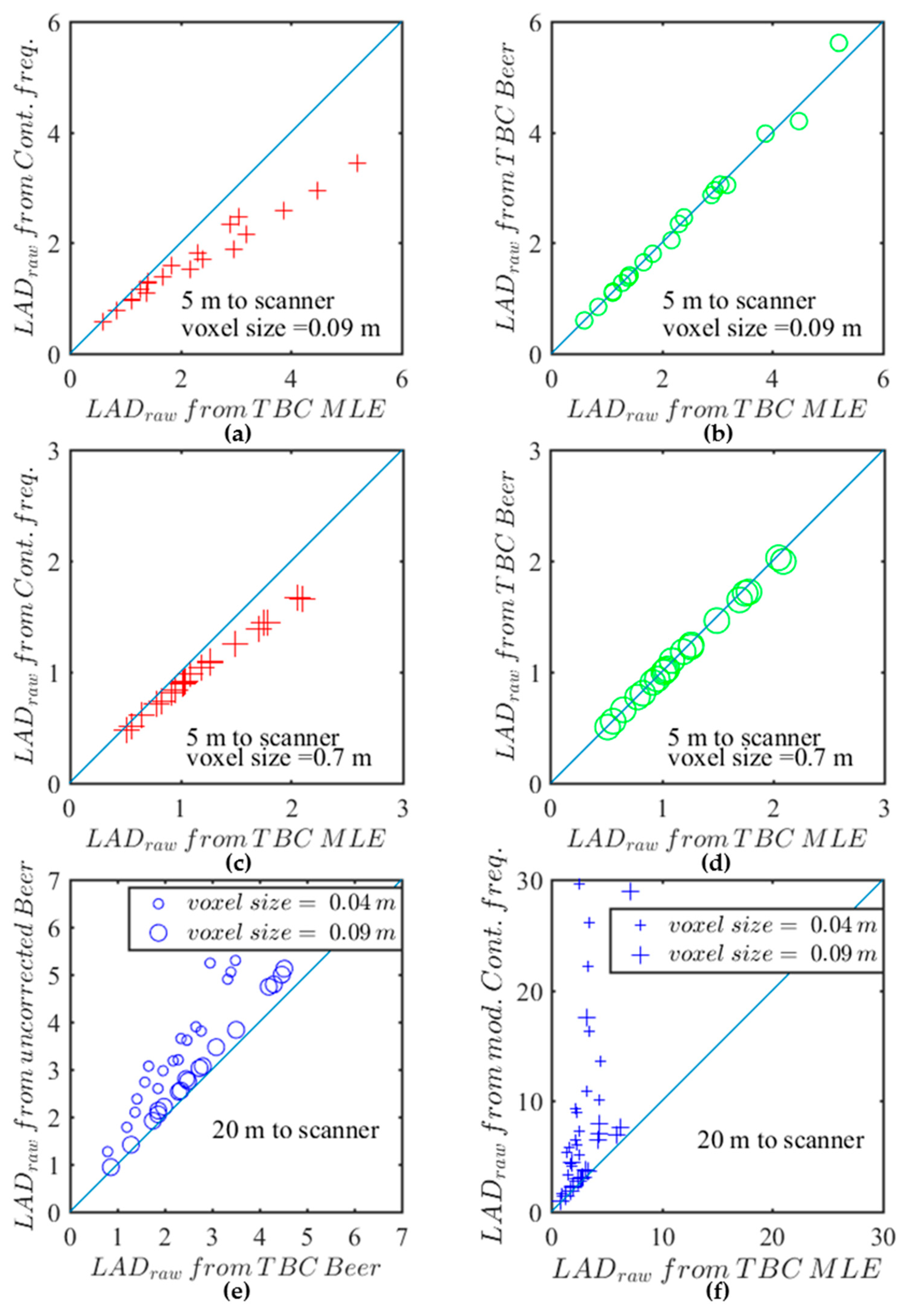
First, both TBC estimators (from Beer-Lambert law or MLE) led to very similar predictions. This is illustrated in Figure 3a,b which show both predictions for Quercus pubescens, at a distance to scanner of 5 m and for respectively Beer-Lambert law or MLE at 9 cm and 70 cm voxel sizes, revealing that they were in close agreement (green circles close to the 1:1 line). Second, Figure 3c,d show that predictions arising from the Contact Frequency were significantly lower than those from the bias-corrected MLE (red crosses). This difference can be explained by the systematic underestimation arising from the Contact Frequency method that was previously mentioned. 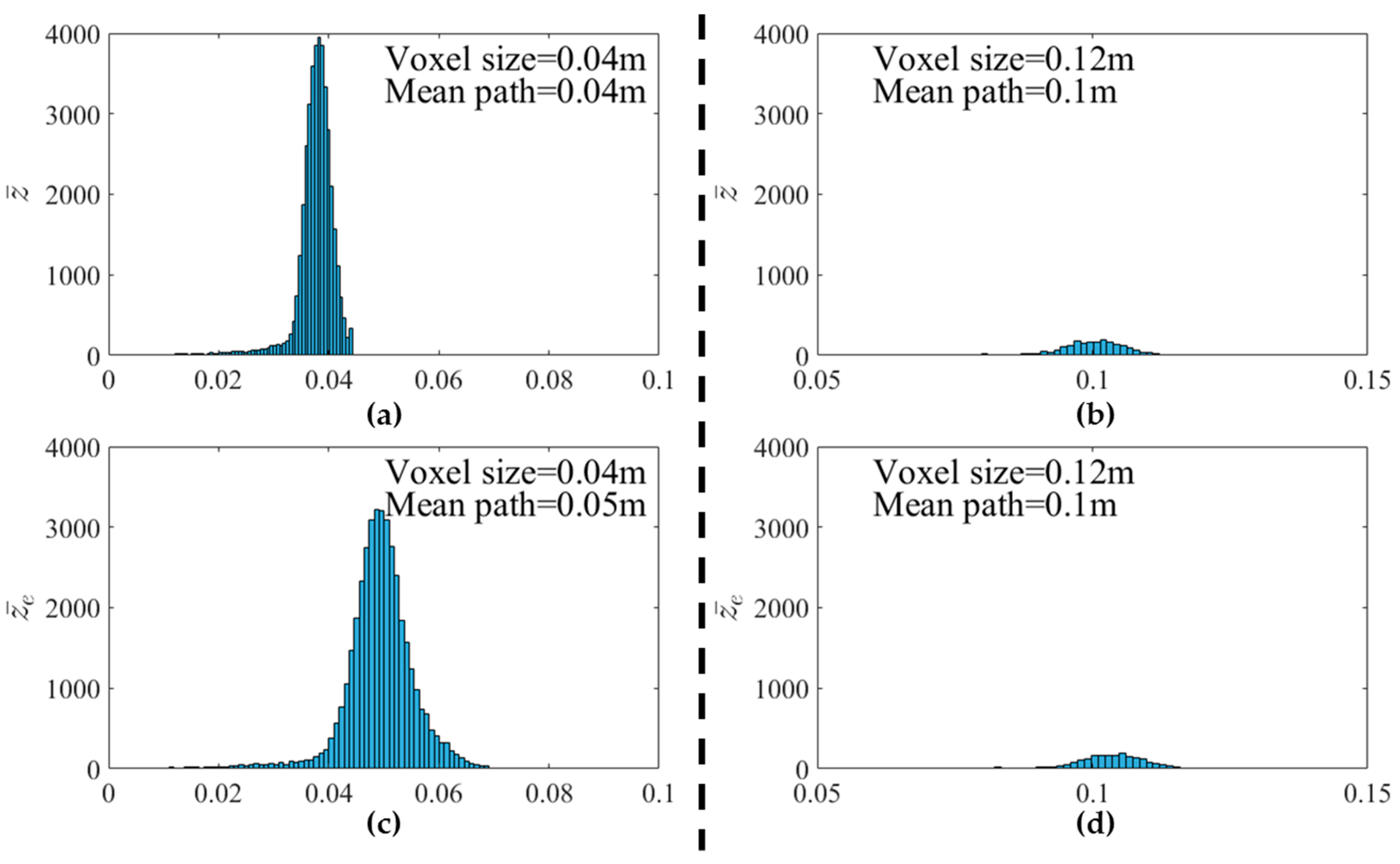Third, we found that there may be significant differences between predictions arising from TBC and corresponding uncorrected estimators when the vegetation is far from the scanner (Figure 3e,f). TBC estimators were systematically lower, especially for small voxel sizes. For example, the $LA{D}_{raw}$ computed with the TBC Beer-Lambert law were roughly 40% lower than the $LA{D}_{raw}$ computed with the uncorrected Beer-Lambert law for a 4 cm voxel size, whereas the estimates based on the TBC MLE were up to 100% lower than those based on the Modified Contact Frequency, even for a 9 cm voxel size. These differences arose from shifts in distributions of free path lengths and effective free path lengths (Appendix D).

More generally, for distances lower than 10 m and voxel sizes larger than 9 cm, we found that bias corrections were negligible, as predictions of the corrected and uncorrected estimators were similar. One noticeable exception was the estimator derived from the Contact Frequency approach, which systematically led to lower estimates than the other estimators.

Hence, when implemented, the theoretical bias corrections induced a systematic decrease in predictions of $LA{D}_{raw}$. The differences arising from the corrections were significant in the most extreme cases (voxels smaller than 5 cm and distances larger than 15 m), especially for the TBC MLE, for which the range of predictions was close to the range of reference values (between 0 and 4 m²/m³), whereas the Modified Contact Frequency led to value as high as 30 m²/m³.

For brevity, most results in the following sections are limited to predictions arising from bias-corrected MLE and the contact frequency, which exhibited the most significant differences.

When computing the correlations between raw estimates and reference measurements of LAD, we found similar correlation coefficients for most raw estimators, as they were almost linearly related. Performances will be analysed in detail in the next subsections. We found, however, that the MCF for small voxel sizes exhibited significantly lower correlation coefficients than the others, which was explained by the overestimations observed in Figure 3f (the range of reference measurement is 0–4 m²/m³), highlighting the importance of bias correction for this estimator.

3.2. Influence of the Voxel Size on Short Distance Measurements and Subsequent Calibration

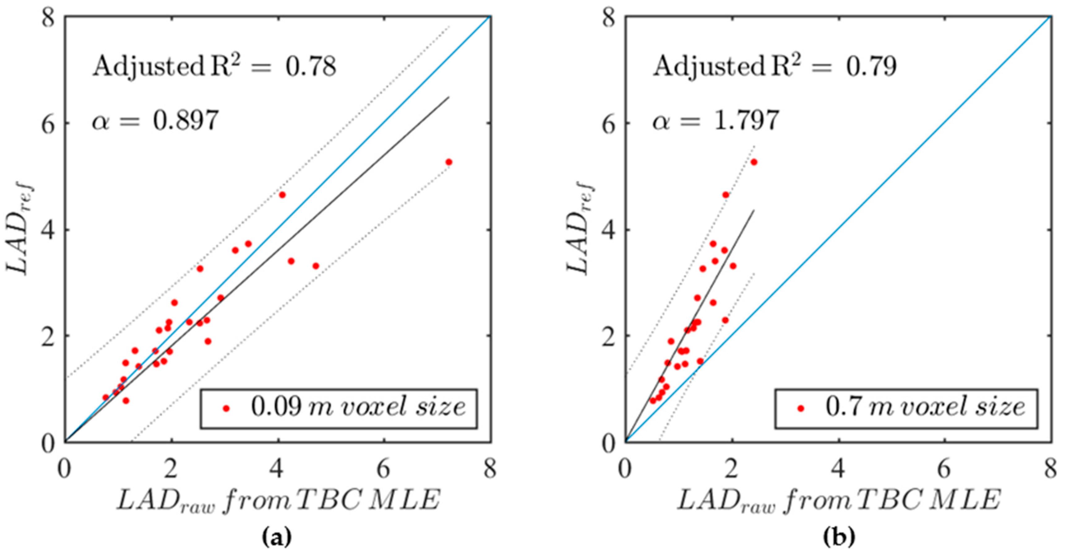
Figure 4 shows some example correlations between raw leaf area densities derived from the FARO data using the TBC MLE estimator at d = 2.5 m and reference leaf area densities for Q. ilex. Subplots (a) and (b) correspond to 9 cm and 70 cm voxel sizes, respectively. A linear fit with a null intercept is reasonable for both voxel sizes, showing that reference and raw LAD were proportional. A regression coefficient $\alpha$ smaller or larger than 1 respectively corresponds to over and underestimation, whereas $\alpha$ equal to 1 corresponds to an unbiased estimator. We found that the 0.09 m voxel size exhibited a small positive bias, whereas the 0.7 m voxel size exhibited a strong negative bias.

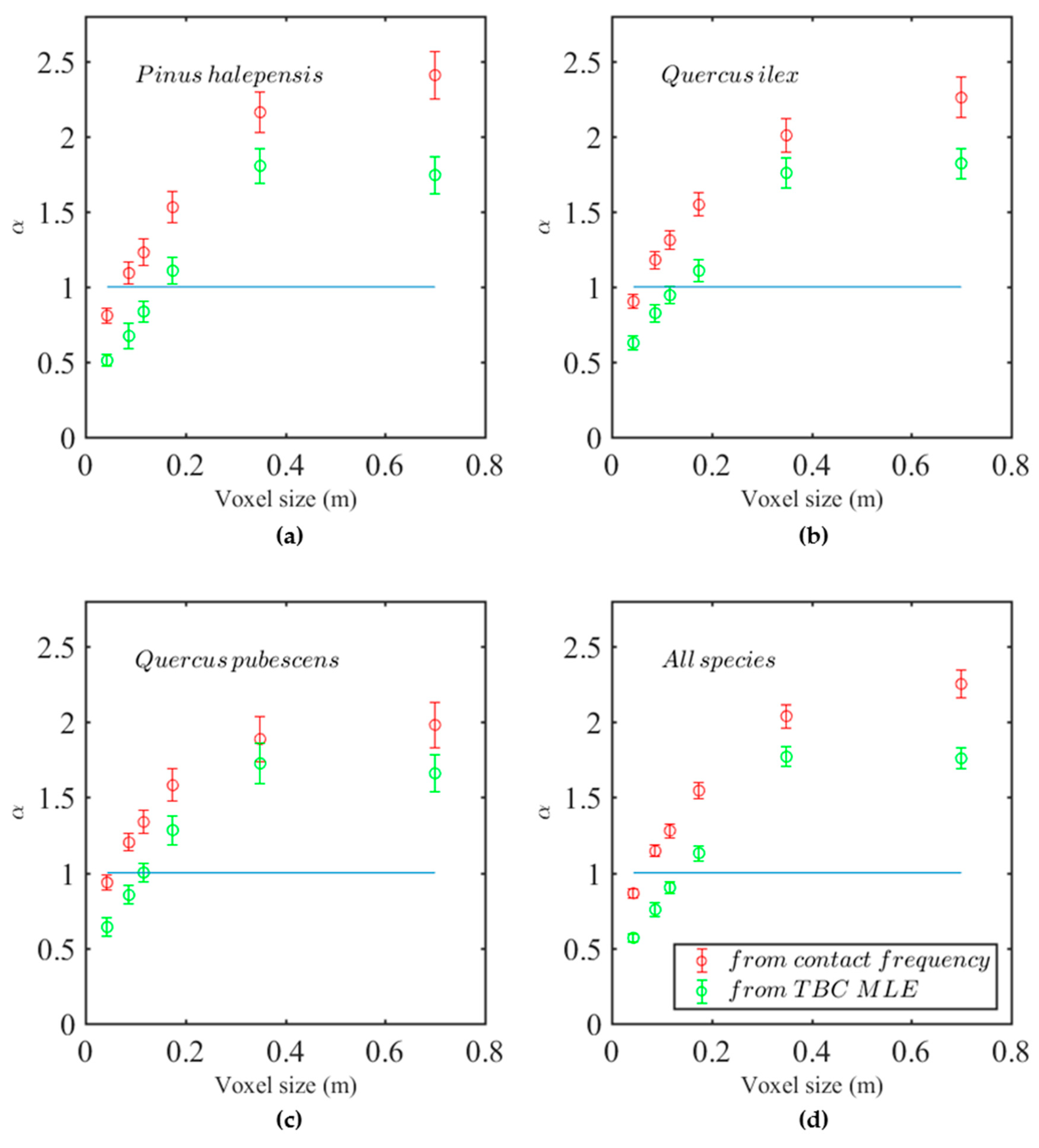
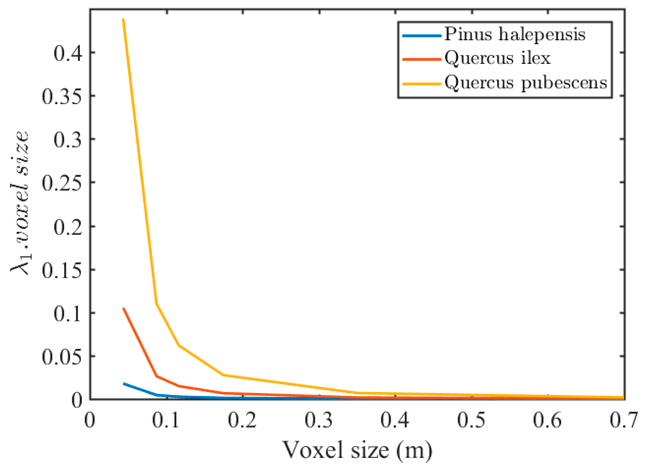
Similar models were fitted for all studied voxel sizes and species, which were the only factors significantly affecting the relationship between raw and reference LAD (Appendix C.2). As the coefficient $\alpha$ often significantly differed from 1, it is later referred to as “calibration coefficient.” The calibration coefficients $\alpha$ are shown in Figure 5 for raw estimators deriving from both Contact Frequency (in red) and TBC MLE (in green). In all cases, the predicted calibration coefficient increased with voxel size until a saturation was reached for voxels larger than 0.35 m, corresponding to a decrease in raw predictions compared to references as voxel size increases. Figure 5a–c shows the calibration coefficients for the three species, whereas all species were combined in Figure 5d. Although statistically significant (Appendix C.2), the differences between species were quantitatively marginal, as the different species exhibited very similar sensitivity to voxel size.

The voxel size was hence clearly the main effect, with a strong increase in calibration coefficient with voxel size for both Contact frequency and TBC MLE.

3.3. Influence of the Distance to Scanner and Subsequent Calibration

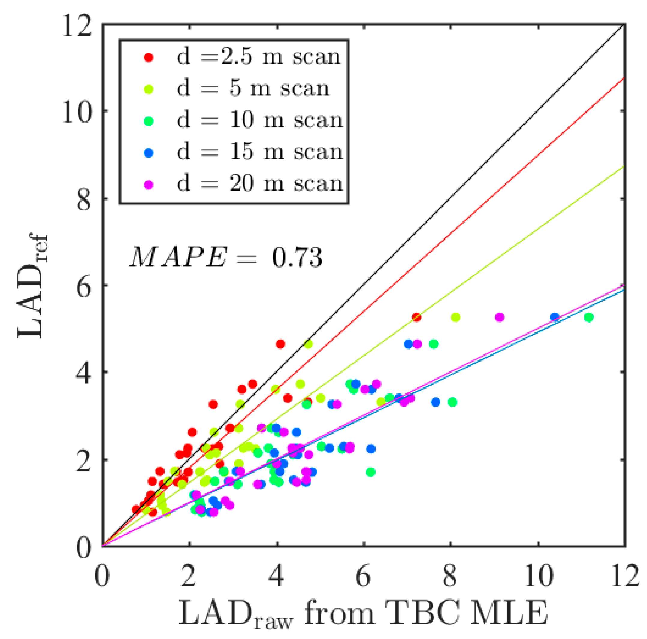
Figure 6 illustrates the influence of the distance to scanner on the raw LAD, for the same case as Figure 4a (i.e., Q. ilex -0.09 m voxel size), the differently coloured dots corresponding to the different distances to scanner. The coloured lines show the slopes of the relationship obtained at the different distances. Obviously, a strong effect of the distance of measurement is observed with the FARO scanner (up to +100% of 2.5 m value for some of the branches), leading to a strong overestimation of the LAD at greater distances.

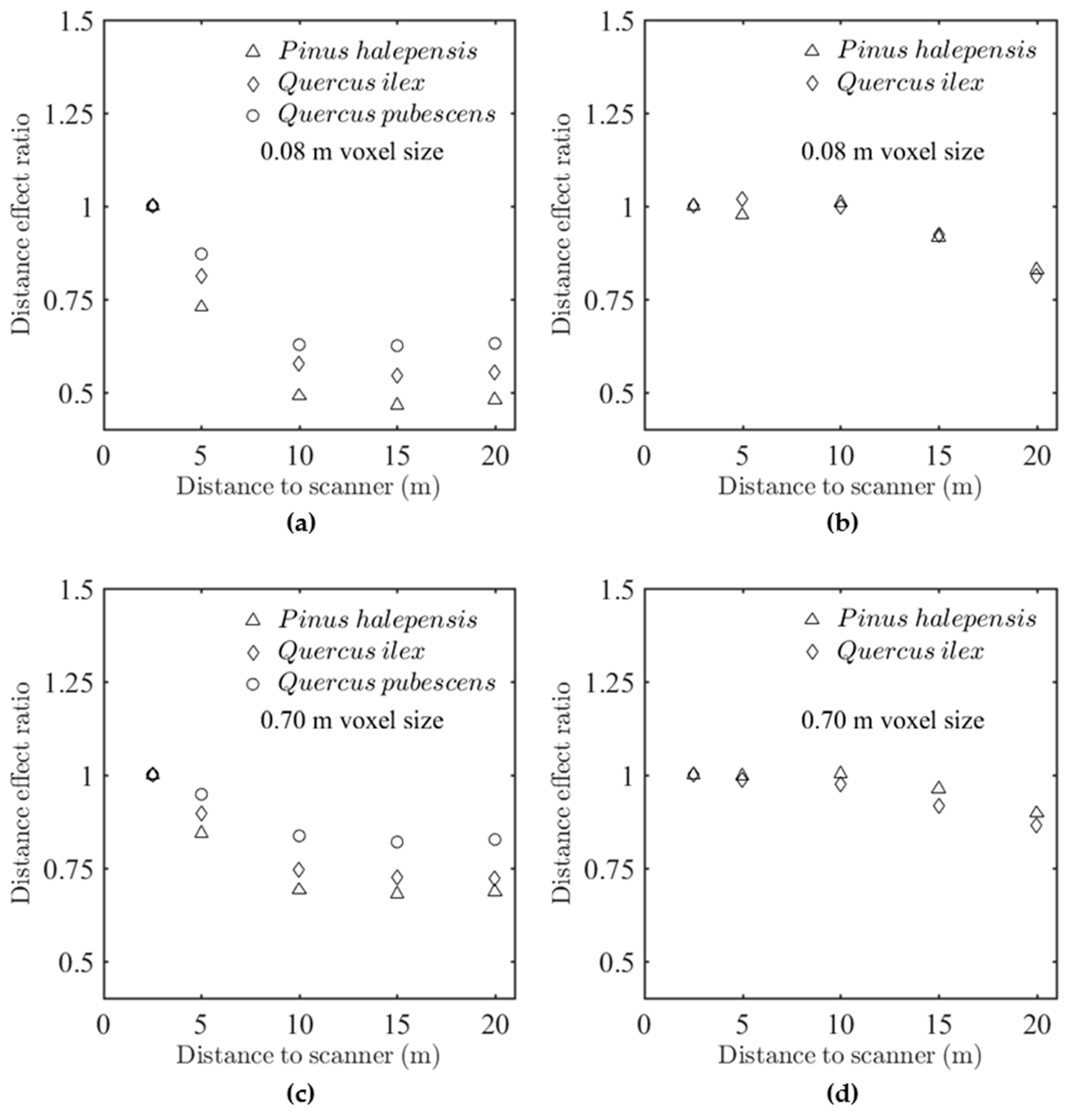
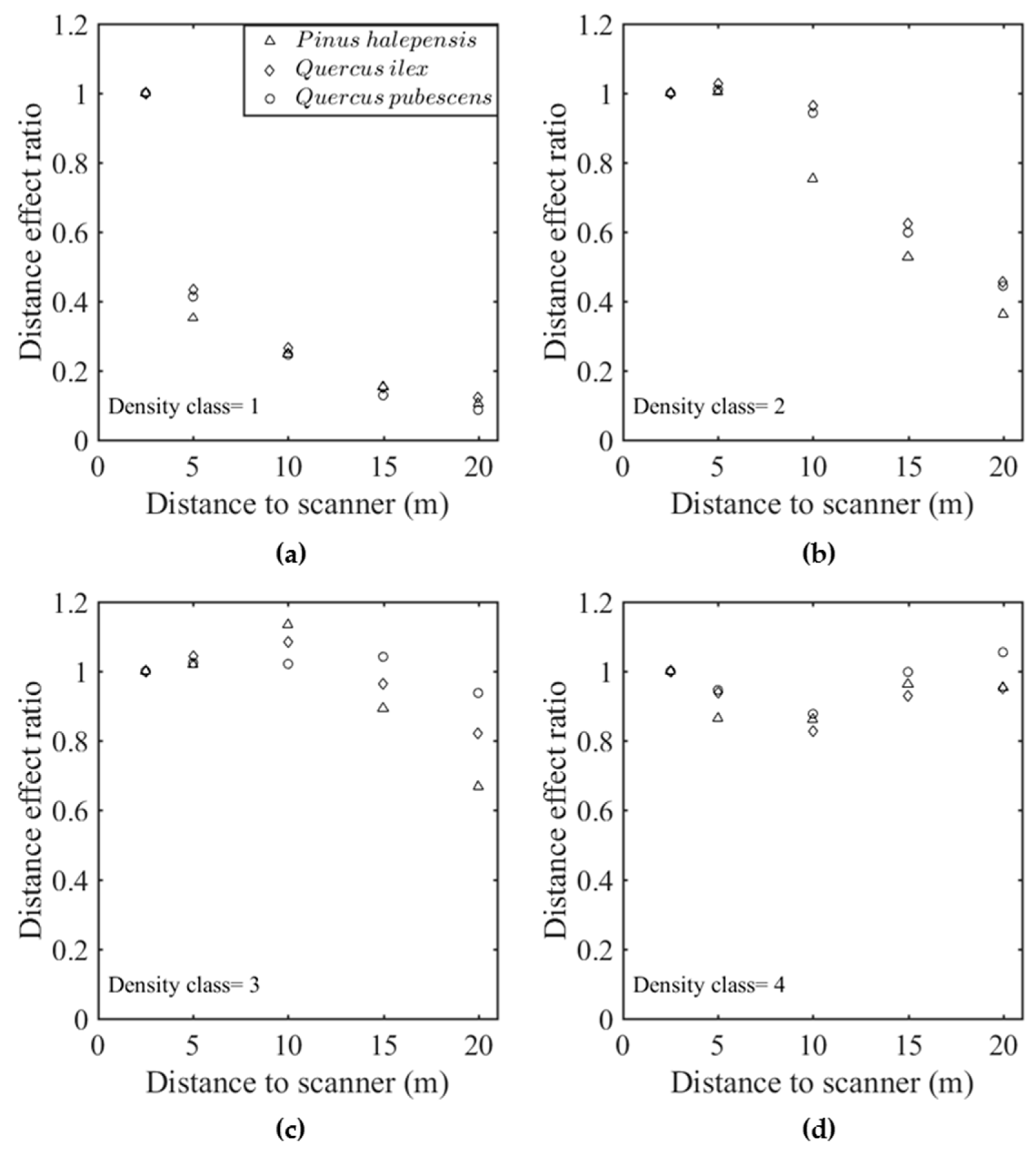
The statistical analysis (Appendix C.3) suggested that this effect of distance to scanner was much lower for the RIEGL than for the FARO scanner and that it was affected by factors such as voxel size and species. Figure 7 shows the “distance effect” ratio, which was defined as the ratio between 2.5 m predictions and the predictions at a given distance d. This ratio was also the calibration factor by which predictions should be multiplied to correct the distance bias (Equation (7)). Subplots (a) and (c) correspond to FARO scanner for two voxel sizes (0.09 and 0.7m), whereas subplots (b) and (d) correspond to the RIEGL scanner for the same voxel sizes. The comparison between the two scanners confirmed that the distance effect was much weaker with the RIEGL than with the FARO system, as suggested in the statistical analysis. However, Figure 7b,d suggest that even the RIEGL system exhibited a small positive bias beyond 10 m, especially for small voxel sizes. For the FARO scanner, the increasing positive bias suggested from Figure 6 was confirmed for all species and the two resolutions. The distance effect thus followed an exponential attenuation for larger voxel sizes. We can observe that Q. pubescens and P. halepensis were the less and the most sensitive species, respectively. The differences between species, although significant (Appendix C.3), were of limited magnitude. The differences induced by voxel size were, much more important, as suggested by the comparison between distance effects in subplot (a) and (c).

Similar trends were observed with the other estimators, with the exception of the estimator derived from the Contact Frequency for which the magnitude of distance effect was slightly smaller.

An in-depth analysis, reported in Appendix E, shows that the bias associated with distance decreased when the vegetation density increased at voxel scale, since the distance effect on estimated LAD was stronger when elements were sparse in a voxel. Such an effect could have been accounted for in the distance model but it would have induced a complex formulation, as the bias correction would have been a function of the overall prediction. This effect was thus neglected in the overall calibration presented in the next subsection.

3.4. Example Calibrated Estimators

In this subsection, we present a selection of calibrated models $LA{D}_{cal}$ developed to correct the raw estimators according to Equations (7)–(9). The models presented in

Table 3. Calibration coefficients for $LA{D}_{raw}$ (Equation (9)) and mean absolute percentage error (MAPE) of the corresponding models.

Attenuation Coefficient	Voxel Size (m)	α (FARO and RIEGL)	$\left[{\mathit{\beta }}_1;{\mathit{\beta }}_2; {\mathit{\beta }}_3\right](\mathbf{Equation} (8\left)\right)$(FARO Only)	MAPE FARO (%)	MAPE RIEGL (%)
CF	0.09	1.15 +/− 0.04	[0.6090; 0.8746;−0.3122]	P. halepensis: 22.5 Q. ilex: 19.7 Q. pubescens: 19.1	21.1 16.7 -
	0.7	2.25 +/− 0.09	[0.7311; 0.5314;−0.2614]	P. halepensis: 20.4 Q. ilex: 25.1 Q. pubescens: 21.8	17.1 19.4 -
${\hat{\mathsf{\Lambda }}}_2$	0.09	0.81 +/− 0.04	[0.5141;1.1216;−0.3362]	P. halepensis: 24.6 Q. ilex: 21.9 Q. pubescens: 27.9	25.1 17.9 -
	0.7	1.85 +/− 0.07	[0.6614;0.6765;−0.2623]	P. halepensis: 20.6 Q. ilex: 22.8 Q. pubescens: 19.4	16.8 15.1 -
$\tilde{\mathsf{\Lambda }}$	0.09	0.76 +/− 0.05	[0.5040;1.0268;−0.3140]	P. halepensis: 27.1 Q. ilex: 24.2 Q. pubescens: 30.8	21.0 13.9 -
	0.7	1.75 +/− 0.07	[0.6873;0.6093;−0.2535]	P. halepensis: 20.6 Q. ilex: 22.1 Q. pubescens: 18.7	16.3 15.9 -

NB. The (small) distance effect of the RIEGL scanner was neglected (i.e., ${\beta }_1=1$ and ${\beta }_2=0$ in Equation (8)).

were developed for both scanners and two voxel sizes (9 and 70 cm) to correct raw estimates obtained using contact frequency method, TBC Beer’s law and TBC MLE approach. The resulting calibrated LAD values, referred to as $LA{D}_{cal}$, included a correction for distance effect when computed for the FARO scanner, whereas this effect was neglected when processing data acquired with the RIEGL scanner (i.e., $f\left(d\right)=1$). The mean absolute percentage errors (MAPE) of the models were systematically smaller with the RIEGL instrument than with the FARO scanner. For the RIEGL scanner, the errors were found to be generally higher for P. halepensis than for Q. ilex.

The calibrated models arising from the most sophisticated attenuation coefficient estimators (${\hat{\mathsf{\Lambda }}}_2$ and $\tilde{\mathsf{\Lambda }}$) exhibited slightly lower errors than the model deriving from the basic contact frequency for the largest voxel size (70 cm) but differences were generally small. When shifting to the small voxel size (9 cm), the errors of the FARO scanner increased for estimators derived from ${\hat{\mathsf{\Lambda }}}_2$ and $\tilde{\mathsf{\Lambda }}$ and remained stable for the contact frequency (CF). Results were more contrasted with the RIEGL scanner, since errors were stable for Q. ilex but increased with P. halepensis when decreasing voxel size.

Overall, the most sophisticated estimators did not perform better than the basic contact frequency (with the exception of the Q. ilex with the RIEGL scanner and the small voxel). This result, which may seem counterintuitive, could be explained by the fact that unbiased estimators often exhibit a larger variability than simpler biased estimators [15], resulting in some cases to a lower residual error at the scale of individual measurements (bias-variance trade-off). This crucial point is discussed in the next section.

Fitting the models on subsets corresponding to species and/or scanners enabled to reduce MAPE values by around 5%. However, corresponding models required a much higher number of coefficients and were thus not considered for further analysis.

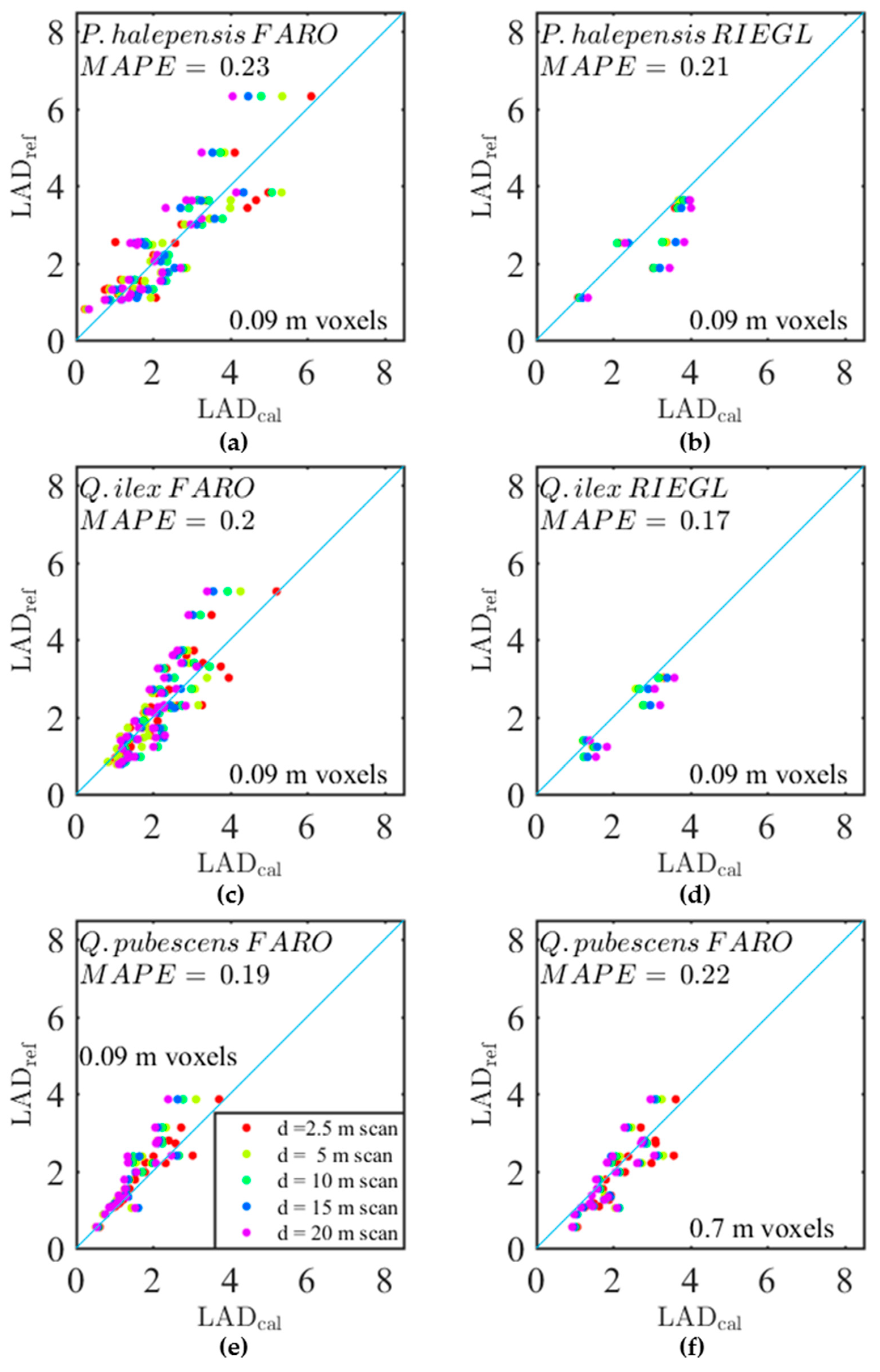
Figure 8 shows LAD predictions after calibration ($LA{D}_{cal}$) for some of the models presented in Table 3. Residual biases of calibrated estimates were low for the FARO instrument, whatever the species or the resolution, with the exception of the branches with highest densities, which were generally underestimated. This underestimation was explained by the fact that the correction for the distance effect was too high in dense branches, because the sensitivity to voxel density of the distance effect was neglected in the calibration model, as explained in Section 3.3. The RIEGL instrument appeared to be more prone to overestimations. This is consistent with the fact that no correction was applied for the positive bias associated with distance in the case of the RIEGL instrument.

4. Discussion

The present work aimed at providing new insights regarding the measurement of leaf area with TLS, from a comparison with destructive laboratory measurements. Our experimental set-up was designed to investigate the impact of several factors affecting LAD estimations through voxel-based methods, which are still poorly understood.

Overall, we observed a strong correlation between the different estimates for LAD and reference measurements. However, these relations were found to be dependent on the type of theoretical estimator (“raw” estimator), the voxel size, the distance to scanner, the scanner type and in a lesser extent, the species. The predictions of the LAD raw estimators were corrected thanks to empirical calibrations.

4.1. Raw Estimations of the LAD

Our results showed that the predictions were sensitive to the type of estimator of the attenuation coefficient. First, we confirmed that the Contact Frequency estimator was negatively biased, at least for short distance to the scanner, as already reported by [20] from measurements, suggested by [12] and theoretically demonstrated by [15]. However, we point out that such bias can be largely overwhelmed by the negative bias associated with large voxels, which might explain the results obtained in Reference [20], who used large voxels (2 m). Second, we found that most bias corrections suggested by [15] were only significant for very small voxels (<9 cm) and long distances (d > 10 m). In these cases, estimators implementing bias corrections exhibited smaller overestimations and higher correlations with reference measurements than the uncorrected estimators, especially the Modified Contact Frequency. This result was promising for further applications of these corrections in the field, where occlusion—which was very limited in our laboratory experiment—leads to numerous voxels which are sampled by a small number of beams, even at short distance to the scanner, especially when fine grids are used for scene discretization (i.e., small voxels).

With the exception of these extreme cases, all raw estimators performed similarly once calibrated, including the Contact Frequency. In particular, our analysis showed a linear relationship between the reference measurements and the Contact Frequency and thus the RDI (because the mean free path is expected to be constant with vegetation density). Such a finding, already reported by [14] in forestry plots, was somehow counterintuitive, as the response function of the LAD to the RDI is expected to follow the Beer-Lambert law ($\approx -\log \left(1-RDI\right)$), which is not linear. This departure from the Beer-Lambert law—which assumes a random distribution of vegetation elements within a voxel—could indicate that the organization of plant elements at small scale would not be random but would rather exhibit some regularity. Indeed, the fact that the absorption (i.e., RDI) was proportional to the leaf area suggests that element clumps tend to be regularly distributed and that self-shading is limited. Hence, this result suggests that TLS voxel-based methods can provide critical data to improve our understanding of plant organization at small scale, which is critical in the context of light interception and transpiration modelling [1,2,3]. It should be recognized, however, that branches were not scanned under a specific orientation (i.e., from above), meaning that scanner beams do not meet the actual direct sun exposure pattern inside vegetation, which limits the interpretation in terms of light interception.

4.2. A Strong Sensitivity of LAD Prediction to Voxel Size, Which Could Mostly Arise from Vegetation Element Distribution

The first calibration step (on short-distance measurements) accounted for remaining sources of biases and uncertainties, once the distance to scanner and voxel sizes were fixed, namely leaf orientation, species, detection capacity of TLS instruments with regards to vegetation structure (beam diameter, element reflectance, sensor sensitivity, partial hit and mixed points). The resulting calibration coefficient was mostly affected by the voxel size. The other factors, such as the species, the instrument or the type of background, were of secondary importance and often not significant. Such a sensitivity to voxel size was already reported in References [19,20,22].

The bias corrections for element size described in Reference [15] slightly reduced this sensitivity when voxel were very small (5–9 cm), when compared to uncorrected estimators. Such finding was in agreement with [22] who described similar element-size effects in small voxels (<10 cm). However, this sensitivity remained strong for both scanners, all species and all estimators, even when theoretical bias corrections were included. This hence supports the assumption that the effect of the voxel size and the subsequent underestimation of LAD observed in largest voxels arose most likely from vegetation heterogeneity, as it was the last remaining source of (negative) bias identified at fixed distance to scanner. It should be noted that [29] found, on the contrary, that LAD predictions increased with voxel size, with variations from 1 to 10 in integrated LAD predictions using the voxel-based canopy profiling method (VCP). This finding can largely be explained by the fact that the VCP method assimilates voxels containing at least one hit to “fully-vegetated” voxels, neglecting the actual vegetation densities in these voxels. As a consequence, the increase in predictions with voxel size observed in Reference [29] may simply arise from a coarser discretization of vegetated volumes. It thus cannot be compared to the voxel-based approaches used in the present paper, as they explicitly accounted for the vegetation density inside voxels.

Noteworthy, it appeared that the short-distance calibration factors reported in the present study were remarkably stable among scanners and backgrounds. Also, this stability holds among species, even for the coniferous species, once a rigorous projection of the pine needles was applied (Appendix A). This suggests that these calibration factors could be used in other studies, provided that the leaf morphology and the TLS instrument did not exhibit large differences with those of the present study.

Finally, this potentially critical influence of vegetation distribution on LAD prediction highlights the problem of methods based on gap fraction, which generally assume that the vegetation distribution is homogeneous in a horizontal layer, to inverse the transmission equation [10,11,30]. Hence, such an approach is theoretically equivalent to the application of a voxel-based method to thin “pancake” voxels with a horizontal extent which encompasses the forest plot, thus potentially leading to LAD underestimations.

4.3. The Sensitivity to Distance to Scanner Led to the Notion of Effective Footprint and Revealed the Existence of Spatial Bias in LiDAR Plot-Scale Estimations

In addition to these variations at 2.5 m, a strong effect of distance was revealed for the FARO instrument and in a smaller extent for the RIEGL instrument. The farther the scanner was from the vegetation, the higher the estimated LAD was. We would like to highlight the importance of this finding, which reveals the presence of equally large spatial biases in measurements at the scale of a vegetation scene (e.g., forest plot) when raw estimates are not corrected for the distance effect, which is the case of most studies. Indeed, plot-scale or tree-scale measurements combine various estimations done at several distances to scanner, especially when the canopy is high. As a result, an estimated LAI of 2 in a 5-m or in a 20-m high canopy might correspond to considerably different actual LAI. As for the voxel-size effect, such a distance effect also leads to bias in gap fraction estimates, as their computation rely on the same theoretical basis. Hence, they should also be corrected for distance effect.

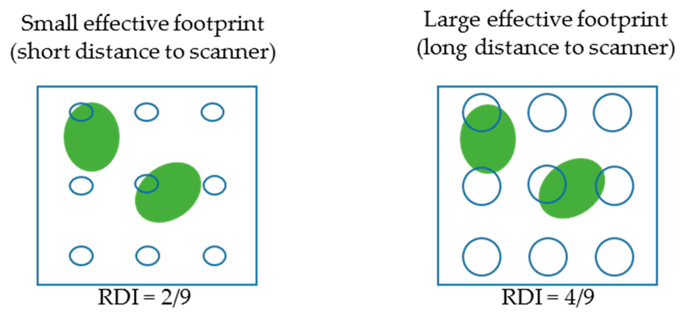
As explained in the introduction, this distance effect could be explained by an increase in the hit probability resulting from the increase of laser footprint with distance to scanner, induced by beam divergence ([12]). Indeed, when beam diameters increase with distance to scanner, beams lose their ability to pass through vegetation elements without triggering a hit, leading to higher RDI and hence, LAD estimates (Figure 9). In other word, vegetation elements are “seen” by the scanner bigger than they actually are, as returns can be registered even when the beam centre lines do not intercept any elements. Another explanation to the sensitivity to distance might have been the decay of beam number in voxels, which causes a positive theoretical bias in uncorrected estimates [15]. However, we observed similar increases with distance when this theoretical bias was corrected, suggesting that the beam divergence was the main cause of observed sensitivity to distance. The distance effect was found to slightly vary among species (Figure 7), the effect being stronger for species with smaller vegetation elements (pine needles) than with larger leaves. This was consistent with the above explanation, as the relative increase in probability of interception was found to be bigger for fine than for large elements. The specifications provided by the instrument manufacturers entail to estimate a theoretical footprint at the exit (beam diameters equal to 6.5 mm and 2.25 mm for the RIEGL and the FARO, respectively) and at further distances (beam divergence equal to 0.35 mrad and 0.19 mrad for the RIEGL and the FARO, respectively). From these theoretical specifications, the footprint of the RIEGL at 2.5 m (42.7 mm²) should be much larger than the one of the FARO (5.8 mm²), so that the raw estimates of the FARO should have been much lower than those of the RIEGL. This contradicts the results observed at 2.5 m (calibration coefficient not being sensitive to the instrument) and suggests that the raw estimates do not only reflect the size of the theoretical footprint but also other characteristics of the scanner and how beams interact with vegetation elements (element reflectance, sensor sensitivity, partial hit management).

In practice, a beam diameter of a given size does not mean that a scanner can detect vegetation within this whole footprint. Indeed, a hit is registered only when the intensity of the return is higher than a given threshold [11], so that not all partial hits are detected. To facilitate data interpretation, we suggest the notion of effective footprint (or equivalently effective beam size), which would be the mean footprint area within which vegetation elements are actually detected in a given voxel. This effective footprint would depend of the beam diameter but also of the sensor detection threshold, the return intensity and vegetation element properties and is expected to be smaller than the actual footprint of the scanner. Our short-distance analyses suggest that both the FARO and the RIEGL exhibited similar effective footprints at d = 2.5 m, since the calibration coefficient obtained with both instruments were similar, despite of the differences in theoretical footprints (possibly because of a lower detection threshold of the RIEGL, which might have offset its larger footprint). The distance effect pattern suggested that the effective footprint of the RIEGL was more or less constant with distance up to 10 m, before slightly increasing at further distances. Conversely, the effective footprint of the FARO strongly increased before 10 m and was constant at further distances. A physical modelling of such an effective footprint is not straightforward, even if some physical bases were provided in Reference [11]. However, the physical approach is limited with scanner such as the FARO, as several factors affect the registered value of phase-shift scanner intensity, such as temperature [31] and shooting direction in the different phases. The methodology presented here provided a promising alternative to calibrate the sensitivity to distance.

The magnitude of the distance effect decreases with voxel size (Figure 7), which was somehow counterintuitive. This observation could arise from the heterogeneous structure of the vegetation, as suggested by the following mechanism. Smaller voxels lead to more frequent “empty” voxels, as their size approaches the size of gaps between shoots in a branch. Hence, the raw LAD distribution is wider on a finer grid. As shown in Appendix E, the distance effect was much stronger in voxels with low density, whereas it was smaller and fairly constant at medium and high densities. As a result, the changes in raw LAD distribution due to smaller voxels (in particular the increase in frequency of low density voxels) induce a higher frequency of voxels with stronger distance effect and hence a slightly stronger overall distance effect (at branch scale) with small voxels.

4.4. Calibrated Estimator Performance

Overall, calibrated raw LAD estimates exhibited lower error with the RIEGL than with the FARO scanner. Hence, the RIEGL obtained the lowest errors with Q. ilex for all voxel sizes (about 15%). The better performance of the RIEGL instrument (despite no correction for distance was applied) might be explained by a better management of mixed pixels and a lower level of noise with time-of-flight than with phase-shift scanners. Indeed, the RIEGL scanner registers the 3D coordinates of the location where the return intensity was the highest, whereas the FARO scanner combines the information arising from multiple phase shifts (3 wavelengths for the FARO), leading to the registration of a hit position located within the shortest and longest distances at which intensity was returned, which does not necessarily correspond to the location where the actual vegetation element is. Hence, the FARO might be more subject to hit misplacement. However, the performance of the RIEGL scanner was generally lower with P. halepensis compared to the FARO scanner, especially for the smallest voxel sizes (<15 cm).

Overall, with the exception of Q. ilex, a decrease in voxel size led to higher errors in LAD predictions with both scanners, even with theoretically TBC estimators (Table 3). It has been demonstrated [15] that the variability in raw estimates sharply increased with decreasing number of beams and number of vegetation elements within a voxel, leading to large measurements errors. The increase in errors observed below 10 cm suggests that the overall measurement accuracy at branch scale was affected by the measurement errors resulting from random effects occurring at small scale. Indeed, 10 cm appeared as a good compromise between limited error arising from uncertainties of measurements in small voxels and an adequate representation of spatial heterogeneity. It is important to notice, however, that similar measurement error can be achieved in larger voxels, provided that a relevant calibration was applied.

The lower performance of the more sophisticated (TBC) estimators when applied to the FARO scanner at small voxel size suggests that these estimators were more sensitive to measurement error and noise than simple estimators (i.e., CF). This could be interpreted as an example of the bias-variance trade-off. Indeed, sophisticated estimators were theoretically unbiased, meaning that their expectation over a large number of trials was closer to the actual value. [15] showed that their variance was the smallest that could be expected from any unbiased estimators (since they reached the Cramer-Rao bound, see [15]) but also that this variance was high (leading to 95% confident interval as large as 100% of the expectation when beam number was low and vegetation elements were large). Moreover, the TBC estimators do not account for vegetation heterogeneity, a major source of bias as suggested in the present paper. As a result, it is not surprising that once calibrated at the scale of interest (here the branch), more basic estimators with smaller variance (such as the basic contact frequency approach) were more robust to noise and led to smaller errors than the TBC estimator. Another potential cause of limited performance of the bias-corrected estimator, might be the fact that the spatial arrangement of vegetation would not be random at small scale, as suggested in Section 4.1.

These findings, based on detailed laboratory data, highlight the critical need for detailed field data and actual TLS data to validate or invalidate finding arising from theory and simulations.

4.5. Recommendations and Further Work

Our study confirmed a strong sensitivity of the LAD estimation to discretization arising from vegetation heterogeneity and revealed a strong distance effect which, if not corrected, can lead to large spatial biases in LiDAR plot-scale estimates. The observed variations among tested scanners showed that emission pattern and properties of beams from LiDAR instruments play an important role in results and in spatial robustness of estimators. We thus recommend that these mechanisms are accounted for in further studies addressing the estimation of LAD with TLS. These recommendations apply not only to voxel-based methods but also to gap fraction approaches.

The method presented in the present study (calibration based on experimental tests on branches) could be applied to other species, estimators and instruments as a first step to improve LAD estimations by the use of calibration functions. The evaluation/calibration procedure developed in this study can be replicated because it is easily reproducible and reasonably time-consuming (1 week per species). In addition, the same calibration could be applied to species exhibiting close vegetation structure. This method can be seen as a fast approach to characterize bias occurring in LAD estimations.

It is however important to recognize that such laboratory studies do not replace experimental approaches at plant [12] or stand scales [14], as additional issues, such as determining the leaf fraction or accounting for occlusion should be tackled to assess reliable LAD [19]. Occlusion was avoided on purpose in this study to ensure detection of vegetation elements and achieve corrections of biases related to vegetation heterogeneity and scanner properties only. The occurrence of occlusion on field might hence limit reliability of our estimations, even though this work deals with some occlusion issues. Indeed, tested TBC estimators theoretically account for decrease in number of beams used for voxel sampling, which is a major drawback of occlusion. In addition, small voxel sizes used in this study (e.g., 0.09 m) enable an accurate pinpointing of potentially occluded areas. Nevertheless, other biases (i.e., heterogeneous sampling of voxel or totally occluded areas inside tree crowns) are not addressed as it was not the purpose of this work. Large scale specific experiments at tree or stand scale are also required to evaluate the calibration derived from laboratory experiments.

Finally, the RIEGL scanner was used in this experiment similarly as a single return instrument, that is, neglecting further impacts (second, third and fourth returns) which only represent 4% of total registered returns. This low percentage of multiple returns was mainly due to the background characterized by an obstacle-free distance of at least 100 m in the scan direction when the RIEGL scanner was used (see Section 2.1). However, in field measurements, a significant increase in the number of multiple returns is expected due to the surrounding vegetation. Considering first returns only results in an underestimation of voxel transmittance, that is, an overestimation of RDI and LAD. Indeed, in that case, for each return, the vegetation is implicitly assumed to fully intercept the laser beam or, in other words, to cover the whole beam area. Most of the time, part of the beam energy is not intercepted and the leaf area responsible for an echo detection is smaller than the whole footprint area. It has been demonstrated that using multiple returns information enhanced LAD estimates and that the smaller the leaves, the more significant the improvement is [13]. To take into account this information several strategies have been proposed to weight echoes when computing the RDI. Weighting can be based either on echo intensities [19] or on the number [13] or on the number and rank [32], of the echoes belonging to the same laser beam. However, taking into account partial interceptions remains challenging due to the numerous factors that influence echo intensity and also because information about the amount of energy remaining in the laser beam after the last echo, if any, is always missing.

When dealing with partial interceptions by using multiple returns information, raw LAD estimates and, consequently, appropriate calibration coefficients can thus depend on voxel environment. For these reasons, it should be more effective and accurate to assess and use the calibration coefficients obtained with the proposed approach, considering first returns only when working with field measurements.

5. Conclusions

This work consolidates and extends previous knowledge regarding the use of TLS to retrieve reliable LAD (and LAI) estimates. From our laboratory experiments, we tested recent theoretical developments regarding the estimation of LAD through voxel-based approaches and identified some important sources of bias in measurements. Our analyses permitted to disentangle the biases arising from sampling, vegetation arrangement and scanner specifications. We provided evidences that the most significant biases arose from both the distribution of vegetation element at small scale (voxel-size effect) and some variations in the effective footprint of scanners (distance effect). This “effective footprint” is the footprint of a beam in which specific vegetation elements can effectively be detected at a given distance to scanner. Even for theoretically unbiased estimators, the correction of these effects was shown to be mandatory and provided LAD estimates within 20% error to the destructive references of the present experiment.

Regarding the appropriate voxel size, our study showed that the voxels smaller than 10 cm led to increasing measurement errors (because of random processes occurring below this scale) and that these measurements errors were fairly constant for larger voxel size, provided that an appropriate calibration coefficient was applied.

We provided a method for the calibration of theoretical estimators. Because tested TLS are widely used on field campaign on similar vegetation and because measurements at tree scale encompass voxels at various distances from scanner, this method provides LAD estimates that are less biased when applied at plant or plot scale in the field. Calibration functions can be readily applied when vegetation and TLS are similar to those of the present study but should be used with caution in other cases.

References

1. Norman, J.M.; Campbell, G.S. Canopy structure. In Plant Physiological Ecology: Field Methods and Instrumentation; Pearcy, R.W., Ehleringer, J.R., Mooney, H.A., Rundel, P.W., Eds.; Springer: Dordrecht, The Netherlands, 1989; pp. 301–325. ISBN 978-94-009-2221-1. [Google Scholar]
2. Simioni, G.; Marie, G.; Huc, R. Influence of vegetation spatial structure on growth and water fluxes of a mixed forest: Results from the NOTG 3D model. Ecol. Model. 2016, 328, 119–135. [Google Scholar] [CrossRef]
3. Vezy, R.; Christina, M.; Roupsard, O.; Nouvellon, Y.; Duursma, R.; Medlyn, B.; Soma, M.; Charbonnier, F.; Blitz-Frayret, C.; Stape, J.L.; et al. Measuring and modelling energy partitioning in canopies of varying complexity using MAESPA model. Agric. For. Meteorol. 2018, 253–254, 203–217. [Google Scholar] [CrossRef]
4. Vierling, K.T.; Vierling, L.A.; Gould, W.A.; Martinuzzi, S.; Clawges, R.M. Lidar: Shedding new light on habitat characterization and modeling. Front. Ecol. Environ. 2008, 6, 90–98. [Google Scholar] [CrossRef]
5. Keane, R. Wildland Fuel Fundamentals and Applications; Springer International Publishing: Cham, Switzerland, 2015. [Google Scholar]
6. Jonckheere, I.; Fleck, S.; Nackaerts, K.; Muys, B.; Coppin, P.; Weiss, M.; Baret, F. Review of methods for in situ leaf area index determination Part I. Theories, sensors and hemispherical photography. Agric. For. Meteorol. 2004, 121, 19–35. [Google Scholar] [CrossRef]
7. Bréda, N.J.J. Ground-based measurements of leaf area index: A review of methods, instruments and current controversies. J. Exp. Bot. 2003, 54, 2403–2417. [Google Scholar] [CrossRef] [PubMed]
8. Weiss, M.; Baret, F.; Smith, G.J.; Jonckheere, I.; Coppin, P. Review of methods for in situ leaf area index (LAI) determination Part II. Estimation of LAI, errors and sampling. Agric. For. Meteorol. 2004, 121, 37–53. [Google Scholar] [CrossRef]
9. Chen, J.M.; Cihlar, J. Plant canopy gap-size analysis theory for improving optical measurements of leaf-area index. Appl. Opt. 1995, 34, 6211–6222. [Google Scholar] [CrossRef] [PubMed]
10. Jupp, D.L.B.; Culvenor, D.S.; Lovell, J.L.; Newnham, G.J.; Strahler, A.H.; Woodcock, C.E. Estimating forest LAI profiles and structural parameters using a ground-based laser called ’Echidna? Tree Physiol. 2009, 29, 171–181. [Google Scholar] [CrossRef] [PubMed]
11. Zhao, K.; García, M.; Liu, S.; Guo, Q.; Chen, G.; Zhang, X.; Zhou, Y.; Meng, X. Terrestrial lidar remote sensing of forests: Maximum likelihood estimates of canopy profile, leaf area index, and leaf angle distribution. Agric. For. Meteorol. 2015, 209–210, 100–113. [Google Scholar] [CrossRef]
12. Béland, M.; Widlowski, J.L.; Fournier, R.A.; Cote, J.F.; Verstraete, M.M. Estimating leaf area distribution in savanna trees from terrestrial LiDAR measurements. Agric. For. Meteorol. 2011, 151, 1252–1266. [Google Scholar] [CrossRef]
13. Grau, E.; Durrieu, S.; Fournier, R.; Gastellu-etchegorry, J.; Yin, T. Estimation of 3D vegetation density with Terrestrial Laser Scanning data using voxels. A sensitivity analysis of influencing parameters. Remote Sens. Environ. 2017, 191, 373–388. [Google Scholar] [CrossRef]
14. Pimont, F.; Dupuy, J.L.; Rigolot, E.; Prat, V.; Piboule, A. Estimating leaf bulk density distribution in a tree canopy using terrestrial LiDAR and a straightforward calibration procedure. Remote Sens. 2015, 7, 7995–8018. [Google Scholar] [CrossRef]
15. Pimont, F.; Allard, D.; Soma, M.; Dupuy, J.L. Estimators and confidence intervals for plant area density at voxel scale with T-LiDAR. Remote Sens. Environ. 2018, 215, 343–370. [Google Scholar] [CrossRef]
16. Durrieu, S.; Allouis, T.; Fournier, R.; Véga, C.; Albrech, L. Spatial quantification of vegetation density from terrestrial laser scanner data for characterization of 3D forest structure at plot level. In Proceedings of the SilviLaser 2008, Edinburgh, UK, 17–19 September 2008; pp. 325–334. [Google Scholar]
17. Hosoi, F.; Omasa, K. Factors contributing to accuracy in the estimation of the woody canopy leaf area density profile using 3D portable lidar imaging. J. Exp. Bot. 2007, 58, 3463–3473. [Google Scholar] [CrossRef] [PubMed] [Green Version]
18. Bailey, B.; Mahaffee, W. Rapid, high-resolution measurement of leaf area and leaf orientation using terrestrial LiDAR scanning data. Meas. Sci. Technol. 2017, 28, 6. [Google Scholar] [CrossRef]
19. Béland, M.; Widlowski, J.L.; Fournier, R.A. A model for deriving voxel-level tree leaf area density estimates from ground-based LiDAR. Environ. Model. Softw. 2014, 51, 184–189. [Google Scholar] [CrossRef]
20. Bailey, B.N.; Mahaffee, W.F. Rapid measurement of the three-dimensional distribution of leaf orientation and the leaf angle probability density function using terrestrial LiDAR scanning. Remote Sens. Environ. 2017, 194, 63–76. [Google Scholar] [CrossRef]
21. Seielstad, C.; Stonesifer, C.; Rowell, E.; Queen, L. Deriving fuel mass by size class in Douglas-fir (Pseudotsuga menziesii) using terrestrial laser scanning. Remote Sens. 2011, 3, 1691–1709. [Google Scholar] [CrossRef]
22. Béland, M.; Baldocchi, D.D.; Widlowski, J.L.; Fournier, R.A.; Verstraete, M.M. On seeing the wood from the leaves and the role of voxel size in determining leaf area distribution of forests with terrestrial LiDAR. Agric. For. Meteorol. 2014, 184, 82–97. [Google Scholar] [CrossRef]
23. Ruel, J.J.; Ayres, M.P. Jensen’s inequality predicts effects of environmental variation. Tree 1999, 5347, 361–366. [Google Scholar] [CrossRef]
24. Pimont, F.; Dupuy, J.L.; Caraglio, Y.; Morvan, D. Effect of vegetation heterogeneity on radiative transfer in forest fires. Int. J. Wildland Fire 2009, 18, 536–553. [Google Scholar] [CrossRef]
25. Hebert, M.; Krotkov, E. 3D measurements from imaging laser radars: How good are they? Image Vis. Comput. 1992, 10, 170–178. [Google Scholar] [CrossRef]
26. Newnham, G.; Armston, J.; Muir, J.; Goodwin, N.; Tindall, D.; Culvenor, D.; Püschel, P.; Nyström, M.; Johansen, K. Evaluation of Terrestrial Laser Scanners for Measuring Vegetation Structure; CSIRO Sustainable Agriculture Flagship; CSIRO: Canberra, Australia, 2012; pp. 1–32. [Google Scholar] [CrossRef]
27. Leica Geosystems Cyclone Pointcloud Export Format—Description of ASCII. Ptx Format. Available online: http://w3.leica-geosystems.com/kb/?guid=5532D590-114C-43CD-A55F-FE79E5937CB2 (accessed on 22 June 2018).
28. Wilson, J.W. Inclined point quadrats. New Phytol. 1960, 59, 1–7. [Google Scholar] [CrossRef]
29. Li, S.; Dai, L.; Wang, H.; Wang, Y.; He, Z.; Lin, S. Estimating leaf area density of individual trees using the point cloud segmentation of terrestrial LiDAR data and a voxel-based model. Remote Sens. 2017, 9, 1202. [Google Scholar] [CrossRef]
30. Zhao, F.; Yang, X.; Schull, M.A.; Román-Colón, M.O.; Yao, T.; Wang, Z.; Zhang, Q.; Jupp, D.L.B.; Lovell, J.L.; Culvenor, D.S.; et al. Measuring effective leaf area index, foliage profile, and stand height in New England forest stands using a full-waveform ground-based lidar. Remote Sens. Environ. 2011, 115, 2954–2964. [Google Scholar] [CrossRef]
31. Errington, A.F.C.; Daku, B.L.F. Temperature compensation for radiometric correction of terrestrial LiDAR intensity data. Remote Sens. 2017, 9, 356. [Google Scholar] [CrossRef]
32. Vincent, G.; Antin, C.; Laurans, M.; Heurtebize, J.; Durrieu, S.; Lavalley, C.; Dauzat, J. Mapping plant area index of tropical evergreen forest by airborne laser scanning. A cross-validation study using LAI2200 optical sensor. Remote Sens. Environ. 2017, 198, 254–266. [Google Scholar] [CrossRef]
Figure 1. Example branches set-up in laboratory: (a) Leaf-on Q. pubescens branch; (b) Half-foliated Q. pubescens branch; (c) Scanning leaf-on Q. ilex branch; (d) Leaf-off Q. ilex branch.
Remotesensing 10 01580 g001
Figure 2. Mean number of beams reaching a single voxel as a function of its size, for FARO scans. Coloured series correspond to the different distances between scanner and vegetated volumes, from 2.5 to 20 m.
Remotesensing 10 01580 g002
Figure 3. Comparison between predictions of the L A D r a w corresponding to the different estimators of the attenuation coefficients (Table 2 for details) for Q. pubescens: (a) From Contact Frequency as a function of TBC MLE, with a distance to scanner of 5 m and a voxel size of 9 cm; (b) From TBC Beer-Lambert as a function of TBC MLE, with a distance to scanner of 5 m and a voxel size of 9 cm; (c) Same as (a) but for a voxel size of 70 cm; (d) Same as (b) but for a voxel size of 70 cm; (e) From usual Beer-Lambert, as a function of TBC Beer-Lambert, with a distance to scanner of 20 m and two voxel size (4 and 9 cm); (f) From Modified Contact Frequency (MCF), as a function of TBC MLE, with a distance to scanner of 20 m and two voxel size (4 and 9 cm). Blue line is 1:1 line. This figure illustrates some of the similarities and differences between the predictions arising from the different raw estimators.
Remotesensing 10 01580 g003
Figure 4. Comparison between L A D r a w (derived from Λ ˜ ) and reference measurements L A D r e f , when the FARO scanner was at short distance of Q. ilex (d = 2.5 m), for two voxel sizes (a) 0.09 m; (b) 0.7 m. Red dots represent each individual leaf samples (leaf on and half defoliated). The blue lines represent the no bias line. The black lines represent the linear fit (with slope α , which is the calibration coefficient defined in Equation (6)). Black dotted lines represent the 95% confidence interval of the prediction. This figure illustrates that a change in voxel size induces a shift in the slope of the relationship between raw estimations and reference measurements.
Remotesensing 10 01580 g004
Figure 5. Calibration factors α for L A D r a w (Equation (6)) as a function of voxel size for (a) P. halepensis, (b) Q. ilex, (c) Q. pubescens and (d) for all species mixed. α = 1 (blue line) corresponds to the no-bias line, whereas correction factors α < 1 and α > 1 correspond to respectively over and under estimation. The Contact Frequency estimators are in red. The TBC MLE estimators are in green. Vertical bars are 95% confidence intervals for each regression coefficient α . This figure illustrates that a change in voxel size) induces a shift in the slope of the relationship between raw estimations and reference measurements.
Remotesensing 10 01580 g005
Figure 6. Comparison between L A D r a w , derived from the TBC MLE ( Λ ˜ ) and reference measurements L A D r e f for Q. ilex with the 0.09 voxel size. The different coloured dots correspond to various distances d to scanner. The black line represents the no bias line. Other coloured lines correspond to regression between estimates and reference. This figure illustrates that the prediction of the FARO scanner was highly sensitive to distance to the scanner, as raw LAD increased with this distance. MAPE is the Mean Absolute Percentage Error.
Remotesensing 10 01580 g006
Figure 7. Sensitivity to distance to scanner of L A D r a w derived from the TBC MLE ( Λ ˜ ), expressed by the “distance effect ratio” (Equation (7)), which was the ratio between L A D r a w value at 2.5 m to L A D r a w values at a distance d (m). Distance effect ratios are shown for the different scanners and two voxel sizes: (a) FARO scanner, voxel size = 9 cm; (b) RIEGL scanner, voxel size = 9 cm; (c) FARO scanner, voxel size = 70 cm; (d) RIEGL scanner, voxel size = 70 cm. This figure shows that the distance effects were much smaller with the RIEGL than with the FARO scanners. The distance effects are sensitive to voxel size and, in a lower extent, to the species.
Remotesensing 10 01580 g007
Figure 8. Reference measurements against calibrated estimators L A D c a l derived from λ C F for the three species for (a) P. halepensis with 0.09 cm voxel and FARO scanner; (b) Pinus halepensis with 0.09 m voxel and RIEGL scanner; (c) Q. ilex with 0.09 m voxel and FARO scanner; (d) Q. ilex with 0.09 m voxel and RIEGL scanner; (e) Q. pubescens with 0.09m voxel and FARO scanner; (f) Q. pubescens with 0.09 m voxel and FARO scanner. This figure shows how some of calibration models presented in Table 3 performed against reference measurements.
Remotesensing 10 01580 g008
Figure 9. Impact of the size of the effective footprint on RDI estimates. The increase in effective footprint (blue circles) associated with longer distance to scanner (RDI increasing from 2/9 to 4/9).
Remotesensing 10 01580 g009