Observation of CO2 Regional Distribution Using an Airborne Infrared Remote Sensing Spectrometer (Air-IRSS) in the North China Plain

1
Key Laboratory of Environmental Optics and Technology, Anhui Institute of Optics and Fine Mechanics, Chinese Academy of Sciences, Hefei 230031, China
2
University of Science and Technology of China, Hefei 230026, China
3
CAS Center for Excellence in Urban Atmospheric Environment, Institute of Urban Environment, Chinese Academy of Sciences, Xiamen 361021, China
4
University of Chinese Academy of Sciences, Beijing 100049, China
*
Authors to whom correspondence should be addressed.
Remote Sens. 2019, 11(2), 123; https://doi.org/10.3390/rs11020123
Submission received: 12 November 2018
/
Revised: 7 January 2019
/
Accepted: 8 January 2019
/
Published: 10 January 2019
(This article belongs to the Special Issue Application of Ground and Space Based Remote Sensing for Air Pollution)
Abstract
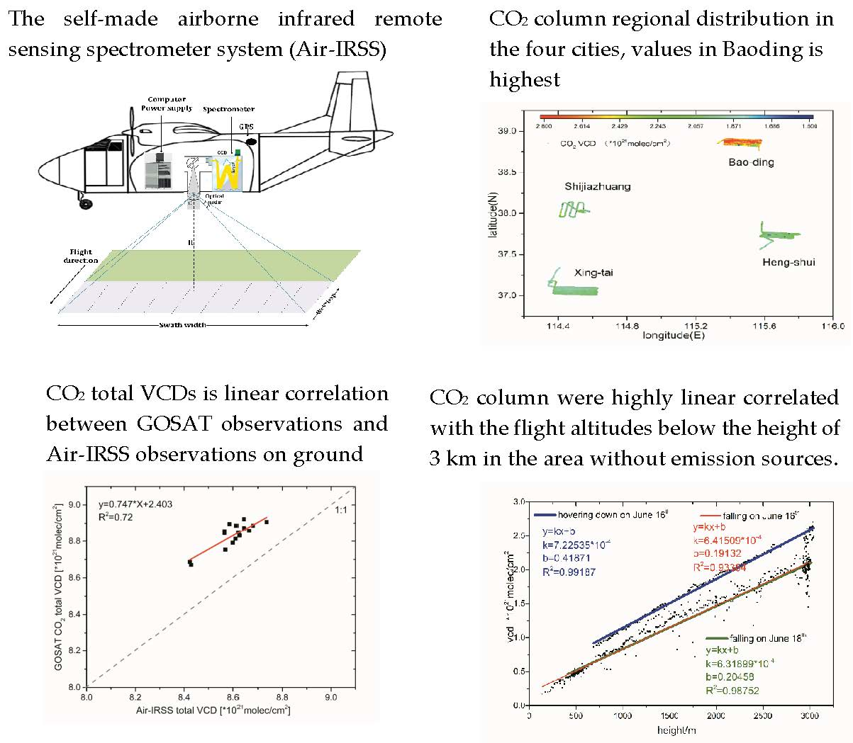
:Carbon dioxide (CO2) is one of the most important anthropogenic greenhouse gases (GHG) and significantly affects the energy balance of atmospheric systems. Larger coverage and higher spatial resolution of CO2 measurements can complement the existing in situ network and satellite measurements and thus improve our understanding of the global carbon cycle. In this study, we present a self-made airborne infrared remote sensing spectrometer (Air-IRSS) designed to determine the regional distribution of CO2. The Air-IRSS measured CO2 in the spectral range between 1590 and 1620 nm at a spectral resolution of 0.45 nm and an exposure time of 1 s. It was operated onboard an aircraft at a height of 3 km with a velocity of 180 km/h, and a spatial resolution of 50.00 m × 62.80 m. Weighting function modified differential optical absorption spectroscopy (WFM-DOAS) was used to analyze the measured spectra. The results show that the total uncertainty estimated for the retrieval of the CO2 column was 1.26% for airborne measurements over a large region, and 0.30% for a fixed point, such as power points or factories. Under vibration-free static conditions, the on-ground Air-IRSS observations can adequately reproduce the variations observed by Greenhouse Gases Observing Satellite (GOSAT) with a correlation coefficient (r) of 0.72. Finally, we conducted an airborne field campaign to determine the regional distribution of CO2 over the North China Plain. The regional distribution of CO2 columns over four cities of Xing-tai, Hengshui, Shijiazhuang, and Baoding were obtained with the GPS information, which ranged from 2.00 × 10²¹ molec cm−2 to 3.00 × 10²¹ molec cm−2. The CO2 vertical distributions were almost uniform below a height of 3 km in the area without CO2 emission sources, and the highest values were found over Baoding City.

1. Introduction
Carbon dioxide (CO2) is an important greenhouse gas (GHG) contributing to positive radiative forcing of the atmosphere and significantly affects the incoming and outgoing energy balance of atmospheric systems [1,2,3]. The rise in global temperatures is inextricably linked to increasing CO2 concentrations. Without prompting regulation and control of GHG emissions, rapid and severe climate change is inevitable [4]. Mitigation of climate change requires further understanding of the quantitative relationship between sources and sinks, and the related transport mechanisms [5,6]. Therefore, accurate measurements of the CO2 vertical column are beneficial to understanding CO2 concentration fluctuations [7,8].
Over the last several years, numerous gas measurement technologies, such as in situ gas sensing technologies [9,10,11,12,13] and remote sensing techniques, have been developed. In the field of remote sensing techniques, solar absorption infrared spectroscopy has been widely used to determine changes in atmospheric constituents. The Total Carbon Column Observing Network (TCCON) is a network of ground-based high resolution spectrometers that record near infrared (IR) direct solar spectra, achieving highly accurate and precise XCO2 (dry column averaged air mole fraction) retrievals of approximately 0.25%, or better than 1 ppm [2,14,15,16]. However, the TCCON instrument is not a portable spectrometer; moving it to a new site requires time-consuming start-up procedures. This obstacle has impeded the extension of atmospheric carbon column measurement on a global scale. The XCO2 can also be derived from measurements taken with satellites in space, such as the Chinese Carbon Dioxide Observation Satellite (TanSat), Orbiting Carbon Observatory-2 (OCO-2), Greenhouse Gases Observing Satellite (GOSAT), and the SCIAMACHY instrument onboard the European environmental satellite ENVISAT [17,18,19]. However, these space-based instruments do not have sufficient resolution (i.e., 60 km × 30 km for SCIAMACHY, 10 km diameter for GOSAT, and 3.4 km2 for OCO-2 and TanSat) to resolve contributions from local emissions sources, which are released in significant amounts to the atmosphere, and cannot be accurately resolved using the currently available satellite observational systems. At present, numerous projects provide airborne measurements of CO2 profiles and sources emissions, such as the Airliner (Comprehensive Observation Network for Trace Gases by Air Liner, CONTRAIL) project [20,21], the NOAA (National Oceanic and Atmospheric Administration, NOAA)/ESRL Carbon Cycle Greenhouse Gases Aircraft Program [22], and the HIAPER pole-to-pole observations (HIPPO) [23]. Compared to satellite instruments, airborne platforms have the characteristics of high temporal and spatial resolution; thus, these airborne instruments can identify local emission sources. However, all the airborne measurements are very sparse in Asia, especially in China.
The differential optical absorption spectroscopy (DOAS) technique was first introduced for atmospheric trace gas measurement in the ultraviolet band in the 1970s by Platt [24]. Recently, passive DOAS has been developed and successfully applied to the observation of gaseous pollutants in the troposphere and stratosphere. Passive DOAS techniques, including MAX-DOAS (multi axis-DOAS) [25,26,27,28], mobile DOAS [29], and Imaging DOAS [30], are becoming powerful tools for environmental monitoring. Based on the traditional DOAS method, the University of Bremen developed a new algorithm called the Weighting Function Modified DOAS (WFM-DOAS). The earliest application of WFM-DOAS was in the SCIAMACHY spectrometer onboard the ENVISAT satellite [1,31,32,33,34]. Using WFM-DOAS, Buchwitz et al. (2003) accessed the total columns of H2O, NO, CO2, and CH4 [23,25]. Subsequently, WFM-DOAS was applied to MAMAP (Methane Airborne MAPper), an airborne infrared DOAS instrument jointly developed by the University of Bremen, the Helmholtz Center in Potsdam, and the Geological Sciences Research Center of Germany. It was verified that the airborne MAMAP with the WFM-DOAS algorithm was capable of determining the variations of CO2 and CH4 in the atmosphere [22,35].
In China, the CO2 emission level is increasing, owing to rapid economic development [36]. Obtaining a large quantity of data with high temporal and spatial resolution is necessary for further understanding of CO2 distribution and CO2 transportation from near-surface emission sources. Yuan et al. (2018) have recently conducted a direct sunlight study of WFM-DOAS at the Anhui Institute of Optics and Fine Mechanics, Chinese Academy of Sciences (AIOFM-CAS). After modifying temperature, pressure, and other parameters, WFM-DOAS was applied to greenhouse gas retrieval in the infrared band on the ground. In this study, an airborne infrared remote sensing spectrometer (Air-IRSS) was developed to measure the regional distribution of CO2 in the North China Plain. First, the instrumental description, methodology, and the retrieval sensitivity were presented. Next, on-ground Air-IRSS measurements and the GOSAT observations were compared. Next, CO2 distributions along the flight track in the North China Plain were determined. The paper closed with a summary and an outlook on planned activities.
2. Instrumentation and Methodology
2.1. Instrumentation
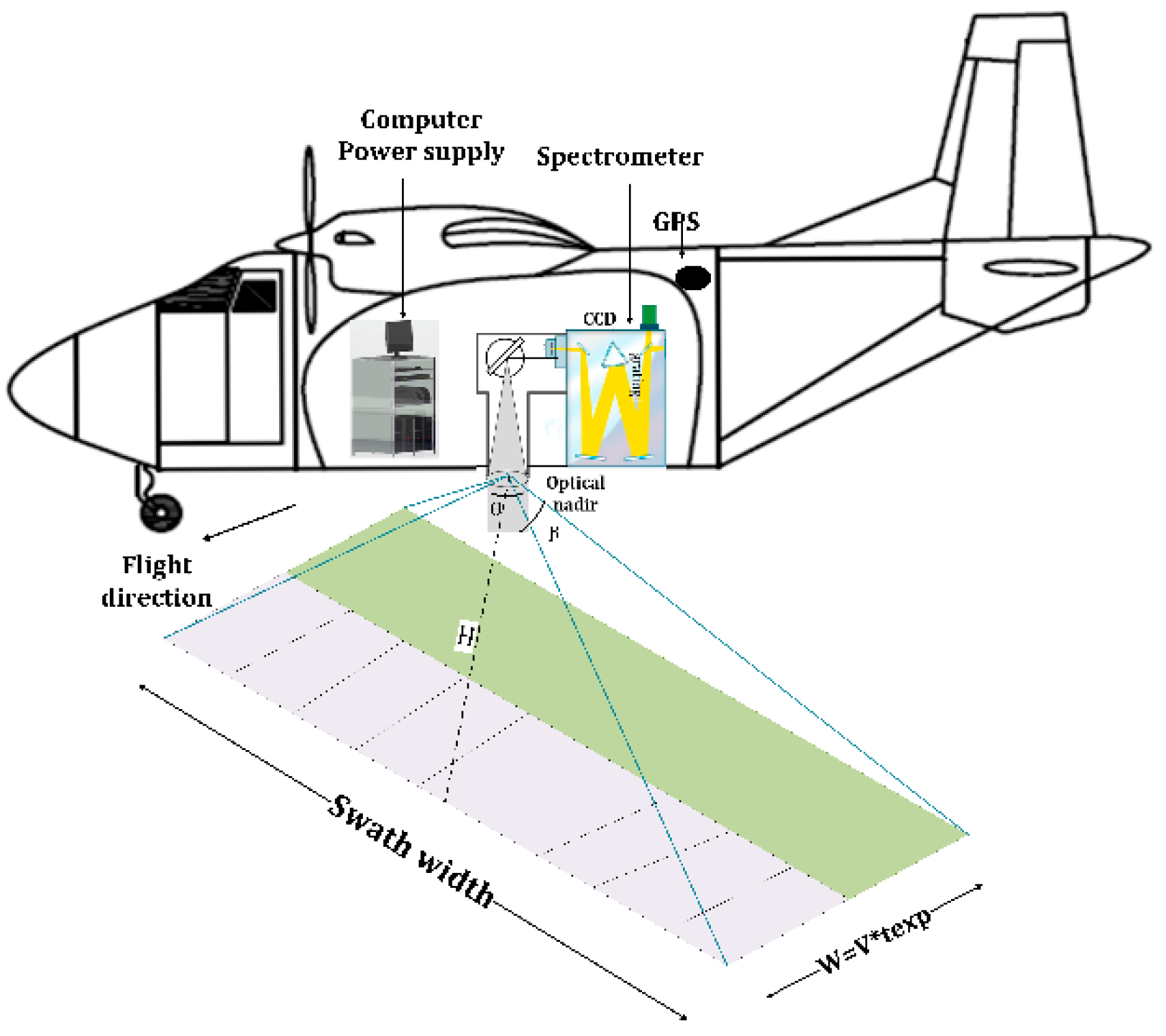
The Air-IRSS developed by the AIOFM-CAS is shown in Figure 1. It comprises three parts: a spectra acquisition unit, a data processing unit, and a GPS. The spectra acquisition unit includes a telescope that collects sunlight at nadir, a fiber, and a spectrometer (Andor 303i). The instantaneous field of view (IFOV) of the Air-IRSS across and along the flight track is 1.16° (θ) × 0.02° (β). At 3 km flight altitude and 180 km/h ground speed, the co-added ground sizes cross, and along the flight track is 62.80 m × 500 m within an exposure time of 1 s. Light is transmitted into the spectrometer by the fiber. The most important component is the high-performance grating spectrometer with a focal length of F = 303 mm, and an f-number of 4. The spectrometer works in the Short Wave Infrared (SWIR) range from 1550 nm to 1650 nm, with a spectral resolution of 0.45 nm. The spectrometer includes an Andor iDus depth-cooled InGaAs 1 × 1024 array detector with a compact design and a dedicated deep thermoelectric cooler that can maintain a minimum temperature of −90℃. The spectra are recorded in the computer and analyzed using the WFM-DOAS algorithm to obtain column concentrations. The distribution of the target gas is then derived in conjunction with the GPS information, which includes geographic information and the speed of the airplane.
A special light source Kr lamp was used to calibrate the slit function of the Air-IRSS. Once the slit function was determined, no further adjustment of the full width at half maximum (FWHM) was required, and the slit function was applied to subsequent data processing.
2.2. Retrieval Algorithm
The WFM-DOAS retrieval algorithm considers absorption cross-section changes due to altitude dependent effects of temperature and pressure, and has been successfully applied to observations in the infrared band [26]; this was discussed in detail by Krings et al. [35]. Furthermore, the WFM-DOAS was further developed specifically to retrieve CO2 from space using SCIAMACHY NIR spectral measurements [37,38,39]. The WFM-DOAS retrieval algorithm is based on a least squares fit of the measured spectra to the modelled spectra, providing the target gas column concentration. As shown in Equation (1), the logarithm of the normalized measured spectrum is the sum of the logarithm of the model radiance, its first derivative, a quadratic polynomial, and the error term.
where and refer to the measured spectrum and modelled radiance at wavelength λ, respectively. is a low order polynomial with free fit parameters denoted as a and is an error term. The low order polynomial is used to account for spectrally smoothly varying parameters that are not explicitly modelled or not well enough known. These parameters, for example, include the Air-IRSS absolute radiometric calibration function, aerosol scattering and absorption parameters, and the surface spectral reflectance. The error term accounts for all wavelength dependent differences between the measurement and the model that cannot be modelled or cannot be modelled without approximations (e.g., aerosol effects). In an ideal case, the error term is identical to the instrument’s detector noise; refers to the reference value of the j-th relevant atmospheric absorber. For CO2 retrieval in this study, the interfering H2O, CH4, and temperature (Temp) were considered. Therefore, j = CO2, H2O, CH4, and Temp. is the target parameter to be retrieved, and for each exists a corresponding . The column weighting functions (CWF) denote the derivatives of radiance with respect to fit parameter . They are computed by adding up all relevant atmospheric layer weighting function as Equation (2).
where zlow and zup represent the lower and upper limits of the relevant atmospheric layers. The layer weighting function can be calculated by the radiance change due to the change of parameter c at altitude z times the quadrature weight . The quadrature weight dependents on the geometrical thickness of the layers of the model atmosphere. Although many atmospheric layers exist, the WFM-DOAS retrieval algorithm does not resolve different altitude levels but shifts the mean profile as a whole. The results of the algorithm are height-averaged increased or decreased profile scaling factors (PSF) or a profile shift (in case of temperature).
3. Retrieval Implementation
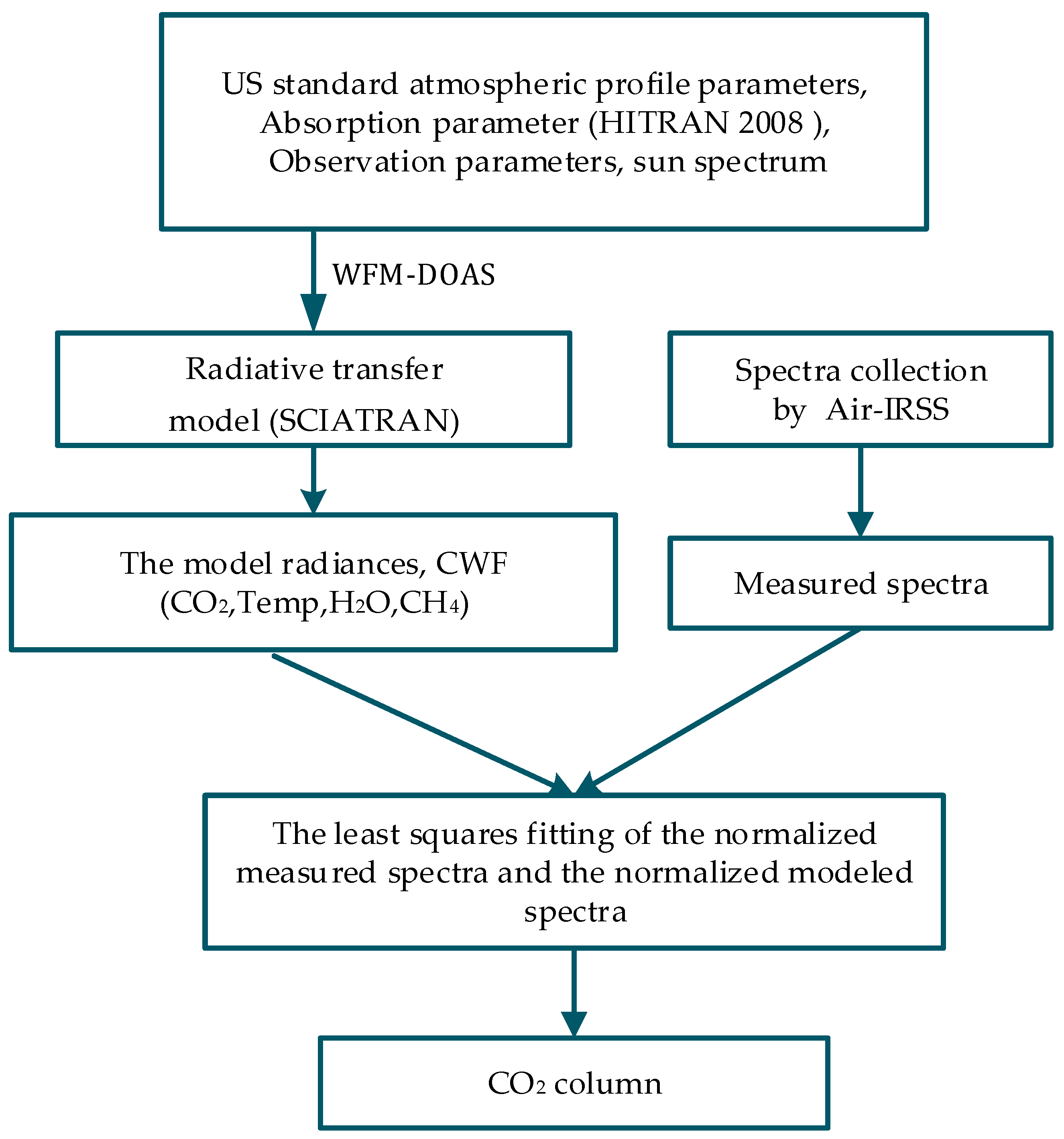
The WFM-DOAS algorithm implementation process is presented in Figure 2. Briefly, the spectra is first recorded by the Air-IRSS instrument via a convolution of the incident radiation with the slit function. The spectra are then passed into the nonlinear least squares spectral fitting subroutine that iteratively generates forward-modelled spectra until the best fit to the measured spectrum is achieved. In on-ground observation mode, the Air-IRSS takes zenith measurements by pointing zenith telescopes directly into the sky. The solar spectra outside the top of the atmosphere is used to normalize the measured spectra. The WFM-DOAS fitting results are the CO2 total column along the total atmosphere. In on-board observation mode, the Air-IRSS takes nadir measurements by pointing telescopes directly into the ground. The zenith spectra recorded above the aircraft is taken as the reference to normalize the measured spectra. The WFM-DOAS fitting results are the CO2 columns below the aircraft. The on-board observations can be used to derive CO2 regional distribution.
3.1. Selection of Retrieval Band
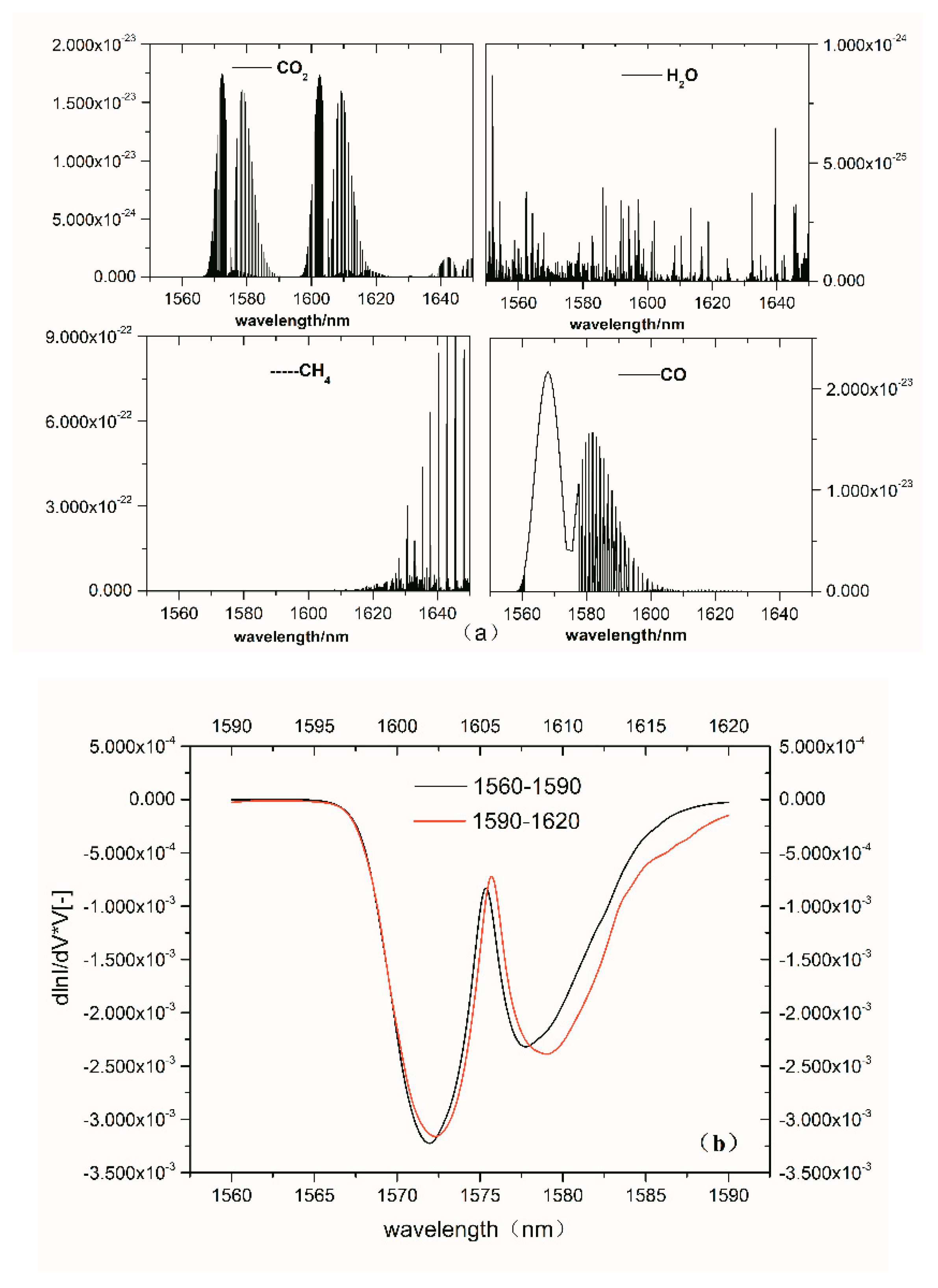
The Air-IRSS works in the bandwidth range from 1550 nm to 1650 nm, which provides two underlying absorption bands for CO2 retrieval (i.e., the 1560–1590 nm band and the 1590–1620 nm band). In both bands, CH4, H2O, and CO are the major interfering gases. The level of interference depends on the interfering absorption intensity times the concentration. Figure 3 shows absorption characteristics of CO2, CH4, H2O, and CO, as well as the CO2 CWF in these two wavelength bands. The CO2 CWF in the 1590–1620 nm band is larger than that in the 1560–1590 nm band. The absorption intensity of CH4 in the 1590–1620 nm band is typically larger than that in the 1560–1590 nm band. The absorption intensities of H2O and CO are comparable in these two wavelength bands. The absorption intensities of CH4, H2O, and CO are lower than that of CO2 by two orders of magnitude. In the atmosphere, the H2O concentration is typically ~30 times larger than that of CO2, and the CH4 and CO concentrations are typically ~200 times lower than that of CO2. Given all of these characteristics, the 1590–1620 nm band was selected for CO2 retrieval, and the H2O and CH4 interference was considered, whereas CO interference was disregarded.
3.2. Retrieval Demonstration
We took spectra obtained at 10:00 local time (LT) on June 18 in Baoding as an example to demonstrate CO2 column retrieval with the Air-IRSS instrument. Both the sun-normalized radiance and its derivatives (i.e., CWF) are computed line-by-line using the radiative transfer model SCIATRAN [40] to simulate the measured spectra. The SCIATRAN was developed by the University of Bremen, and was used extensively to perform radiative transfer modeling in any observation geometry appropriate to measurements of the scattered solar radiation in the Earth’s atmosphere. The model is designed to be used as a forward model in the retrieval of atmospheric constituents from measurements of scattered solar light by satellite, ground-based, or airborne instruments in UV–Vis–NIR spectral region [40]. The input parameters for SCIATRAN simulation are listed in Table 1. Cloud free condition was assumed in the forward model calculation. The HITRAN 2008 spectroscopic database [41] and a solar spectrum by Livingston and Wallace [42] were used. In order to speed up the calculation, the spectra simulations were limited to within the retrieval spectral region between 1590 and 1620 nm. In this study, the absorptions of CO2, CH4, and H2O are included in the calculation. The US standard atmosphere (USSA), with altitude up to 120 km and 53 vertical levels, was assumed in the radiative transfer simulations. Geographical information including solar zenith angles (SZAs), longitude, latitude, and altitude, were directly obtained from the GPS in the Air-IRSS instrument. The a-priori profiles of CO2, CH4, H2O, pressure, and temperature are adopted from USSA but scaled to current concentrations. The instrumental line shape (ILS) of the spectrometer was approximated as a Gaussian function. The aerosol parameterization parameters were adopted from the LOWTRAN database and multiple scattering effects were considered. A pseudo-spherical atmosphere was assumed in radiative transfer calculation and the surface type was assumed to be loam soil.
Figure 4 shows the CWFs of CH4, H2O, CO2, and temperature calculated by SCIATRAN. These CWFs were taken as the reference spectra in WFM-DOAS fitting demonstration in Figure 5. The measured spectrum was well reproduced by the modelled spectrum. The root-mean-square (RMS) of the fitting residuum (the difference between measurement and simulation after the fit) was 0.803%. The fitted CO2 profile scaling factor (PSF) was 0.315 +/− 0.015, which indicates that the retrieved CO2 column below the airplane is 0.3146 times that of the a priori USSA column. The a priori CO2 column used for the SCIATRAN model was 8.188 × 10²¹ molec cm−2; thus, the retrieved CO2 column was 2.58 × 10²¹ +/− 1.27 × 10²⁰ molec cm−2.
4. Sensitivity and Error Estimation
The simulated spectra are significantly affected by numerous observation parameters, such as the atmospheric grid mode, the aerosol type, surface albedo, aircraft altitude, SZA, instrument resolution, and poses in flight. In order to estimate the sensitivity of the retrieved CO2 column to the observation parameters, the retrieval sensitivity was assessed through different radiative transfer simulations. The six observation parameters are listed in Table 2. Each known source of uncertainty is perturbed by several sets of amounts in the SCIATRAN forward model, and the fractional differences in CO2 column for each uncertainty source, relative to the unperturbed case, are computed. These sensitivities are calculated from a spectrum recorded on a typical flight day. The total uncertainty is the sum in quadrature of each individual uncertainty calculated by assuming a realistic perturbation.
4.1. Sensitivity to Vertical Grid Modes
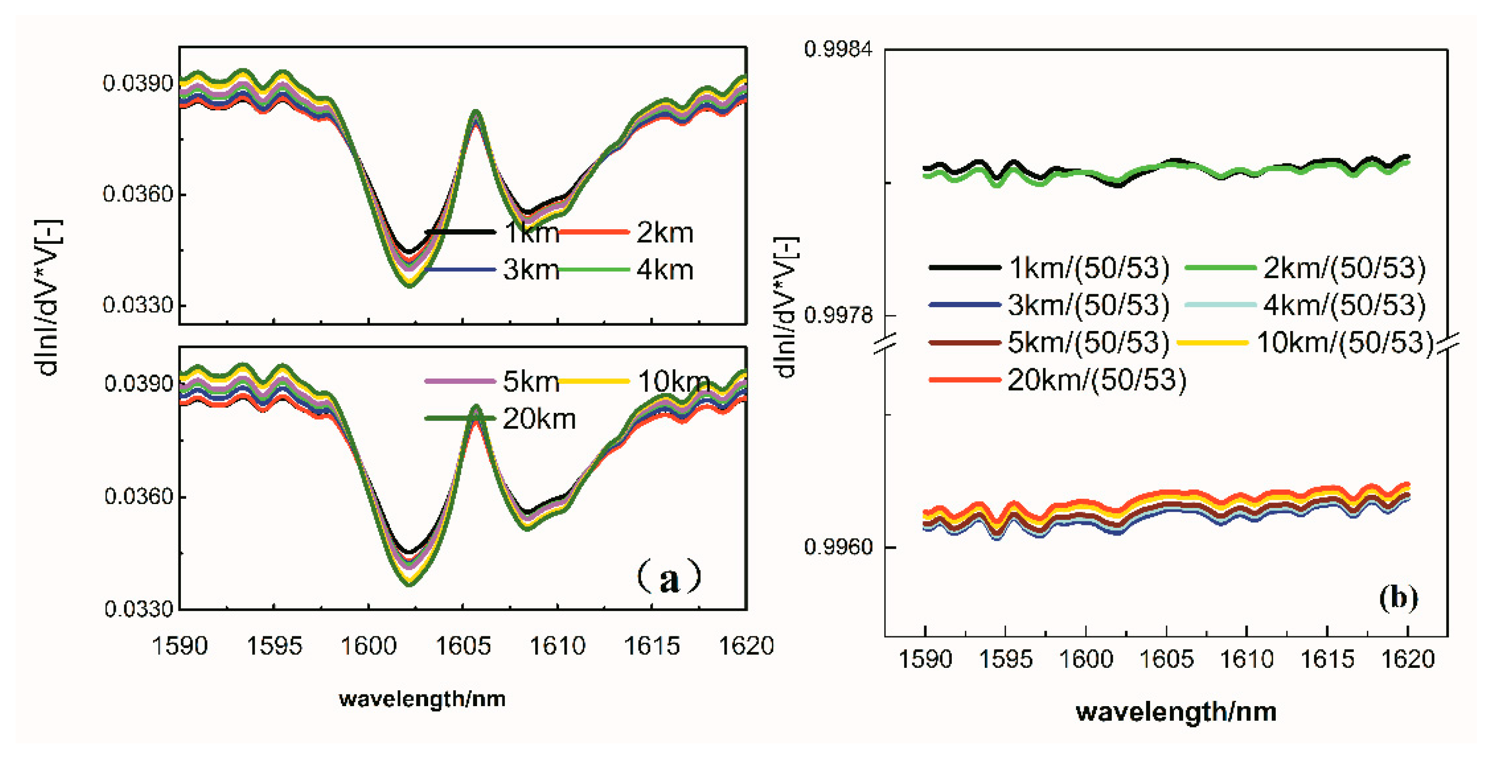
In order to investigate the influence of the vertical layer on retrieval, two kinds of atmospheric grid modes were compared. The first mode separated the total atmosphere into 50 layers. Specifically, the 0–25 km, 25–50 km, and 50–120 km atmosphere were separated into 25, 10, and 14 layers with an interval of 1 km, 2.5 km, and 5 km per layer, respectively. The second mode separated the total atmosphere into 53 layers, where the 0–3 km layer was separated into six layers of 0.5 km per layer, and the separation of the rest of the atmosphere was the same as in the first mode.
The input parameters for simulations with the two modes are listed in Table 3. All parameters used the reference values except the output height, which was perturbed by seven sets of amounts, ranging from 1 km to 20 km. The results, shown in Figure 6, indicate that CO2 absorption under the second grid mode is stronger than that under the first mode (49/53, with a ratio of less than 1, Figure 6b). For both modes, CO2 absorption increases with the output height because with increasing output height, the differential optical path between the measured spectra and the reference spectra increases (Figure 6a). When the output height is less than 3 km, the ratio of the two vertical grid modes is 0.9981. When the output height is greater than 3 km, the ratio of the two vertical grid modes increases with the output height. However, the ratio remains smaller than that at output heights less than 3 km (Figure 6b). Given that the Air-IRSS is designated to work in the flight altitude range of 0–3 km (the second grid mode), the finer grid results in a smaller effect on the retrieval compared with the first one.
4.2. Sensitivity to Aerosol Type
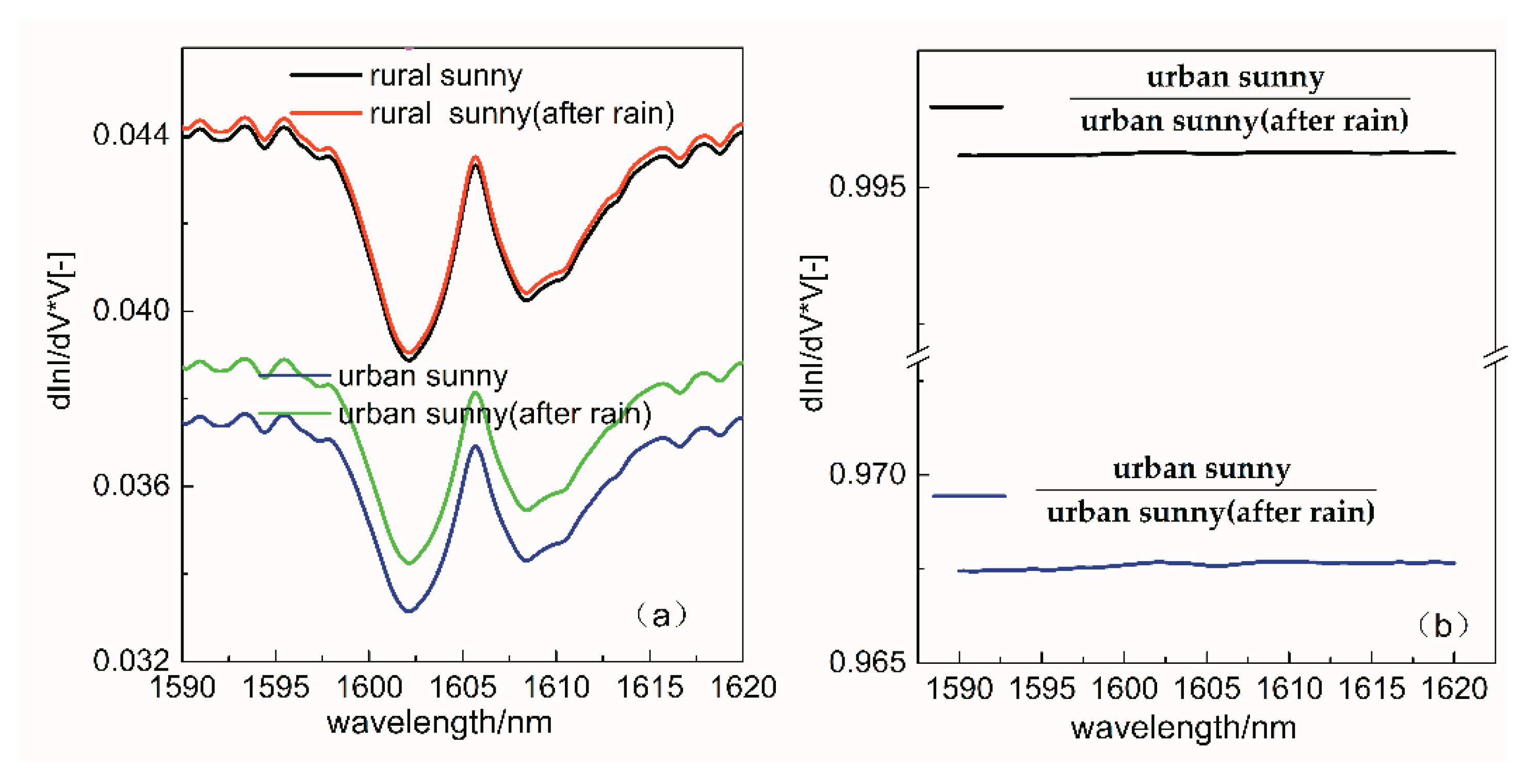
The flight observation crosses two types of areas (i.e., urban and rural areas). Therefore, two different types of aerosols are used for urban and rural areas. Considering the actual weather conditions during airborne measurements, sunny weather was divided into two cases: continuous sunny days and sunny days after rain. The sensitivity of CO2 CWF with respect to four different types of aerosols is shown in Figure 7, and the resulting statistics are listed in Table 4. As shown in Figure 7a, the CO2 CWF for the rural case is larger than that for the urban case. Furthermore, the CO2 CWF in the case of sunny days after rain is larger than continuous sunny days. A smaller CO2 CWF indicates a larger CO2 vertical column. These simulation results are in good agreement with the actual situation, in which the CO2 vertical column in city areas is larger than that in rural areas. CO2 concentration in the case of sunny days after the rain was smaller than that in the case of continuous sunny days, because the atmosphere can be purified by rainwater. The influence of rainwater on the two types of aerosols was also different, i.e., the influence was more significant in the case of city areas than in the case of rural areas, as shown in Figure 7b.
4.3. Sensitivity to Other Parameters
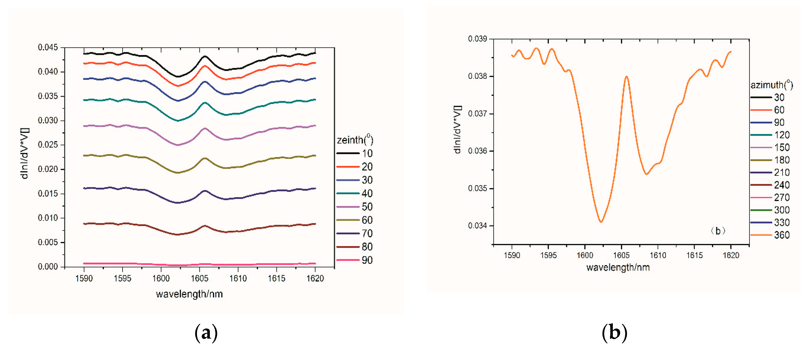
The sensitivity of CO2 CWF to solar zenith angle, azimuth angle, surface albedo, spectral resolution, and output altitude are shown in Figure 8, and the corresponding statistics are listed in Table 5.
SZA
The solar zenith angle, in the range of 0–90°, is the angle between the sun’s rays and the zenith. When the angle is small, photon scattering mainly occurs in the lower troposphere. When the solar zenith angle is larger than 45º, the scattering mainly occurs in the stratosphere. The SZA has a significant influence on the optical path. Investigating the influence of SZA is beneficial in the selection of the reference spectra because the sun’s position changes regularly during the day. In the present study, nine angles were selected: 10°, 20°, 30°, 40°, 50°, 60°, 70°, 80°, and 90°. When the solar zenith angle is greater than 75°, calculation errors will increase due to the limitations of the model. Thus, the flight measurement was conducted within an effective time when the SZA was smaller than 75°. As shown in Figure 8a, the CO2 CWF decreases as the SZA increases and a smaller SZA results in a larger CO2 CWF. Furthermore, the variation of CO2 CWF at low SZA is less sensitive to the variation of SZA than that at high SZA. Therefore, the most optimal time for airborne experiments is at noon.
Azimuth Angle
The azimuth angle, in the range of 0–360°, is the angle between the sun’s rays and Earth’s due north. Figure 8b shows that the CWF did not change with the azimuth angles. Therefore, the influence of the azimuth angle could be ignored in CO2 retrieval with the Air-IRSS spectra.
Surface Albedo
In airborne observation, light is received mainly from surface reflection, and with increasing surface albedo, the light intensity reflected from the surface increases. Therefore, surface albedo is an important parameter to be considered in the present study. In order to study this effect, different surface albedo values were set in the simulation: 0.02, 0.05, 0.1, 0.2, 0.3, 0.4, 0.5, 0.6, 0.7, 0.8, 0.9, and 1.0. As shown in Figure 8c, the CO2 CWF increased with increasing surface albedo. Therefore, the retrieval accuracy could be improved by optimizing the surface albedos for different types of surfaces.
Spectral Resolution
The selection of spectral resolution is related to the absorption line width of the target gas, and the closer the resolution is to the actual absorption structure of the target gas, the more accurate the retrieval results will be. As shown in Figure 8d, fine absorption structures can be observed when the resolution is sufficiently high. As the resolution increased further, the CO2 CWF increased and the fine absorption structures disappeared, resulting in a smooth CO2 absorption peak. The CO2 absorption line was located very near the wavelength range of 1590–1620 nm, and an error in the instrument line shape would be expected to cause an error in the CO2 retrieval. Therefore, the instrument resolution should be optimized for the spectral measurement conditions.
Output Altitude
The optical path changes with the flight altitude. In the simulation, eleven output altitudes of 0.5, 1.0, 2.0, 3.0, 4.0, 5.0, 6.0, 7.0, 8.0, 9.0, and 10 km were selected. As shown in Figure 8e, the CO2 CWF decreases with output height. In addition, the rate of the decrease in the CWF becomes smaller with increasing output height. This result also indicates that CO2 absorption in the low-altitude region is much larger than that in the high-altitude region. When the flight altitude of 3 km is set as the reference altitude, the value of the CWF will obviously change, even with small fluctuations in altitude. In the retrieval process, the grid is refined as an altitude below 3 km to improve the precision.
4.4. Total Error Estimation
In addition to the above uncertainty sources, the uncertainties of a priori profiles of CO2, pressure, and temperature also lead to potential retrieval errors. In order to assess the influence of these factors in the total uncertainty, the following hypothesis was applied: the temperature or pressure a priori profile increases or decreases by 1 K/1 hPa at all altitudes when the a priori profile of CO2 is shifted downward or upward by 1 km. Table 6 lists typical uncertainties that may generally be expected for a retrieval of CO2 total column using the WFM-DOAS. The total uncertainty estimated for the retrieval of the CO2 column was found to be 1.26% for airborne WFM-DOAS over a large region, and 0.30% for a fixed point, such as power points or factories, which shows that the parameters of flight experiments over the North China Plain can meet the accuracy requirements of data retrieval.
5. Application and Discussion
5.1. Comparison with GOSAT
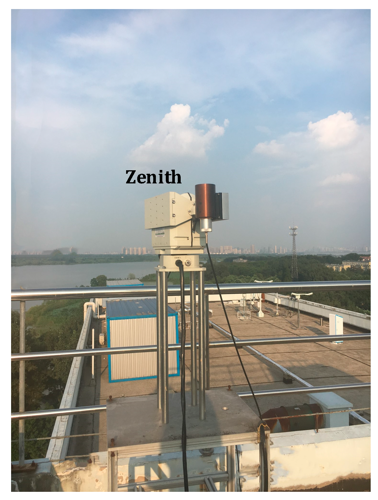
In order to investigate the instrument’s performance under vibration-free static conditions, the on-ground Air-IRSS results were compared with the GOSAT observations. The Air-IRSS, shown in Figure 9, was deployed on the roof of a six-story building at the AIOFM-CAS campus (117.158°E, 31.908°N). The observation site is adjacent to the Shu Shan Lake that covers an area of 207.5 km2. This area is prevailed by southeast winds in summer and northwest winds in winter. The observation site is adjacent to the Shu Shan Lake, which covers an area of 207.5 km2. In this area southeast winds prevail in the summer, and northwest winds prevail in the winter. The regional landscape is mostly flat with a few hills. Downtown of Hefei is located in the southeast of this site and is densely populated with seven million people. In other directions, the site is surrounded by wetlands or cultivated lands. The relevant anthropogenic emissions mainly originate from the city, and natural emissions originate from cultivated lands or wetlands. The scattered light zenith radiance measurements (measurements of the down-welling diffuse radiance) were performed by pointing the Air-IRSS zenith telescopes directly into the sky. The spectra were collected under clear sky conditions with a single readout exposure time of 4 s and an average times of 5.
The selection of the coincidence criterion is of great significance, and generally the stricter the criterion, the better the satellite validation. The best choice would be the time-scale; the spatial coverage of Air-IRSS observations is the same as that of the satellite data. However, in reality, a compromise criterion needs to be used to balance the accuracy and the number of the valid data. Since GOSAT does not target the Hefei site, the strict criteria (e.g., 1°) would result in very sparse valid data. A relatively relaxed criterion can produce more valid data but does not influence the validation considerably, because at the GOSAT overpass time (13:00 ± 00:15 LT), SZA is very small and the surrounding emissions have a small influence on the observations. In this study, a relatively relaxed criterion was used; that is, the mean of the GOSAT data was selected within the 5° latitude and longitude rectangular area around the Hefei site, and the mean of Air-IRSS data was selected within 30 min of the GOSAT overpass time. This coincidence criterion is a balance between the accuracy and the number of valid data.
The time series and correlation plot of CO2 columns obtained by Air-IRSS and GOSAT are shown in Figure 10. Generally, the two instruments are in good agreement. The Air-IRSS observations can reproduce the variations observed by GOSAT well with a correlation coefficient (R2) of 0.72. The CO2 total columns of Air-IRSS and GOAST are on average of 8.63 × 10²¹ molec cm−2 and 8.89 × 10²¹ molec cm−2, respectively. Average differences between Air-IRSS and GOSAT data (Air-IRSS minus GOSAT) were −0.26 × 10²¹ molec cm−2 (−2.90%). This discrepancy is most likely due to the usage of a relatively relaxed criterion, which results in a relatively larger inhomogeneity (Figure 11). Regionally higher CO2 level over emission sources, such as densely popularized area or industrialized area, could aggravate the inhomogeneity within the selected GOSAT coverage, and thus aggravate the difference. Meanwhile, the mismatch of temporal resolution (±0.5 h) could also cause difference between the Air-IRSS and GOSAT.
5.2. Airborne Field Campaign
5.2.1. Field Campaign Description
On June 16 and 18, 2016, an 8-h airborne field campaign was conducted at Luancheng Airport (114.4°E, 37.8°N) in Hebei Province (including four cities of Xing-tai, Baoding, Henshui, and Shijiazhuang). The Air-IRSS was deployed on a Y-5 aircraft with a nadir telescope. The spectra were collected during the flight with an integration time of 1 s and an average number of 10. The latitude, longitude, and altitude data were recorded by a GPS device (data acquisition speed of 1 HZ) on the aircraft. The flight altitudes were from 200 to 3000 m and the flight speed ranged from 140 to 200 km/h. Two groups of flight experiments were conducted: one on June 16, 13:30–16:10, and the other on June 18, 08:20–13:20 local time. The fight trajectories are shown in Figure 12. On June 16, starting from Luancheng Airport, the aircraft initially passed over the hilly Xing-tai Mountain Area and then returned to the airport over Xing-tai City. On June 18, the aircraft departed from Luancheng Airport and passed over Baoding, Hengshui, and Shijiazhuang, finally returning to Luancheng Airport.
5.2.2. Results and Discussion
In order to minimize the impacts of significant weather events or instrument problems, we established a specific filter criterion to remove outliers by setting certain thresholds for measurement intensity, SNR, and fitting residuals. Measurements satisfying the following criteria were classified as valid and were subsequently used in the analysis.
- (1)
- Spectra recorded with insufficient incident signals were discarded to ensure adequate SNR, and spectra recorded with excessive incident signals were discarded because of non-linearity in the detector. These criteria ensured that the SNR would be larger than 500 and the detector would be less than 70% saturated.
- (2)
- Auxiliary data, such as GPS information, solar intensity, and meteorological data that were not recorded synchronously with the measurement, were eliminated.
- (3)
- The observed scene had to be nearly cloud-free and not seriously affected by smog or unknown opaque objects. Spectra recorded with a solar intensity variation (SIV) of more than 10% were not used in this study, where the SIV was defined as the ratio of the standard deviation to the average of the sun intensities within the duration of a spectrum.
- (4)
- The RMS of the residual difference (relative difference between measured and calculated spectra after the fit) has to be less than 2%.
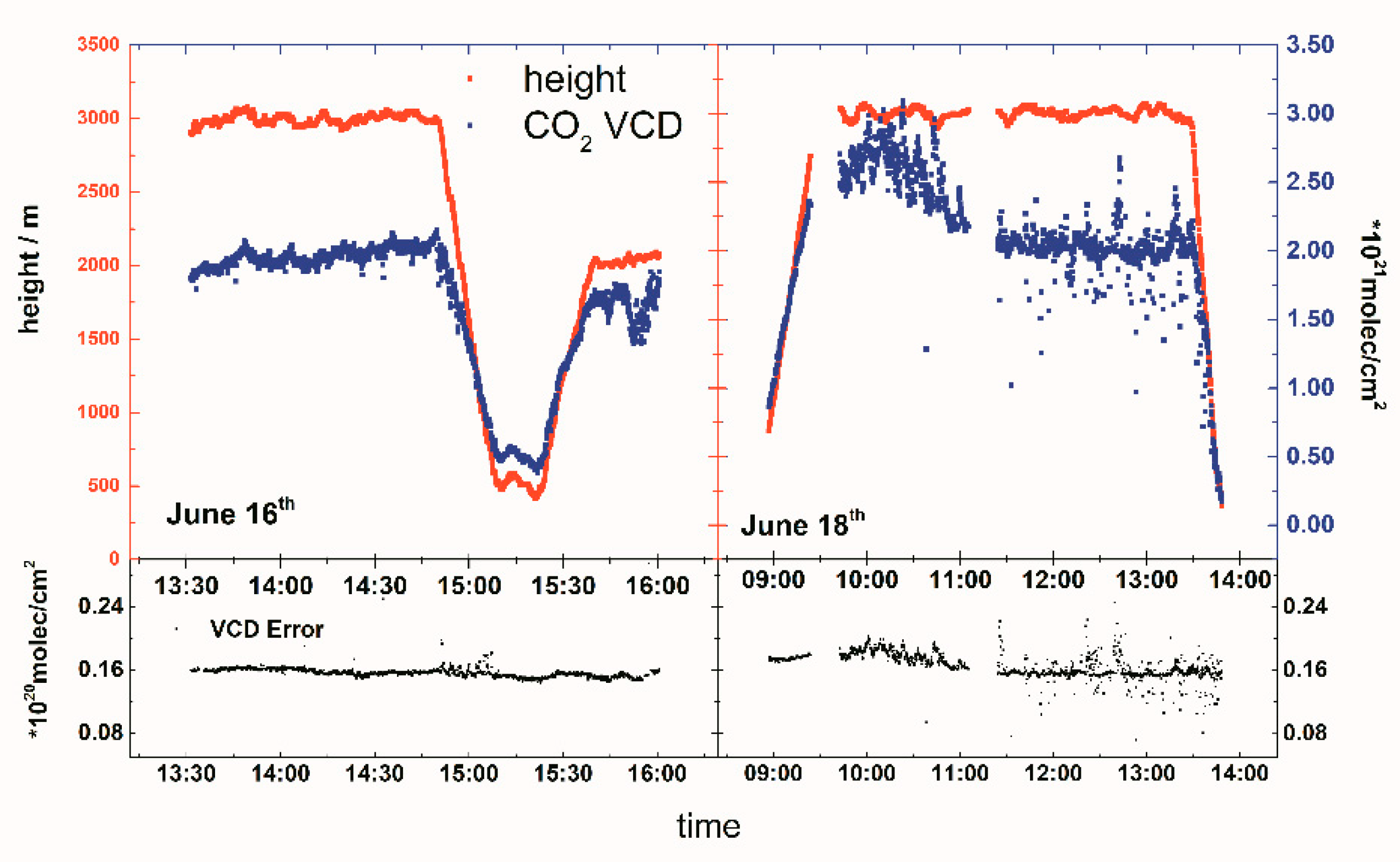
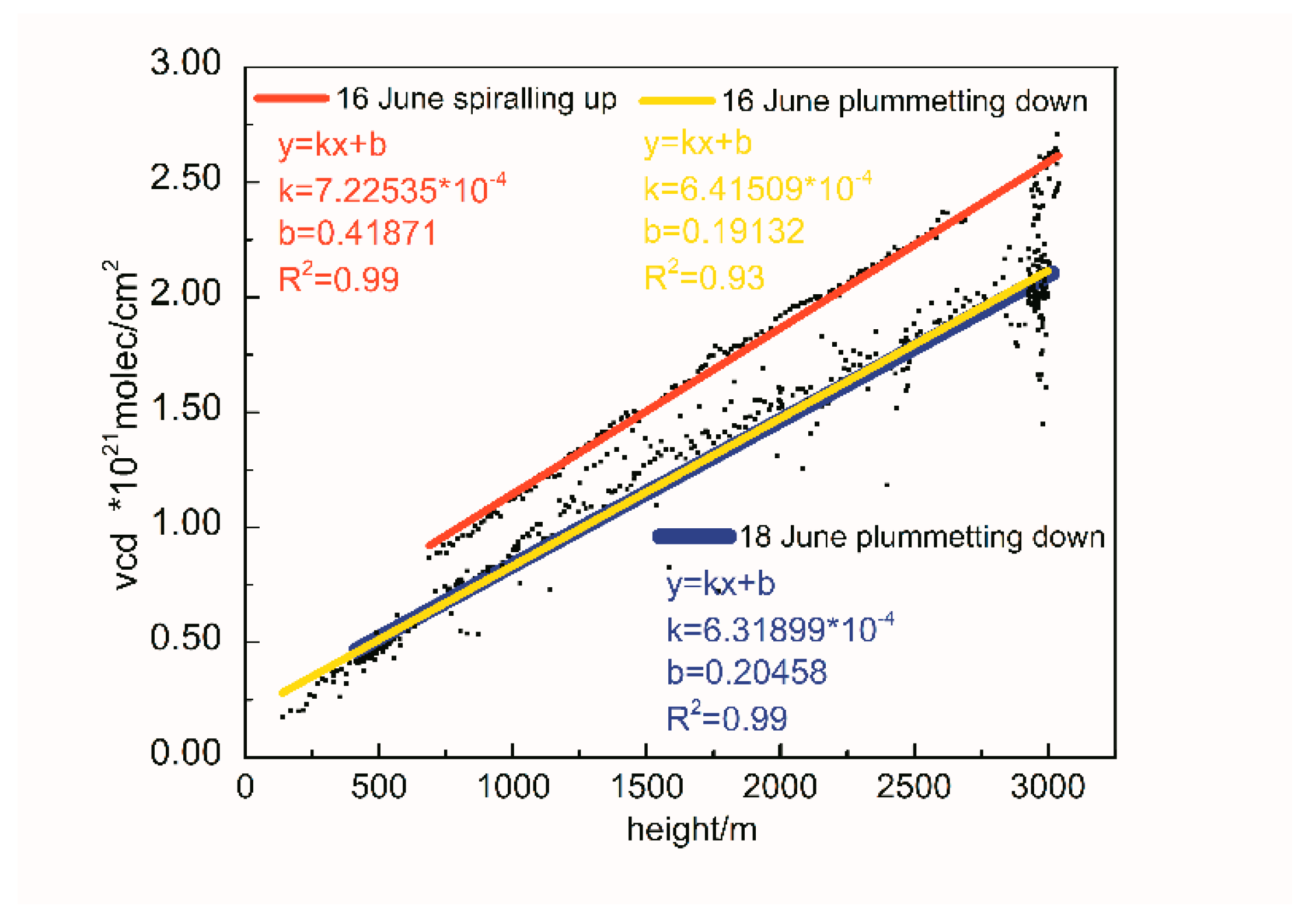
Figure 13 shows temporal variations in the retrieved CO2 column along with the flight altitude. The aircraft flew smoothly at 3 km in the period of 13:32–15:35 on June 16 and 09:36–14:35 on June 18. In contrast, it circled up and down between 500 m and 3000 m in the rest of the time. The CO2 column varied in the range of 0.50–3.00 × 10²¹ molec cm−2, and the RES of the CO2 column ranged from 0.60% to 1.20%. On June 18, the CO2 column at 09:36–11:00 was higher than that at 11:00–14:35 by approximately (0.30–0.80) × 1021 molec cm−2, even though the flight altitude was not changed. This is because the emissions are not consistent in different areas. Figure 14 shows the linear fit between the CO2 column and the altitude. The data were only collected during spiral up and plummet down stages. The spiral up data were obtained on June 16 (at an average surface altitude of 160 m) and the plummet down data were obtained on June 16 (at an average surface altitude of 60 m) and June 18 (an average surface altitude of 60 m). The results show that the CO2 column below the aircraft was highly correlated with aircraft altitude and the higher the altitude, the larger the CO2 columns. The CO2 columns at the spiral up stage were approximately (1.90–2.00) × 1020 molec cm−2 higher than those at the plummet down stage, mainly because the surface topography within the plummet down stage was 100–110 m higher than that of the spiral up stage.
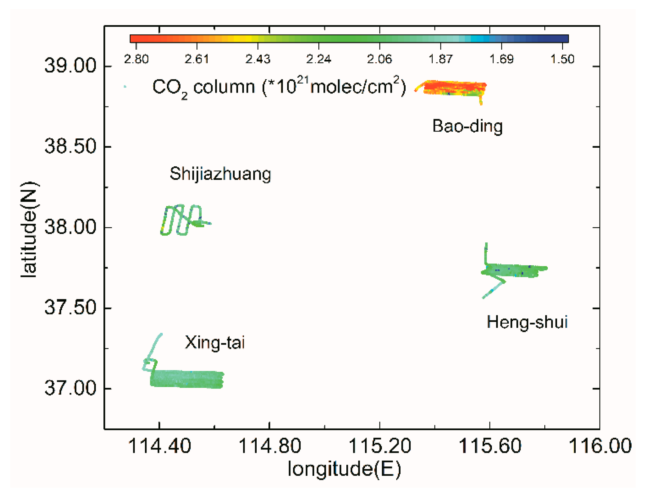
As shown in Figure 15, the regional distribution of CO2 was obtained with the GPS information. The CO2 column ranged from 2.00 × 10²¹ molec cm-2 to 2.50 × 10²¹ molec cm−2 in the three cities of Xing-tai, Hengshui, and Shijiazhuang, with a uniform distribution. The CO2 column was high only at Baoding, at approximately (2.50–3.00) × 1021 molec cm−2; the CO2 column in the northern part of Baoding city was higher than that in the south. The CO2 column in Xing-tai city was approximately (2.50–3.00) × 1020 molec cm-2 higher than that in the Xingtai Mountainous Area. The column concentration is higher in the northern part of Xing-tai city than in the south by approximately (1.00–1.50) × 1020 molec cm−2. The values in the eastern and western areas were higher than those in the city center, which was approximately (1.00–1.40) × 1020 molec cm−2.
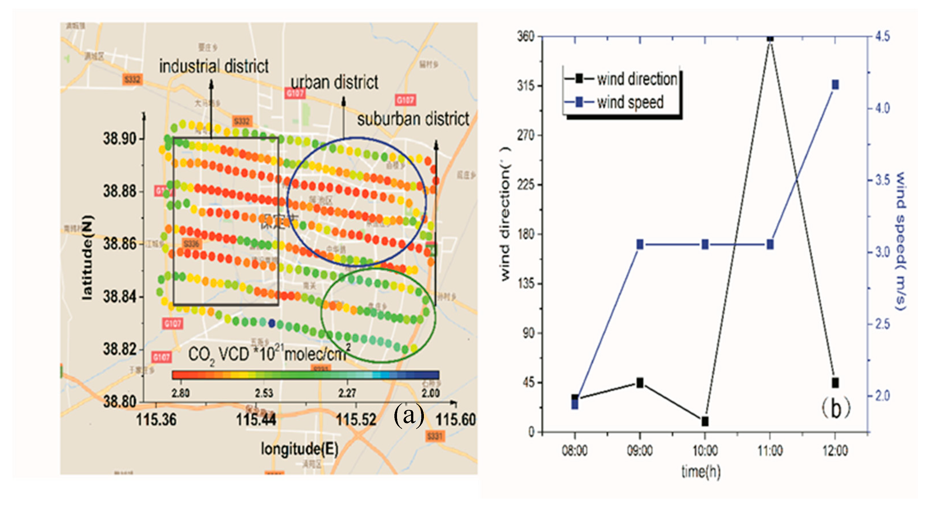
In addition, a detailed analysis of Baoding was conducted because the CO2 column in this area is the highest among the four cities. As shown in Figure 16a (sourced from Google Maps), several major CO2 emissions sources are distributed in the flight area. Three functional zonings of Baoding can be identified: industrial district, urban district, and suburban district. There are several large emission sources in the industrial district, including large thermal power plants, paper mills, breweries, and cigarette factories. The flight time in Baoding was from 9:00 to 11:20 on June 18. The wind speed and wind direction are shown in Figure 16b. A northeast wind prevailed from 9:00 to 10:00, and a north wind prevailed from 10:00 to 11:20, with a steady wind speed at 3.0 m/s. The Figure 16a shows that the CO2 column was high around the CO2 sources and along the wind direction. Since a large number of emission sources are distributed north of the flight area, the CO2 column in the northern part of the flight area was higher than that in the south.
6. Conclusions
This study presented a self-made airborne infrared remote sensing spectrometer (Air-IRSS) designated to determine the regional distribution of CO2. It measured CO2 in the spectral range between 1590 and 1620 nm at a spectral resolution of 0.45 nm and an exposure time of 1 s. The Air-IRSS was operated onboard an aircraft at a height of 3 km with a velocity of 180 km/h. The instantaneous field of view (IFOV) of the Air-IRSS is 1.16° (across the flight track) × 0.02° (along the flight track), which corresponds to a ground size of 50.00 m × 62.80 m. The weighting function modified differential optical absorption spectroscopy (WFM-DOAS) technique was used to analyze the measured spectra.
In order to estimate the sensitivity of the retrieved CO2 columns to the observation parameters, retrieval sensitivity with respect to different radiative transfer simulations have been performed. The total uncertainty estimated for the retrieval of the CO2 column was found to be 1.26% for airborne measurements over a large region, and 0.30% for a fixed point, such as power points or factories. In order to investigate the instrument’s performance under vibration-free static conditions, the on-ground Air-IRSS results were compared with the GOSAT observations. The on-ground Air-IRSS observations can reproduce the variations observed by GOSAT well, with a correlation coefficient (r) of 0.72. Finally, we conducted an airborne field campaign to determine the regional distribution of CO2 in the North China Plain. The regional distribution of CO2 over four cities of Xing-tai, Hengshui, and Shijiazhuang, and Baoding were obtained with the GPS information. The CO2 columns of these four cities ranged from 2.00 × 10²¹ molec cm−2 to 3.00 × 10²¹ molec cm−2. The CO2 vertical distributions were almost uniform below a height of 3 km in the area without CO2 emission sources, and the highest values were found in Baoding City due to the contributions of the emission sources, such as power plants and factories.
Author Contributions
P.X., J.X., and A.L. conceived, designed the experiments. R.W. and J.X. performed the experiments. R.W. analyzed the data. R.W. wrote the paper. P.X., J.X., and Y.S. improved the paper.
Funding
This work was supported by the Key Program of the National Natural Science Foundation of China (No: 41530644), the Young Scientists Fund of the National Natural Science Foundation of China(No: 41405033), the National High Technology Research and Development Program of China (No: 2014AA06A508, No. 2016YFC0200800), the National key research and development program (NO: 2017YFC0209902), and the National Science Foundation of China (No. 41605018, No.41877309).
Conflicts of Interest
The authors declare no conflict of interest.
References
- Buchwitz, M.; de Beek, R.; Burrows, J.P.; Bovensmann, H.; Warneke, T.; Notholt, J.; Meirink, J.F.; Goede, A.P.H.; Bergamaschi, P.; Korner, S.; et al. Atmospheric methane and carbon dioxide from SCIAMACHY satellite data: Initial comparison with chemistry and transport models. Atmos. Chem. Phys. 2005, 5, 941–962. [Google Scholar] [CrossRef]
- Wunch, D.; Toon, G.C.; Wennberg, P.O.; Wofsy, S.C.; Stephens, B.B.; Fischer, M.L.; Uchino, O.; Abshire, J.B.; Bernath, P.; Biraud, S.C.; et al. Calibration of the Total Carbon Column Observing Network using aircraft profile data. Atmos. Meas. Tech. 2010, 3, 1351–1362. [Google Scholar] [CrossRef] [Green Version]
- Wunch, D.; Toon, G.C.; Blavier, J.F.; Washenfelder, R.A.; Notholt, J.; Connor, B.J.; Griffith, D.W.; Sherlock, V.; Wennberg, P.O. The total carbon column observing network. Philos. Trans. A Math. Phys. Eng. Sci. 2011, 369, 2087–2112. [Google Scholar] [CrossRef] [PubMed]
- Barros, V.R.; Field, C.B.; Dokken, D.J. IPCC: Climate Change 2014; Cambridge University Press: Cambridge, UK, 2014; p. 688. [Google Scholar]
- Paul, D.; Chen, H.; Been, H.A.; Kivi, R.; Meijer, H.A.J. Radiocarbon analysis of stratospheric CO2 retrieved from AirCore sampling. Atmos. Meas. Tech. 2016, 9, 4997–5006. [Google Scholar] [CrossRef]
- Stephens, B.B.; Gurney, K.R.; Tans, P.P.; Sweeney, C.; Peters, W.; Bruhwiler, L.; Ciais, P.; Ramonet, M.; Bousquet, P.; Nakazawa, T.; et al. Weak northern and strong tropical land carbon uptake from vertical profiles of atmospheric CO2. Science 2007, 316, 1732–1735. [Google Scholar] [CrossRef] [PubMed]
- Chevallier, F.; Bréon, F.-M.; Rayner, P.J. Contribution of the Orbiting Carbon Observatory to the estimation of CO2 sources and sinks: Theoretical study in a variational data assimilation framework. J. Geophys. Res. 2007, 112. [Google Scholar] [CrossRef]
- Miller, C.E.; Crisp, D.; DeCola, P.L.; Olsen, S.C.; Randerson, J.T.; Michalak, A.M.; Alkhaled, A.; Rayner, P.; Jacob, D.J.; Suntharalingam, P.; et al. Precision requirements for space-based data XCO2 data. J. Geophys. Res. Atmos. 2007, 112. [Google Scholar] [CrossRef]
- Gayraud, N.; Kornaszewski, L.W.; Stone, J.M.; Knight, J.C.; Reid, D.T.; Hand, D.P.; MacPherson, W.N. Mid-infrared gas sensing using a photonic bandgap fiber. Appl. Opt. 2008, 47, 1269–1277. [Google Scholar] [CrossRef] [PubMed]
- Kim, K.J.; Chong, X.Y.; Kreider, P.B.; Ma, G.H.; Ohodnicki, P.R.; Baltrus, J.P.; Wang, A.X.; Chang, C.H. Plasmonics-enhanced metal-organic framework nanoporous films for highly sensitive near-infrared absorption. J. Mater. Chem. C 2015, 3, 2763–2767. [Google Scholar] [CrossRef]
- Lai, W.C.; Chakravarty, S.; Wang, X.; Lin, C.; Chen, R.T. On-chip methane sensing by near-IR absorption signatures in a photonic crystal slot waveguide. Opt. Lett. 2011, 36, 984–986. [Google Scholar] [CrossRef] [PubMed]
- Ying, H.; Yujun, Z.; Liming, W.; Kun, Y.; Xiaomin, S.; Zhenmin, L. Laser technology for CO2 and H2O on-line detection in large-scale region. Chin. J. Lasers 2014, 42, 0115003-1. [Google Scholar] [CrossRef]
- Chan, K.L.; Ning, Z.; Westerdahl, D.; Wong, K.C.; Sun, Y.W.; Hartl, A.; Wenig, M.O. Dispersive infrared spectroscopy measurements of atmospheric CO2 using a Fabry-Perot interferometer sensor. Sci. Total Environ. 2014, 472, 27–35. [Google Scholar] [CrossRef] [PubMed]
- Oh, Y.S.; Kenea, S.T.; Goo, T.Y.; Chung, K.S.; Rhee, J.S.; Ou, M.L.; Byun, Y.H.; Wennberg, P.O.; Kiel, M.; DiGangi, J.P.; et al. Characteristics of greenhouse gas concentrations derived from ground-based FTS spectra at Anmyeondo, South Korea. Atmos. Meas. Tech. 2018, 11, 2361–2374. [Google Scholar] [CrossRef] [Green Version]
- Kiel, M.; Wunch, D.; Wennberg, P.O.; Toon, G.C.; Hase, F.; Blumenstock, T. Improved retrieval of gas abundances from near-infrared solar FTIR spectra measured at the Karlsruhe TCCON station. Atmos. Meas. Tech. 2016, 9, 669–682. [Google Scholar] [CrossRef] [Green Version]
- Velazco, V.A.; Morino, I.; Uchino, O.; Hori, A.; Kiel, M.; Bukosa, B.; Deutscher, N.M.; Sakai, T.; Nagai, T.; Bagtasa, G.; et al. TCCON Philippines: First Measurement Results, Satellite Data and Model Comparisons in Southeast Asia. Remote Sens. 2017, 9, 1228. [Google Scholar] [CrossRef]
- Morino, I.; Uchino, O.; Inoue, M.; Yoshida, Y.; Yokota, T.; Wennberg, P.O.; Toon, G.C.; Wunch, D.; Roehl, C.M.; Notholt, J.; et al. Preliminary validation of column-averaged volume mixing ratios of carbon dioxide and methane retrieved from GOSAT short-wavelength infrared spectra. Atmos. Meas. Tech. 2011, 4, 1061–1076. [Google Scholar] [CrossRef] [Green Version]
- Frankenberg, C.; Pollock, R.; Lee, R.A.M.; Rosenberg, R.; Blavier, J.F.; Crisp, D.; O’Dell, C.W.; Osterman, G.B.; Roehl, C.; Wennberg, P.O.; et al. The Orbiting Carbon Observatory (OCO-2): Spectrometer performance evaluation using pre-launch direct sun measurements. Atmos. Meas. Tech. 2015, 8, 301–313. [Google Scholar] [CrossRef]
- Schneising, O.; Buchwitz, M.; Burrows, J.P.; Bovensmann, H.; Bergamaschi, P.; Peters, W. Three years of greenhouse gas column-averaged dry air mole fractions retrieved from satellite—Part 2: Methane. Atmos. Chem. Phys. 2009, 9, 443–465. [Google Scholar] [CrossRef]
- Ying, H.; Yujun, Z.; Liming, W.; Kun, Y.; Xiaomin, S.; Zhenmin, L. A Comparison of the Atmospheric CO2 Concentrations Obtained by an Inverse Modeling System and Passenger Aircraft Based Measurement. Atmosphere 2016, 26, 387–400. [Google Scholar]
- Machida, T.; Matsueda, H.; Sawa, Y.; Nakagawa, Y.; Hirotani, K.; Kondo, N.; Goto, K.; Nakazawa, T.; Ishikawa, K.; Ogawa, T. Worldwide Measurements of Atmospheric CO2 and Other Trace Gas Species Using Commercial Airlines. J. Atmos. Ocean. Technol. 2008, 25, 1744–1754. [Google Scholar] [CrossRef]
- Gerilowski, K.; Tretner, A.; Krings, T.; Buchwitz, M.; Bertagnolio, P.P.; Belemezov, F.; Erzinger, J.; Burrows, J.P.; Bovensmann, H. MAMAP—A new spectrometer system for column-averaged methane and carbon dioxide observations from aircraft: Instrument description and performance analysis. Atmos. Meas. Tech. 2011, 4, 215–243. [Google Scholar] [CrossRef]
- Houweling, S.; Hartmann, W.; Aben, I.; Schrijver, H.; Skidmore, J.; Roelofs, G.J.; Breon, F.M. Evidence of systematic errors in SCIAMACHY-observed CO2 due to aerosols. Atmos. Chem. Phys. 2005, 5, 3003–3013. [Google Scholar] [CrossRef]
- Platt, U. Dry Deposition of SO2. Atmos. Environ. 1978, 12, 363–367. [Google Scholar] [CrossRef]
- Reuter, M.; Bovensmann, H.; Buchwitz, M.; Burrows, J.P.; Connor, B.J.; Deutscher, N.M.; Griffith, D.W.T.; Heymann, J.; Keppel-Aleks, G.; Messerschmidt, J.; et al. Retrieval of atmospheric CO2 with enhanced accuracy and precision from SCIAMACHY: Validation with FTS measurements and comparison with model results. J. Geophys. Res.-Atmos. 2011, 116. [Google Scholar] [CrossRef]
- Buchwitz, M.; Rozanov, V.V.; Burrows, J.P. A near-infrared optimized DOAS method for the fast global retrieval of atmospheric CH4, CO, CO2, H2O, and N2O total column amounts from SCIAMACHY Envisat-1 nadir radiances. J. Geophys. Res.-Atmos. 2000, 105, 15231–15245. [Google Scholar] [CrossRef]
- Chan, K.L.; Wiegner, M.; Wenig, M.; Pohler, D. Observations of tropospheric aerosols and NO2 in Hong Kong over 5 years using ground based MAX-DOAS. Sci. Total Environ. 2018, 619, 1545–1556. [Google Scholar] [CrossRef] [PubMed]
- Chan, K.L.; Hartl, A.; Lam, Y.F.; Xie, P.H.; Liu, W.Q.; Cheung, H.M.; Lampel, J.; Pohler, D.; Li, A.; Xu, J.; et al. Observations of tropospheric NO2 using ground based MAX-DOAS and OMI measurements during the Shanghai World Expo 2010. Atmos. Environ. 2015, 119, 45–58. [Google Scholar] [CrossRef]
- Wu, F.C.; Xie, P.H.; Li, A.; Mou, F.S.; Chen, H.; Zhu, Y.; Zhu, T.; Liu, J.G.; Liu, W.Q. Investigations of temporal and spatial distribution of precursors SO2 and NO2 vertical columns in the North China Plain using mobile DOAS. Atmos. Chem. Phys. 2018, 18, 1535–1554. [Google Scholar] [CrossRef]
- Schonhardt, A.; Altube, P.; Gerilowski, K.; Krautwurst, S.; Hartmann, J.; Meier, A.C.; Richter, A.; Burrows, J.P. A wide field-of-view imaging DOAS instrument for two-dimensional trace gas mapping from aircraft. Atmos. Meas. Tech. 2015, 8, 5113–5131. [Google Scholar] [CrossRef] [Green Version]
- Buchwitz, M.; Burrows, J.P. Retrieval of CH4, CO, and CO2 total column amounts from SCIAMACHY near infrared nadir spectra: Retrieval algorithm and first results. In Proceedings of the Remote Sensing of Clouds and the Atmosphere VIII, Barcelona, Spain, 16 February 2004; pp. 375–388. [Google Scholar]
- MBuchwitz, M.; De Beek, R.; Bramstedt, K.; Noël, S.; Bovensmann, H.; Burrows, J.P. Global carbon monoxide as retrieved from SCIAMACHY by WFMDOAS.pdf. Atmos. Chem. Phys. 2004, 4, 1945–1960. [Google Scholar] [CrossRef]
- Buchwitz, M.; Beek, R.D.; Noël, S.; Burrows, J.P.; Bovensmann, H.; Bremer, H.; Bergamaschi, P.; Körner, S.; Heimann, M. Carbon monoxide, methane and carbon dioxide columns retrieved from SCIAMACHY by WFM-DOAS_ year 2003 initial data set.pdf. Atmos. Chem. Phys. 2005, 5, 3313–3329. [Google Scholar] [CrossRef]
- Sun, Y.W.; Xie, P.H.; Xu, J.; Zhou, H.J.; Liu, C.; Wang, Y.; Liu, W.Q.; Si, F.Q.; Zeng, Y. Measurement of atmospheric CO2 vertical column density using weighting function modified differential optical absorption spectroscopy. Acta Phys. Sin. 2012, 62, 130703. [Google Scholar]
- Krings, T.; Gerilowski, K.; Buchwitz, M.; Reuter, M.; Tretner, A.; Erzinger, J.; Heinze, D.; Pfluger, U.; Burrows, J.P.; Bovensmann, H. MAMAP—A new spectrometer system for column-averaged methane and carbon dioxide observations from aircraft: Retrieval algorithm and first inversions for point source emission rates. Atmos. Meas. Tech. 2011, 4, 1735–1758. [Google Scholar] [CrossRef]
- Liu, Y.-W.; Yan, Q.-W. On the spatiotemporal distribution regularity of the carbon emissions based on the GIS in China. J. Saf. Environ. 2016, 15, 0199-07. [Google Scholar]
- Barkley, M.P.; Monks, P.S.; Friess, U.; Mittermeier, R.L.; Fast, H.; Korner, S.; Heimann, M. Comparisons between SCIAMACHY atmospheric CO2 retrieved using (FSI) WFM-DOAS to ground based FTIR data and the TM3 chemistry transport model. Atmos. Chem. Phys. 2006, 6, 4483–4498. [Google Scholar] [CrossRef]
- Barkley, M.P.; Monks, P.S.; Engelen, R.J. Comparison of SCIAMACHY and AIRS CO2 measurements over North America during the summer and autumn of 2003. Geophys. Res. Lett. 2006, 33. [Google Scholar] [CrossRef]
- Barkley, M.P.; Friess, U.; Monks, P.S. Measuring atmospheric CO2 from space using full spectral initiation (FSI) WFM-DOAS. Atmos. Chem. Phys. 2006, 6, 3517–3534. [Google Scholar] [CrossRef]
- Rozanov, A.; Rozanov, V.; Buchwitz, M.; Kokhanovsky, A.; Burrows, J. SCIATRAN 2.0—A new radiative transfer model for geophysical applications in the 175–2400 nm spectral region. Adv. Space Res. 2005, 36, 1015–1019. [Google Scholar] [CrossRef]
- Rothman, L.S.; Gordon, I.E.; Barbe, A.; Benner, D.C.; Bernath, P.E.; Birk, M.; Boudon, V.; Brown, L.R.; Campargue, A.; Champion, J.P.; et al. The HITRAN 2008 molecular spectroscopic database. J. Quant. Spectrosc. Radiat. 2009, 110, 533–572. [Google Scholar] [CrossRef] [Green Version]
- Livingston, W.; Wallace, L. An Atlas of the Solar Spectrum in the Infrared from 1850 to 9000 cm.1 (1.1 to 5.4 μm); NSO Technical Report; National Solar Observatory: Sunspot, NM, USA, 1991; p. 91-001.
Figure 1.
Airborne infrared remote sensing spectrometer (Air-IRSS), and schematic illustration showing the general measurement principle of Air-IRSS. The IFOV across the flight track θ, and the corresponding ground-projected instantaneous width named swath width; the IFOV along the flight track β, and the corresponding ground-projected instantaneous width named W, which can be calculated by flight speed V and flight exposure time texp, described as W = V × texp.

Figure 2.
WFM-DOAS algorithm implementation process.

Figure 3.
(a) Absorption characteristics of CO2, H2O, CH4, and CO at 1550–1620 nm and (b) CO2 CWF in two bands.
Figure 3.
(a) Absorption characteristics of CO2, H2O, CH4, and CO at 1550–1620 nm and (b) CO2 CWF in two bands.

Figure 4.
CWF of CO2, H2O, CH4, and temperature.

Figure 5.
Example of spectral retrieval by WFM-DOAS. (a) Shows the pre-processed measurement and the fitted sun-normalized model. The bottom panel (f) shows the fitting residuum, which is the difference between the measurement and model after the fit. The second panel (b) shows the CO2 fit. The solid line is the scaled derivative of the radiance with respect to a change in the CO2 vertical column. The black dashed line shows the CO2 fit result, which is identical to the red curve plus the spectral fitting residuum; (c), (d) and (e) show the same as (b), but for the interfering H2O, Temp, and CH4.

Figure 6.
(a) CO2 CWFs of two different vertical grid modes; (b) the ratios of two CO2 CWFs at the same height.
Figure 6.
(a) CO2 CWFs of two different vertical grid modes; (b) the ratios of two CO2 CWFs at the same height.

Figure 7.
(a) CO2 CWF under four different scenarios (urban and rural areas and continuous sunny days and sunny days after rain) and (b) CO2 CWF ratio between the two types of sunny days for the same aerosol scenario.
Figure 7.
(a) CO2 CWF under four different scenarios (urban and rural areas and continuous sunny days and sunny days after rain) and (b) CO2 CWF ratio between the two types of sunny days for the same aerosol scenario.

Figure 8.
CO2 CWF at different (a) SZAs, (b) azimuth angles, (c) surface albedo, (d) resolutions, and (e) output heights.
Figure 8.
CO2 CWF at different (a) SZAs, (b) azimuth angles, (c) surface albedo, (d) resolutions, and (e) output heights.


Figure 9.
The Air-IRSS observation in zenith geometry on the roof of a six-story building.

Figure 10.
(a) Time series of CO2 columns measured by the Air-IRSS and GOSAT. The GOSAT data are selected within 5° latitude and longitude box around Hefei site (black dots) and the Air-IRSS data are selected within 30 min of the GOSAT overpass time (red dots). (b) Correlation plot between coincident CO2 columns obtained by the Air-IRSS and GOSAT. Only measurements that fulfill the coincidence criteria are included. The red solid line is the linear fitted curve of the scatter points. The gray dashed line denotes one-to-one line.

Figure 11.
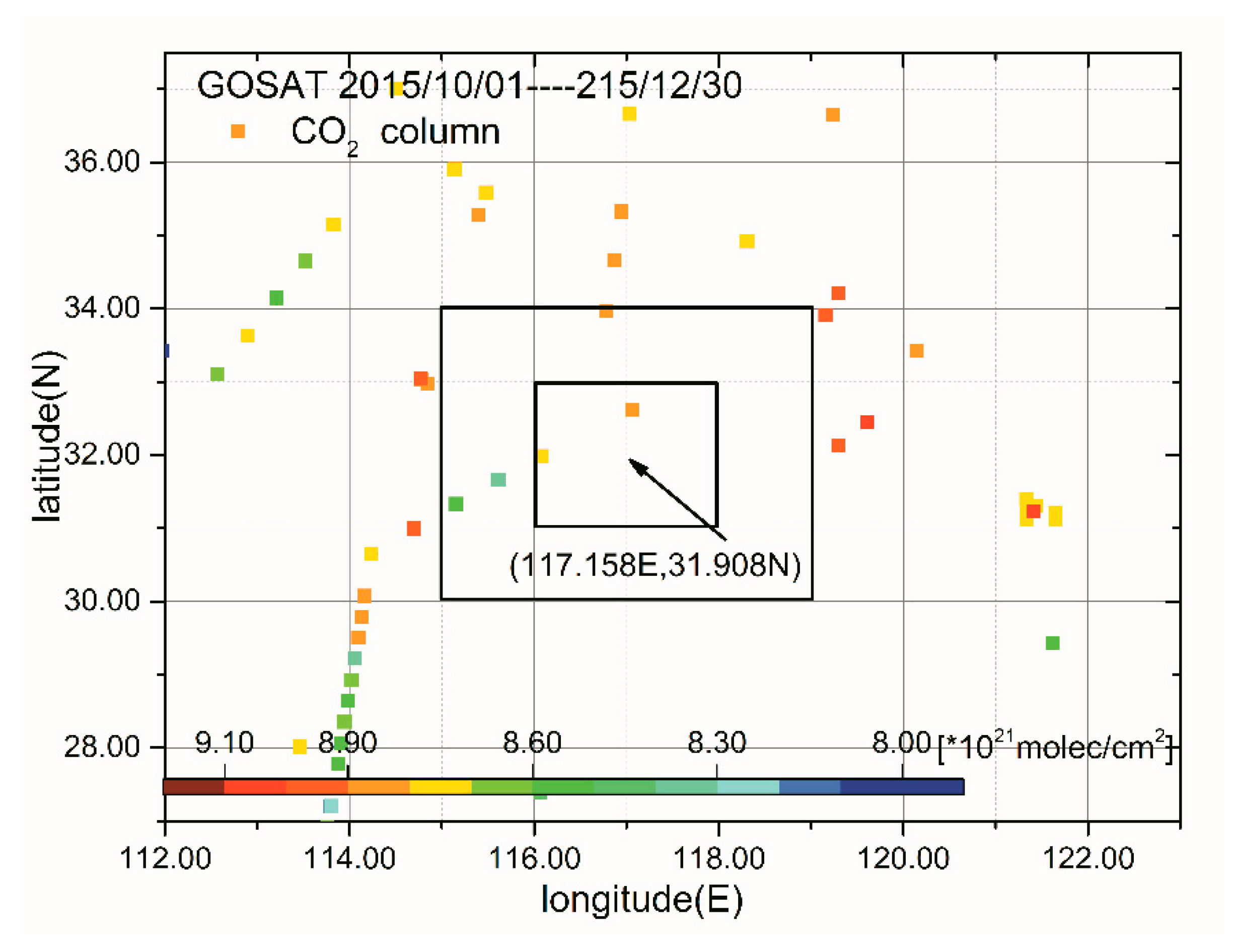
GOSAT CO2 total column from October to December, 2016, for a specific ground pixel ((117.158 ± 5) °E, (31.908 ± 5) °N).
Figure 11.
GOSAT CO2 total column from October to December, 2016, for a specific ground pixel ((117.158 ± 5) °E, (31.908 ± 5) °N).

Figure 12.
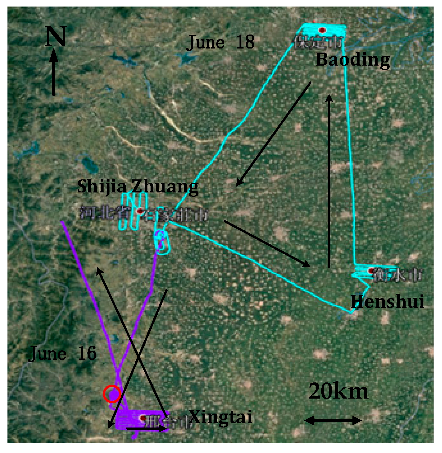
Flight trajectories of the airborne campaign: the line in purple represents the flight path on June 16, and the red circle indicates that the aircraft in the area is spiraling up and down; the line in blue represents the flight path on June 18, and the arrows represent the flight directions.
Figure 12.
Flight trajectories of the airborne campaign: the line in purple represents the flight path on June 16, and the red circle indicates that the aircraft in the area is spiraling up and down; the line in blue represents the flight path on June 18, and the arrows represent the flight directions.

Figure 13.
Time series of CO2 column, height, and retrieval errors during flight.

Figure 14.
Linear relationship between CO2 column and altitudes during spiraling up and plummeting down stages.
Figure 14.
Linear relationship between CO2 column and altitudes during spiraling up and plummeting down stages.

Figure 15.
Regional CO2 distribution of the four cities (Xing-tai, Baoding, Henshui, and Shijiazhuang) observed at 3 km by Air-IRSS.
Figure 15.
Regional CO2 distribution of the four cities (Xing-tai, Baoding, Henshui, and Shijiazhuang) observed at 3 km by Air-IRSS.

Figure 16.
(a) Functional zoning of Baoding; (b) wind speed and wind direction of Baoding during the flight experiment.
Figure 16.
(a) Functional zoning of Baoding; (b) wind speed and wind direction of Baoding during the flight experiment.


Table 1.
The input parameters for SCIATRAN.
| Lower and Upper Boundary for CWF Calculation | 120 km | Pressure and Temperature Profiles | Scaled US Standard |
|---|---|---|---|
| Number of altitude layers | 53 | Atmospheric profile | Scaled US standard |
| Time | 2016/6/18 | Trace gases | CO2, H2O, CH4 |
| Wavelength band | 1590.0~1620.0 nm | CWF integration mode | numeric |
| Internal wavelength step | 0.1 nm | Slit function FWHM | 0.45 nm |
| Scattering | Multiple | Slit function type | Gaussian |
| Latitude & longitude | 38.67°N, 115.45°E | Line absorber treatment | Line-by-line |
| Aerosol parameterization | LOWTRAN | Radiative transfer model | Pseudo-spherical |
| cloud | NO | Surface type | loam soil |
| SZA | 38° | Thermal emission | NO |
| Height above sea level | 3 km | Radiance | Relative |
Table 2.
Parameters for calculating sensitivity.
| Parameters | Variables |
|---|---|
| Aerosol | City (sunny), City (sunny after rain), Rural (sunny), Rural (sunny after rain) |
| Surface albedo | 0.2, 0.3, 0.4, 0.5, 0.6, 0.7 |
| Resolution (nm) | 0.4, 0.43, 0.45, 0.47, 0.5 |
| Zenith (°) | 10, 15, 20, 25, 30, 35, 40, 45 |
| Output height (km) | 2.5, 2.7, 2.9, 3.0, 3.1, 3.2 |
| Azimuth (°) | 90, 120, 150, 160, 180, 210, 240, 270 |
The bold variables are the actual parameters of the selected spectrum and are taken as the reference in the sensitivity calculations.
Table 3.
Parameter settings of two different vertical grid modes.
| Grid Mode | Aerosol | Surface Albedo | Resolution (nm) | Zenith (°) | Output Height (km) | Azimuth (°) |
|---|---|---|---|---|---|---|
| 50 layers | City (sunny) | 0.5 | 0.45 | 30 | 1,2,3,4,5,10,20 | 160 |
| 53 layers | City (sunny) | 0.5 | 0.45 | 30 | 1,2,3,4,5,10,20 | 160 |
Table 4.
Sensitivity to different types of aerosols.
| Aerosol Types | Sensitivity/CO2 [%] |
|---|---|
| Rural sunny after rain | 0.096 |
| Rural sunny | 0.044 |
| Urban sunny | 0.000 |
| Urban sunny after rain | 0.036 |
Table 5.
Sensitivity of CO2 column under the aircraft.
| Parameters | Sensitivity/% [CO2] | Parameters | Sensitivity/% [CO2] | ||
|---|---|---|---|---|---|
| SZA (°) | 10 | −4.520 | Albedo | 0.5 | 0.000 |
| 15 | −3.240 | 0.6 | +0.200 | ||
| 20 | −2.501 | 0.7 | +0.401 | ||
| 25 | −1.130 | Resolution (nm) | 0.4 | −0.080 | |
| 30 | 0.000 | 0.43 | −0.030 | ||
| 35 | 1.150 | 0.45 | 0.000 | ||
| 40 | 2.991 | 0.47 | +0.020 | ||
| 45 | 3.200 | 0.5 | +0.051 | ||
| Azimuth (º) | 160 | 0.000 | Altitude (km) | 2.5 | −1.420 |
| 90, 120, 150, 180, 210, 240, 270 | 0.000 | 2.7 | −1.190 | ||
| 2.9 | −0.480 | ||||
| Albedo | 0.2 | −0.600 | 3.0 | 0.000 | |
| 0.3 | −0.410 | 3.1 | +0.430 | ||
| 0.4 | −0.201 | 3.2 | +0.650 | ||
The bold variables are the actual parameters of the selected spectrum and are taken as the reference in the sensitivity calculations.
Table 6.
Total uncertainties to be estimated in a WFM-DOAS retrieval of CO2 total column.
| Parameter | Expected Variation (Airborne/Fixed) | Uncertainty CO2 [%] (Airborne/Fixed) |
|---|---|---|
| Aerosol | urban → rural/urban | 0.044/0 |
| SZA | ±5º/±3º | 1.150/0.600 |
| Albedo | 0.500 ± 0.100 | 0.200 |
| Resolution | 0.450 ± 0.010 | 0.010 |
| Aircraft altitude | ±100 m/±50 m | 0.480/0.220 |
| Total uncertainty estimate: | 1.26/0.30 | |
© 2019 by the authors. Licensee MDPI, Basel, Switzerland. This article is an open access article distributed under the terms and conditions of the Creative Commons Attribution (CC BY) license (http://creativecommons.org/licenses/by/4.0/).
Share and Cite
MDPI and ACS Style
Wang, R.; Xie, P.; Xu, J.; Li, A.; Sun, Y. Observation of CO2 Regional Distribution Using an Airborne Infrared Remote Sensing Spectrometer (Air-IRSS) in the North China Plain. Remote Sens. 2019, 11, 123. https://doi.org/10.3390/rs11020123
AMA Style
Wang R, Xie P, Xu J, Li A, Sun Y. Observation of CO2 Regional Distribution Using an Airborne Infrared Remote Sensing Spectrometer (Air-IRSS) in the North China Plain. Remote Sensing. 2019; 11(2):123. https://doi.org/10.3390/rs11020123
Chicago/Turabian StyleWang, Ruwen, Pinhua Xie, Jin Xu, Ang Li, and Youwen Sun. 2019. "Observation of CO2 Regional Distribution Using an Airborne Infrared Remote Sensing Spectrometer (Air-IRSS) in the North China Plain" Remote Sensing 11, no. 2: 123. https://doi.org/10.3390/rs11020123
Note that from the first issue of 2016, this journal uses article numbers instead of page numbers. See further details here.