Article

Using High-Spatiotemporal Thermal Satellite ET Retrievals for Operational Water Use and Stress Monitoring in a California Vineyard

1
USDA-ARS, Hydrology and Remote Sensing Lab, Beltsville, MD 20705-2350, USA
2
E & J Gallo Winery, Viticulture, Chemistry and Enology, Modesto, CA 95354, USA
3
NASA Marshall Space Flight Center, Huntsville, AL 35811, USA
4
USDA-ARS, National Laboratory for Agriculture and the Environment, Ames, IA 50011, USA
*
Author to whom correspondence should be addressed.
Remote Sens. 2019, 11(18), 2124; https://doi.org/10.3390/rs11182124
Submission received: 7 August 2019 / Revised: 6 September 2019 / Accepted: 9 September 2019 / Published: 12 September 2019
(This article belongs to the Special Issue Remote Sensing: 10th Anniversary)

Abstract

:
In viticulture, deficit irrigation strategies are often implemented to control vine canopy growth and to impose stress at critical stages of vine growth to improve wine grape quality. To support deficit irrigation scheduling, remote sensing technologies can be employed in the mapping of evapotranspiration (ET) at the field to sub-field scales, quantifying time-varying vineyard water requirements and actual water use. In the current study, we investigate the utility of ET maps derived from thermal infrared satellite imagery over a vineyard in the Central Valley of California equipped with a variable rate drip irrigation (VRDI) system which enables differential water applications at the 30 × 30 m scale. To support irrigation management at that scale, we utilized a thermal-based multi-sensor data fusion approach to generate weekly total actual ET (ETa) estimates at 30 m spatial resolution, coinciding with the resolution of the Landsat reflectance bands. Crop water requirements (ETc) were defined with a vegetative index (VI)-based approach. To test capacity to capture stress signals, the vineyard was sub-divided into four blocks with different irrigation management strategies and goals, inducing varying degrees of stress during the growing season. Results indicate derived weekly total ET from the thermal-based data fusion approach match well with observations. The thermal-based method was also able to capture the spatial heterogeneity in ET over the vineyard due to a water stress event imposed on two of the four vineyard blocks. This transient stress event was not reflected in the VI-based ETc estimate, highlighting the value of thermal band imaging. While the data fusion system provided valuable information, latency in current satellite data availability, particularly from Landsat, impacts operational applications over the course of a growing season.

1. Introduction

Efficient use of agricultural water resources through irrigation scheduling is predicated on the accurate prediction and constant monitoring of evapotranspiration (ET) at the field or sub-field scale. This is especially true in viticulture, where both the amount and timing of irrigation applications are specifically used to control vine growth and manage grape yield and quality [1,2,3,4,5,6,7]. Consequently, growers closely monitor vineyard water status relative to a phenologically varying target water status goal, modifying irrigation amounts accordingly. Numerous methods exist to determine vineyard ET and to infer water status/use, including both ground- and satellite-based remote sensing solutions. Ground-based solutions can offer reliable, localized ET estimates; however, their utility is limited by high maintenance cost and challenges in upscaling to the vineyard or multi-vineyard scale. Satellite-based remote sensing methods, on the other hand, routinely provide spatial information useful for determining regional to field scale heterogeneity in vine conditions and water status, making them more suitable for large-area management. Given the free and open data access policies applicable to many earth-observing satellites, growers understand the potential of satellite-based remote sensing for effective assessment of water status at serviceable spatial and temporal scales and are beginning to apply these technologies operationally.
In addition to actual water consumed, irrigation scheduling also requires an estimate of the water required to maintain optimal crop health. One common and practical approach for the estimation of crop water requirements is the application of the Food and Agriculture Organization’s (FAO) Irrigation and Drainage Paper No. 56 [8] method. This method has been widely used to estimate water use and schedule irrigation [8,9] and is often preferred due to its simplicity and ability to be applied operationally. The FAO-56 method derives an estimate of crop evapotranspiration (ETc) under standard conditions (i.e., well-watered, well-fertilized and disease-free) from the product of the reference ET (ETo) and a crop coefficient (Kc). Kc represents characteristics that distinguish the crop from grass reference, including crop height, albedo, canopy resistance and evaporation from the soil. Depending on the accuracy required and/or data availability, the crop coefficient can represent the time averaged combined effects of crop transpiration and soil evaporation (Kc), or separated into two coefficients, the basal crop coefficient (Kcb; describing plant transpiration) and soil evaporation coefficient (Ke; describing soil evaporation) [8]. ETo is often calculated using the FAO-Penman Monteith equation, which is recommended by the FAO as the standard method [8], and represents the effects of weather conditions on the evapotranspiration process.
Standard values and temporal evolution of Kc values have been investigated for different crops and under different climate conditions [8,10]. However, because of dependencies on local climate and crop conditions, the implementation of generalized Kc values recommended by FAO-56 can lead to errors in estimated ET. In response, satellite-based remote sensing in the visible and near-infrared ranges have been shown to provide an indirect estimate of Kc over many surfaces [3,4,11,12,13,14,15,16,17,18,19,20]. Specifically, Reference [3] applied vegetation indices (VI)-based Kc values to determine actual ET (ETa) based on the FAO-56 approach within a vineyard located in southeastern Spain. However, the determination of ETa (and not ETc) through the FAO-56 approach requires an additional adjustment to Kc to account for water stress in the root zone. This adjustment is dependent on irrigation and precipitation information, as well as soil physical water retention properties. Calculating such an adjustment and scaling it to multiple vineyards from an operational standpoint is challenging as detailed soil and rooting depth information is not reliably available over the landscape. Moreover, prior irrigation information is very difficult to obtain, particularly over multiple vineyards and in near real time for making operational decisions. In addition, satellite-derived VIs are slow to respond to plant stress, making them less useful for monitoring rapid changes in crop water use [21,22]. This is especially pertinent in a vineyard setting, where vines are purposely being grown in a semi-stressed state during certain phenological stages.
In contrast, thermal infrared (TIR) imagery and derived land-surface temperature (LST) conveys spatially explicit signals of actual water use and stress without the need for a priori information on soil water retention properties, rooting depth, precipitation or irrigation [23,24]. LST also provides a faster response signal of incipient stress than VI methods, allowing for timely mapping of transient stress signals [25]. The TIR-based Atmosphere-Land Exchange Inverse (ALEXI) [26,27,28] surface energy balance model and associated flux disaggregation technique (DisALEXI) [29,30] uses LST derived from TIR imagery to map ETa. The regional ALEXI model is run operationally over CONUS at 4-km resolution, exploiting the sub-hourly TIR imagery collected by the Geostationary Operational Environmental Satellites (GOES). DisALEXI can be used to downscale the ALEXI fluxes over target areas of interest at high-spatial/low-temporal (e.g., using Landsat) and at moderate-spatial/high-temporal (e.g., using the Moderate Resolution Imaging Spectroradiometer; MODIS) resolution. Landsat and MODIS ETa retrievals are then merged using a data fusion methodology (Spatial and Temporal Adaptive Reflectance Fusion Model; STARFM) [31] to create ET datacubes with both high spatial (30 m) and temporal (daily) resolutions [32]. In this approach, the MODIS ET retrievals are effectively used to inform interpolation between Landsat overpasses and, in operational mode, extrapolation beyond the last available overpass.
This thermal-based approach has been successfully applied over multiple landcover types [23,32,33,34,35,36,37,38], including vineyards [39,40]. The vineyard-specific applications of the ALEXI/DisALEXI modeling scheme demonstrated utility in monitoring vine water use and stress, capturing within-vineyard spatial heterogeneity of ETa and matching tower observations. An additional benefit of the ALEXI/DisALEXI approach for irrigation operational management is that it does not require ground-based or site-specific data, making it scalable to surrounding vineyards. However, applications of ALEXI/DisALEXI to date have been conducted in a retrospective manner, meaning all required satellite-remote sensing data were available up to and beyond the final modeling date. This allows the use of reprocessed and evaluated satellite imagery that meets defined quality standards. For operational applications, the lag time in satellite-remote sensing data availability (latency) needs to be addressed.
Satellite-based remote sensing of ETa at 30-m resolution can facilitate precision irrigation management. Typically, a vineyard block is irrigated to the demands of a desirable part of the block, meaning the remaining vines may be over- or under-irrigated. New irrigation technology, such as variable rate drip irrigation (VRDI) systems, provide differential water delivery to sub-blocks within the field, allowing the tailoring of irrigation amounts to the specific water demands of each sub-block. Remote sensing enables mapping of the spatial variability in water demand, allowing better regulation of vine growth via irrigation over smaller areas. The goals of VRDI are to produce more homogeneous yields over a vineyard, to improve grape quality by reducing over/under irrigation, and to reduce overall water use.
In the current study, we investigate the capabilities of currently operational VI-based ETc (FAO-56 method) and the thermal-based ETa (ALEXI/DisALEXI + STARFM method) for operational irrigation decision support at sub-field scales. The thermal-based ETa approach is run for the first time in an operational setting permitting an evaluation of its capability to detect stress, the timeliness of the ETa product, and what the current limitations that need to be addressed are for future operational water use monitoring applications using satellite data. This study was conducted over a VRDI-equipped vineyard divided into four sections, each receiving different levels of deficit irrigation to induce varying levels of stress. During the 2018 growing season, both ETa and ETc were computed at weekly time steps every week over the vineyard and compared with flux observations collected at flux tower sites installed within each section. In addition, the spatiotemporal responsiveness of ETa and ETc to imposed stress patterns was evaluated considering known satellite data latencies.

2. Materials and Methods

2.1. Study Domain

The study was conducted between the months of May and October of 2018 over a vineyard located 25 km west of Fresno, California, using data collected as part of the USDA-ARS grape remote sensing atmospheric profile and evapotranspiration experiment (GRAPEX) [41]. The vineyard was planted in 2010 with Merlot (Vitis vinifera L.) vines trained to quadrilateral cordons on a horizontally split trellis. Vines were spaced 1.5 m apart with 3.35 m row spacing and east-west row orientation. The vineyard has an area of 16 ha and experiences a warm Mediterranean climate characterized by abundant sunshine and large day-to-night temperature differences. Degree day (DD) accumulations for the growing season are typically 4200 DD. Total precipitation and average air temperature measured between May and October of 2018 were 12 mm and 22 °C, respectively. The entire vineyard is characterized by sandy loam and a 0–1 percent slope. The vineyard is equipped with a variable rate drip irrigation (VRDI) system (black grid; Figure 1) capable of applying specific amounts of irrigation on a 30 × 30 m gridded basis [42]. This grid was designed to have a symmetrical arrangement from the middle North-South line of the field so that each multi-tube drip irrigation bundle would span six pixels either from the west or from the east edges, where the valve boxes were located. We further divided the vineyard into four separate sections (blue grid; Figure 1), each equipped with a dedicated easy covariance flux tower (red dots), to test model response to varying stress levels within the vineyard. Flux tower placement was determined through footprint analysis, outlined in Reference [43], using data from a nearby vineyard also part of the GRAPEX project [41]. Specifically, daytime data collected during the growing season indicated wind from the northwest quadrant nearly 95% of the time with a median wind direction of 317°. The median upwind extent of the footprint was 48 m, while the maximum upwind extent was 78 m. Therefore, flux towers were placed in the southeast corner of each block to maximize fetch within the block. More details pertaining to treatment selection are presented in the following section.

2.2. Field Measurements

Micrometeorological and biophysical field measurements collected during GRAPEX were designed to serve as validation for modeled ETa estimates, detect vine stress, and monitor biomass development and root zone soil water availability. Each of the four vineyard sections was equipped with identical micrometeorological instrumentation and started recording in early May of 2018. The towers were located in the SE corner of each block to maximize fetch within the block, with winds predominantly from the northwest. Data collected include high frequency (20 Hz) and mean (half-hourly) measurements of three-dimensional wind, temperature water vapor and CO2. Net radiation and soil heat flux measurements, together with sensible and latent heat (turbulent) fluxes derived from the 20 Hz data, provided surface energy balance observations. Volumetric water content was also measured at three depths (30 cm, 60 cm and 90 cm) along two transects perpendicular to vine row. One transect was located 25 cm east of the irrigation line emitter, and the other was 25 cm west. Reported soil moisture estimates are the average of the two transects.
Eddy covariance (EC) measurements of the turbulent fluxes were made by a Campbell Scientific, Inc. (Logan, USA) IRGASON water vapor/carbon dioxide sensor, which fully integrates the open-path analyzer and sonic anemometer. EC systems were mounted 4 m above local ground level (a.g.l.) facing due west and collect data at 20 Hz producing 30 min averages. The EC data were processed using the CSI EasyFlux software producing 30 min fully processed turbulent fluxes of sensible and latent heat. Additional instrumentation included: An NR01 net radiometer (Campbell Scientific, Inc.) mounted 4.35 m a.g.l.; an EE08 temperature and relative humidity sensor in aspirated shield (Apogee) mounted 4 m a.g.l.; and five HFT3.1 soil heat flux plates (Radiation and Energy Balance Systems) at −8 cm depth, with soil thermocouples at 2 and 6 cm depth and volumetric water content using Stevens Hydra-probe (see Reference [41] for details of the eddy flux system design). The soil profile measurements were made using water content reflectometers (Campbell Scientific model CS655) and sampled every 15 min. Comparisons of water content derived from gravimetric samples indicated that the CS655 measurements were reliable for the soils that existed in the VRDI vineyard. In 2018, soil moisture profiles measurements were made in blocks 1, 2 and 4, but not in block 3. The use of trade, firm, or corporation names in this article is for the information and convenience of the reader. Such use does not constitute official endorsement or approval by the US Department of Agriculture or the Agricultural Research Service.
During the period of study, average energy balance closure ratios (H + LE)/(Rn-G) were on the order of 0.91. Despite low closure errors, crop water use in irrigated areas in semi-arid regions can be influenced by advective conditions. Horizontal advection of hot/dry air can increase the evaporative demand over an irrigated vineyard, causing latent heat flux values to exceed the available energy (Rn-G). Consequently, the additional energy required to meet atmospheric demand is extracted from the air above the canopy, resulting in negative sensible heat. Additionally, horizontal advection complicates the eddy covariance measurements by providing a horizontal contribution to the flux measurements [44]. Therefore, daily latent heat estimates with closure errors on the order of 20% or more are omitted from the analysis. Observed latent heat fluxes were corrected for closure errors using the residual (RE) method described in Reference [45].

2.3. ET Remote Sensing Framework and Irrigation Strategy

2.3.1. Vineyard Irrigation Strategy

To test the sensitivity of the satellite ET retrievals to differences in canopy stress, the northern blocks (blocks 1 and 2) in the experimental vineyard were subjected to a controlled stress event. This was accomplished by withholding irrigation during a portion of the early growing season until the soil water in the root zone was depleted, and there were visible and measurable signs of stress observed on the ground, such as repressed shot tip growth, leaf water potentials below −1.5 MPa, and leaf senescence. Shortly after this stress was accomplished, irrigation recommenced at a rate roughly equal to a grass reference ET to avoid major negative impacts on vine and berry health. The southern blocks (blocks 3 and 4) were chosen to receive normal deficit irrigation amounts and to experience typical target stress conditions as supported by leaf water potential measurements. Irrigation amounts within these blocks were determined through a combination of visual and locally-sourced data techniques by resident vineyard managers. This experimental setup allows comparison between stressed vines and irrigated vines following common practices, i.e., a business-as-usual approach.

2.3.2. Thermal-Based ETa Estimation

Throughout the growing season, weekly ETa estimates were delivered to the VRDI irrigation manager each Friday morning (product delivery date), representing the summation of daily ETa from the prior Friday to Thursday. The Thursday end of the weekly compositing interval is hereafter referred to as the effective weekly product date.
Routine spatial information from satellite remote sensing techniques was used to generate daily 30 m ET estimates over the study domain. Modeled ET estimates were updated each Friday during the growing season using the latest available satellite imagery and techniques to project forward to the effective product date. Weekly sums of ET were then computed and sent to vineyard managers for assessment. While the projection technique used to project forward ET data where satellite data were absent is standard, quality and responsiveness are strongly dependent on the latency of the last available satellite image used.
The current study utilized the Atmosphere-Land Exchange Inverse (ALEXI) surface energy balance model [26] and the associated disaggregation algorithm (DisALEXI) [29,30] in combination with the Spatial and Temporal Adaptive Reflectance Fusion Model (STARFM) [31] to generate high spatiotemporal resolution ET time series maps. ALEXI is driven by time-differential land surface temperature (LST) observations acquired from geostationary satellites (GOES-East and GOES-West Imager instruments). Daily coarse-scale (4 km) ET fluxes from ALEXI are spatially downscaled (DisALEXI) to finer scales using higher resolution LST information from polar-orbiting systems MODIS (1 km) and Landsat (30 m). STARFM then combines the spatial resolution of Landsat with the temporal frequency of MODIS to produce the high spatiotemporal (30 m, daily) resolution ET time series. The reader is referred to References [23,31,32,33,35,40] for detailed descriptions of the components of this system. Previous applications of the DisALEXI and STARFM modeling framework have been completed in a retrospective manner; meaning all required datasets are available up to and beyond the final modeling date. In the current study, the DisALEXI and STARFM models were completed once a week, every week, during the growing season, requiring address of issues related to latency in satellite retrieved datasets.
At present, the ALEXI model is run operationally over the continental United States (CONUS) at 4 km resolution using LST retrieved using 11 µm brightness temperature observations from the GOES satellites. Raw brightness temperature observations are atmospherically corrected using atmospheric profiles of temperature, as outlined in Reference [46]. ALEXI also uses daily 4 km leaf area index (LAI) estimates interpolated and aggregated from the 500 m MODIS MCD15A3H 4-day product, governing partitioning of LST between soil and canopy temperature components. These 4-km daily ALEXI products are generated with a latency of two days.
In this study, the 4 km ALEXI products were spatially disaggregated with the DisALEXI algorithm to generate moderate (500 m) and high (30 m) resolution maps of ET using TIR imagery from MODIS (Terra satellite) and Landsat, respectively. Specifically, moderate resolution maps are generated by combining multiple standard MODIS products, including instantaneous swath products MOD11_L2 (LST) and MOD03 (geolocation). Bowtie effects due to off-nadir pixel smearing were reduced by applying the DMS procedure [47] using the MODIS 500 m composite MOD13A1 NDVI product [32,39]. In addition, DisALEXI-MODIS used daily LAI maps created using MODIS 4-day composite (MCD15A3H, Collection 6) products and a procedure outlined in Reference [48]. Composite images are smoothed and gapfilled to daily timesteps using the TIMESAT algorithm [49]. Input MODIS albedo maps were generated from the MODIS daily composite Bidirectional Reflectance Distribution Function (BRDF) 500-m spatial resolution (MCD43A3, Collection 6) product. MODIS LAI and albedo products have a typical latency of 2–6 or 9–10 days, respectively. These inputs were held constant at values derived from last available images to the date of the most recent thermal product (MOD11_L2), which has a current latency of fewer than two days, aligning with latency on the ALEXI ET dataset. Therefore, DisALEXI-generated moderate resolution maps of ET also have an effective two-day latency.
DisALEXI was also used to create high spatial resolution (30 m) maps of ET on Landsat 8 overpass dates. Landsat thermal band data at a native resolution of 100 m were atmospherically corrected using MODTRAN [50] then sharpened to 30 m resolution to match Landsat optical bands using the data mining sharpener (DMS) approach [47]. In the current study, we used Landsat 8 (L8) tier 1 (T1) data within one scene (path 43, row 34). Landsat 7 data were not used in this study due to image gaps caused by the scan-line corrector failure that occurred in 2013, which cross directly through the vineyard under study. L8 has a 16-day revisit cycle. Landsat T1 data product availability date was inconsistent, with a 21.6-day latency period, on average, during the 2018 growing season (Figure 2). Latency is measured as the number of days between the ET product delivery date (Friday of each week) and the last available L8 image (Figure 2; gray bars).
Landsat-based maps of ET were fused with the daily MODIS ET maps using STARFM, creating daily 30 m resolution maps of ET with a two-day latency (determined by the MODIS ET time series). The final two days of the weekly composite (Wednesday and Thursday) were computed by preserving the ratio between modeled ET on the last available day and locally sourced reference ET. This ratio map was then multiplied by the locally sourced reference ET value measured over the final two days. Grass reference ET (ETo) values were obtained from the local Fresno State CIMIS station (see further information in Section 3.3). All ET maps during that week were then summed to create a total weekly estimate of actual ET (ETa). This process, and subsequent product, is henceforth referred to as ETa-OP (operational) in the manuscript.
A fundamental advantage of the data fusion approach is the ability to reconstruct changes in surface conditions occurring at the 500-m scale between Landsat overpass dates. This is crucial given the semi-stressed state wine grapes are grown under, making them vulnerable to the rapid onset of stress. Moreover, ETa-OP is diagnosed from the LST signal, allowing for a better understanding of plant available water at sub-field resolution when compared to visible, near-infrared or passive microwave signals. It is also important to note that the ETa-OP approach estimates actual ET, which, in the absence of rainfall, irrigation and prior depletion of soil moisture reserves from observations, can be used as a proxy for applied irrigation. This can act as an important check on the amount of water being applied to the vineyards when irrigation data are not available.
In addition to this operational implementation, the DisALEXI + STARFM ET fusion modeling scheme was executed in a retrospective manner (henceforth referred to as ETa-retro) to serve as a baseline comparison for ETa-OP. Previous studies have shown the ET fusion model is capable of reasonably reproducing tower observations and capturing spatial heterogeneity of vineyard ET when completed in a retrospective manner where all satellite-derived parameters are available, bracketing the study period on both ends [39,40]. Comparisons of ETa-OP and ETa-retro model results allows assessment of operational capabilities and associated errors due to data latency.

2.3.3. Vegetation Index-Based ETc Estimation

While ETa describes actual water used by the vineyard, the crop water requirement, ETc, represents the upper limit of water that would be used by the crop under standard conditions, i.e., no water shortage, disease, or pressures related to weed, insect or salinity [8]. ETc estimates are actively being used in the viticulture community to determine irrigation amounts and monitor vineyard water requirements. In this study, ETc was computed for comparison with the actual water use, ETa-OP, computed once a week. The current study utilizes the modified Food and Agriculture Organization (FAO-56) [8] method based on satellite-derived vegetation indices to derived daily 30 m resolution maps of ETc.
ETc = Kc × ETo
In Equation (1), ETo is a grass reference ET obtained from a local CIMIS (California Irrigation Management Information System) weather station. Specifically, we use the Fresno State #80 station located near Fresno, CA (36.8208, −119.7423). CIMIS was developed by the California Department of Water Resources (DWR) and the University of California, Davis (UC Davis) to assist irrigators in managing their water resources more efficiently, with more than 140 automated weather stations located throughout California. CIMIS ETo is calculated using a modified Penman-Monteith equation [51] that assumes a well-watered grass surface. It also uses a wind function developed at UC Davis, and unique cloud factor values specific to each station.
Here we used a reflectance-based estimate of the crop coefficient, Kc, modulated by NDVI to capture seasonal variations in biomass and transpiration [52,53,54]
Kc = Ko × NDVI,
where Ko was determined empirically using flux observations collected within the VRDI vineyard and ETo obtained from the Fresno State CIMIS station. Tower flux observations in block 4 were used for this purpose as this block experienced the least amount of stress under the experimental design. Ko was computed using linear regression between Kc (the ratio of observed closure corrected ET, and CIMIS derived ETo; Equation (1)) and NDVI values averaged over a 3-by-3 pixel area (90 × 90 m) shifted northwest from the tower center to approximate the tower upwind fetch/footprint (see Figure 1) [12]. Analysis of linear regression forced through the origin reported a correlation coefficient of 0.59 and slope of 1.19 between NDVI and observed Kc values on Landsat overpass dates for block 4. Consequently, a Ko of 1.2 is used to calculate ETc via Equations (1) and (2). This value of Ko yields mid-season Kc values consistent with FAO-56 recommendations for wine grapes. Applying Equation (2) on Landsat overpass dates during the months of July and August resulted in Kc values between 0.78 and 0.82, while the FAO-56 mid-season Kc value (Kc-mid), adjusted for semi-arid conditions with an average wind speed of 3 m s−1, is 0.80. For more information into the determination of Kc, the reader is referred to References [3,17].
Equations (1) and (2) are becoming a common and convenient tool in viticulture to describe crop water requirements and to define an additional management factor required to reach a target stress level [3,55]. Its usage in the current study is to replicate standard practice through the utilization of NDVI from the most recent clear Landsat overpass combined with CIMIS ETo measurements. Although simple to implement and maintain, this standard practice can introduce errors by neglecting changes in canopy biomass that might occur between overpasses. These errors are likely to be exacerbated during the period of rapid vine growth that typically starts in early May and lasts through June. Furthermore, CIMIS ETo values are often from stations far removed from the vineyard site. Specifically, the Fresno State CIMIS station is located roughly 30 km from the vineyard. It is also important to note that CIMIS stations can and have gone offline mid-season, creating a void in ETo data, especially if the next closest CIMIS station to a vineyard of interest is much further away.

3. Results

3.1. Comparisons with Tower Observations

Weekly ET totals derived from the operational ET fusion model (ETa-OP) and the modified FAO-56 model (ETc) were given to irrigation managers during the growing season. ETa values were used to assess vine water use and stress and both ETa and ETc were used to assist in irrigation decision making, highlighting the importance of accuracy and timeliness in ET retrieval. Scatter plots of weekly total actual ET (ETa) from ETa-OP and ETa-retro in comparison with observations from towers (adjusted for closure, as described in Section 2.1) in all four blocks within the vineyard are shown in Figure 3. ETc from the modified FAO model is also compared, but typically falls above the one-to-one line as expected under conditions of stress. Statistical metrics of agreement between both operational and retrospective ETa retrievals and observations are provided in Table 1 and include both daily and weekly measurements in units of mm day-1. Metrics include mean observed and predicted values (Mean Obs and Mean Mod, respectively), coefficient of determination (R2), mean bias error (MBE), root mean square error (RMSE), mean average error (MAE) and percent error (% Error). The ETa-retro performance serves as a baseline (optimal data availability) for assessment of additional error introduced by data latency issues in real time. In all cases, modeled ET estimates (ETa-OP, ETc and ETa-retro) were averaged over a 3-by-3 pixel area (90 × 90 m) shifted northwest from tower center to approximate the typical tower upwind fetch/flux footprint.
ETa-OP and ETa-retro simulations show only a small difference in performance at the tower sites, with the retrospective simulation giving smaller errors in block 4, the operational simulation out-performing in blocks 1 and 2, and mixed performance in block 3. RMSE and MAE for both ETa-OP and ETa-retro improve when scaling from daily to weekly at each block due to time averaging of random errors. Daily MAE values range from 0.61 to 0.85 mm day−1 for ETa-retro and 0.71 to 0.82 mm day−1 for ETa-OP. These errors are on par with the target error of 0.80 mm day−1 suggested by Reference [56] for operational ET use. These errors also align with [39,40], where results from a baseline (retrospective) version of the ET fusion model were compared to flux tower estimates within a vineyard approximately 200 km north of the current study area. Similarities between ETa-OP and ETa-retro are encouraging, indicating the potential for operational applications of the ET fusion modeling system, an important step forward in delivering actionable water use/stress information to irrigation managers. However, temporal differences between operational and retrospective retrievals become more pronounced when the latency is increased between model completion date and satellite image acquisition (see Section 3.3).

3.2. Time Series Analysis

Time series of weekly total ETa-OP, ETa-retro, ETc and observed weekly total ET for the 2018 growing season at blocks 1, 2, 3 and 4 are shown in Figure 4 (bottom panels). Also included is the daily amount of applied irrigation within each block and daily measurements of soil moisture (volumetric water content, VWC; top panels) at 30 cm, 60 cm and 90 cm depth. Figure 4 highlights the general agreement between modeled weekly total ETa and observations and the decline of soil water availability during June and July. According to the experimental design, an additional stress was induced in the northern blocks (blocks 1 and 2) by withholding irrigation during an early portion of the growing season (14th June–23rd July) (Figure 4; top panels, yellow transparent rectangle). Blocks 3 and 4 received more uniform irrigation throughout the season, representing “business-as-usual” irrigation strategies. As previously mentioned, soil moisture sensors were not installed in block 3.
Observed and modeled weekly total ET estimates are lower at blocks 1 and 2 during the early portion of the growing season when compared to blocks 3 and 4, as expected. This difference is most pronounced during the months of June and July, as water availability decreased rapidly within the soil column due to the induced stressed. VWC progressively declined from June into July until all depths converged around 0.1 m3 m−3 at blocks 1, 2 and 4. Between weeks 19 July and 26 July, ETa-OP weekly total estimates decreased from 45 to 35 mm week−1 at blocks 1 and 2. ETa-retro weekly total estimates show a similar magnitude of decline, only two weeks prior. Conversely, ETc estimates remain relatively unchanged at 40 mm week−1 during the same period. The sharp decline in ETa-OP at the end of July aligns with observations of vine stress at the northern blocks by vineyard managers. However, the early detection in ETa-retro estimates agrees with the increased LST apparent in a Landsat scene on 12 July which was not available until the 27 July product delivery date in the operational runs. This may indicate a thermal stress signal occurring prior to the manifestation of visible effects. This is discussed in detail below. Following this stress event and the depletion of soil water availability, irrigation in blocks 1 and 2 was resumed (Figure 4, black bars) to improve vine conditions.
Restarting irrigation on 23 July had an immediate effect on VWC, with soil moisture doubling to 0.2 m3 m−3 and greater at the 30 cm depth. Although muted, VWC at 60 cm followed the general trend present at 30 cm depth. The lack of a significant response in VWC with irrigation at 90 cm suggests most of the water uptake took place at the upper soil layers, namely 60 cm and above. Despite withheld irrigation at blocks 1 and 2, the rapid and sustained increase in applied water during the remainder of the growing season yielded similar yearly total irrigation amounts at all blocks (block 1:326 mm, block 2:317 mm, block 3:322 mm, block 4:371 mm).

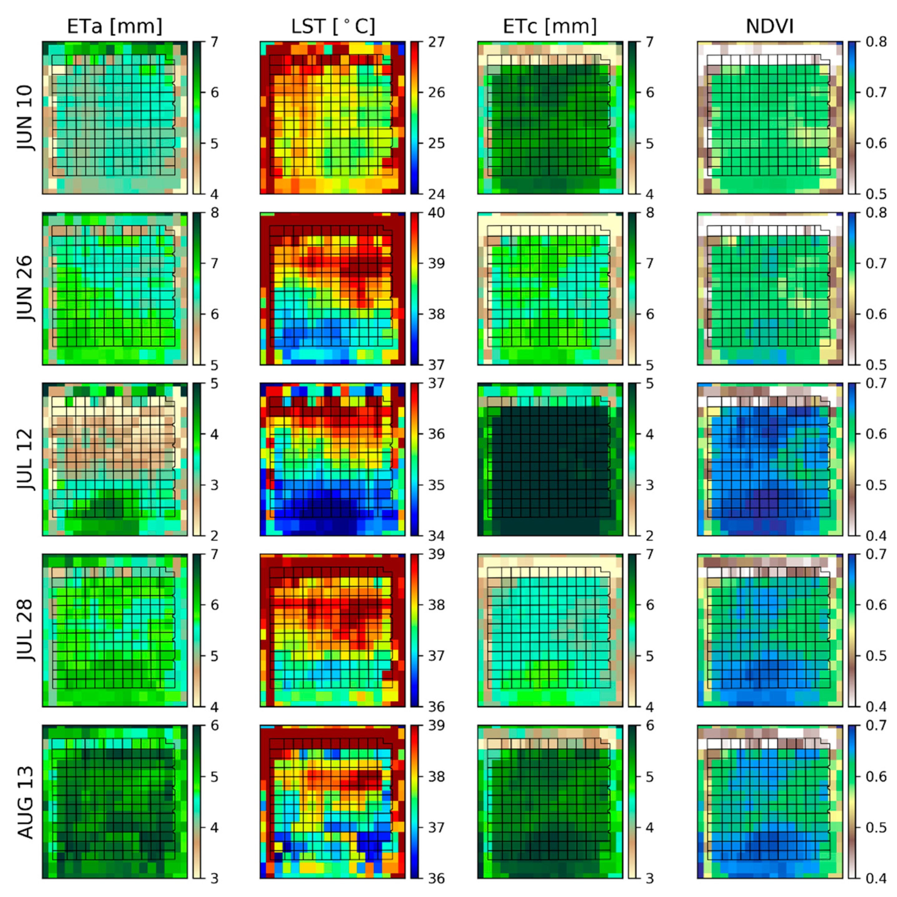
3.3. Spatial and Temporal Response to Irrigation and Stress

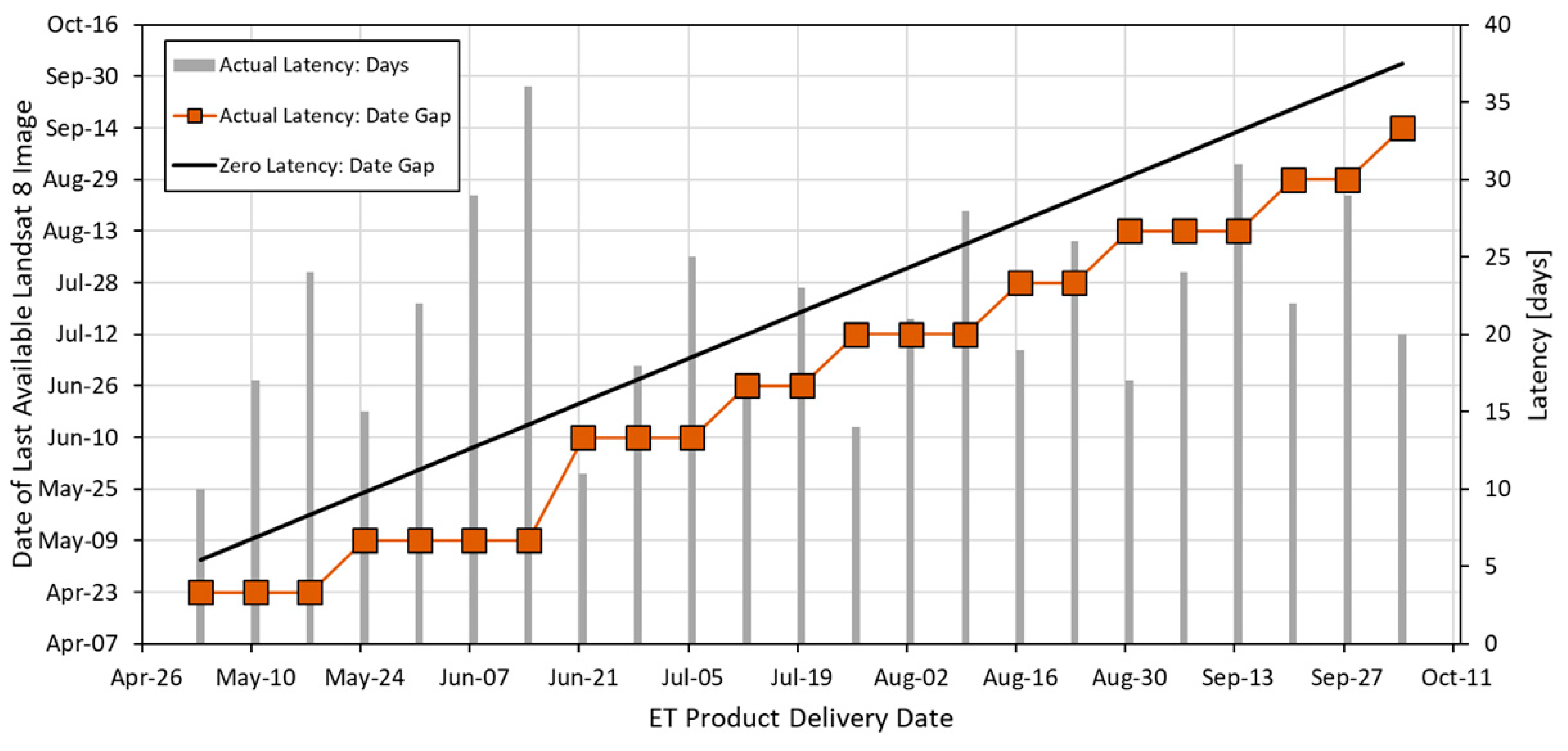
3.3.1. Landsat Overpass Dates

While Figure 4 demonstrates the response of both the physical system and the satellite ET retrievals to the induced stress at the tower locations, the response is even more apparent in viewing the vineyard spatially, particularly in the thermal remote sensing data. A sequence of maps of ETa-retro and ETc on Landsat 8 overpass dates during the stress and recovery period are shown in Figure 5, along with maps of LST and NDVI. Note that color scales in Figure 5 change between dates to highlight spatial heterogeneities; however, the magnitude of the color bar range is fixed. Maps of daily ETa-retro are spatially correlated to the LST imagery used as a key input variable in the DisALEXI modeling framework. Specifically, LST maps indicate elevated temperatures and lower ETa in the northern half of the vineyard beginning on 26 June, 12 days after irrigation suppression commenced in blocks 1 and 2. The distinct separation of LST and derived ETa was further enhanced in the next available Landsat image on 12 July, with an average ETa of 2.3 mm day−1 in the two northern blocks, and 3.2 mm day−1 in the south. As previously mentioned, stressed conditions over the northern half of the vineyard were first observed on the ground around 21 July, with irrigation restarted on 23 July to initiate recovery. The Landsat image time series suggests thermal signals of stress may have begun as early as 26 June and continued into the early portion of August, with peak stress occurring around 12 July.
In contrast to ETa and LST, the maps of ETc and NDVI (the only spatial input to ETc) do not indicate significant spatial discrepancies between the northern and southern portions of the vineyard for the Landsat overpass dates of 26 June or 12 July. The Landsat NDVI image on 28 July suggests a decrease in greenness over the northern vineyard blocks, leading to an 0.06 mm day-1 average difference in ETc on that date (Table 2). The observed flux differences between southern and northern tower sites were 1.29, 2.09 and 0.86 mm on 26 June, 12 July, and 28 July, respectively (Table 2). The spatial differences in ETa follow these observed trends, albeit smaller in magnitude, with differences increasing and peaking on 12 July. This spatial trend is missing in ETc (Table 2). The lack of spatial heterogeneity and delayed response to stress suggests that VNIR imagery and derived NDVI estimates may not suffice when monitoring stress in regions where rapid onset stress is commonplace.

3.3.2. Operational Application

Retrospective spatial analysis over Landsat overpass dates provides clear evidence that the ALEXI/DisALEXI modeling scheme, through the utilization of TIR imagery, is capable of detecting stress conditions at the field scale. Conversely, ETc estimates, derived using VNIR imagery, fail to capture the differences between the northern and southern blocks in the vineyard during the period of maximum stress. However, in operational applications, satellite data latency may obscure or delay detections of rapid stress onset.
Figure 6 depicts weekly total ET estimates derived from the ETa-OP, ETa-retro and ETc daily time series, along with the irrigation amounts applied with the VRDI system during each week. The date labels indicate the effective weekly product date (e.g., 14 June is the weekly total from 8 June to 14 June). Comparison between ETa-OP and ETa-retro provides evidence of issues related to latency in satellite data delivery. Most notably, indications of differential stress between north and south blocks of the vineyard are readily apparent on the 12 July weekly model run for ETa-retro, driven by the Landsat retrieval on that date (Figure 5). However, the same spatial differentiation between north and south portions of the vineyard is not realized in ETa-OP until the 26 July model run. This is because the 12 July Landsat 8 T1 image did not become available until 20 July—an 8-day lag between image acquisition and image download. This image was first incorporated in the July 26 weekly operational run. The net effect was an overall two-week latency in reported stress over the vineyard when compared to ETa-retro.
No considerable difference between northern and southern blocks is present in the weekly NDVI-driven ETc data during this period, although vineyard-wide average ETc slightly decreased for the 26 July model run when the 12 July Landsat NDVI image became available. The 16-day acquisition cycle of Landsat 8, combined with the 21.6-day latency in T1 product delivery (when measured from product delivery date), was not sufficient for timely capture of vegetation response to stress onset in this case.
Additional evidence for the need for timelier thermal image delivery is presented in Figure 7, showing the time variation in absolute error (orange triangles) between ETa-OP (average at all blocks) and observed weekly total ETa (average at all blocks) for each weekly model run. Transparent boxes indicate the dates when a new Landsat image became available in the operational model run. Model errors in ETa-OP generally increase between transparent boxes, as the last available Landsat image becomes more out of date. Updating the Landsat image (transparent boxes) typically leads to a notable decrease in error (blue boxes) for most model runs (Figure 7).

4. Discussion

4.1. Improvements in TIR Revisit and Data Latency

Although the thermal-based ETa-OP retrievals were successful in capturing spatial heterogeneity in ETa caused by local stress conditions, satellite revisits intervals and latency in data delivery remain an issue in an operational setting. Based on flux tower time series, Reference [57] suggest a return interval of five days or less is necessary to provide daily ET estimates with a relative error lower than 20% even if the retrievals are perfect. References [23,58] recommend a four-day or lower revisit cycle for improved temporal sampling to monitor ETa. Meeting these revisit targets will require integration of TIR data from multiple satellite platforms, and a reduction in data delivery latency must be realized.
Based on these results from 2018, modifications to the ETa data fusion processing stream in support of VRDI are being implemented in the 2019 growing season. Landsat 7 data are gapfilled and combined with Landsat 8 to reduce the potential interval for an update from 16 to 8 days. In addition, the real-time (RT) L8 thermal band products (typically available a few days after acquisition) have been downloaded and compared to the T1 products. The RT products are provisional, generated with estimated parameters for TIRS scene correction. While this will not always be so, the RT products compared well with the T1 products in these cases and could be used interchangeably without loss of fidelity.
Landsat 9, projected to launch no later than 2020, will follow the Landsat 7 orbit and will be capable of delivering corrected thermal products within a few days after acquisition [59]. NASA’s ECOsystem Spaceborne Thermal Radiometer Experiment on Space Station (ECOSTRESS) [60], deployed in July of 2018, collects multispectral thermal infrared data at 70 m resolution with an average revisit time of four days, providing a useful testbed for assessing the value of applying high spatiotemporal resolution TIR imaging. Future applications of the ETa-OP model will incorporate these new thermal image sources to improve operational capabilities and to create a more robust and reliable ETa toolkit for irrigation management and scheduling.

4.2. Value of Actual ET for Irrigation Management

Current viticultural irrigation practices are based on ETc and locally applied ‘management factors’ (Ko), which are specific to regions and varieties, and are used to control vegetative growth and apply some level of stress to meet fruit quality and yield targets. The ETa-OP model provides an improvement to this approach by measuring actual plant water use at sub-field resolutions. Quantifiable and direct water use estimates will offer a better way of determining available plant water and can act as an important check on applied irrigation. Also, ETa-OP will be used in conjunction with remotely-sensed reference ET to provide a spatially varying metric of vine stress. The ratio of ETa over reference ET will be used to account for changes in atmospheric demand, as well as to determine a level of vine water deficit and desired water stress levels. Because of its resolution, ETa data would be especially valuable in VRDI systems, where irrigation is applied differentially to each irrigation zone in order to decrease variability in vine vigor, fruit yield and quality.

5. Conclusions

Irrigation decision support driven by timely and accurate moderate resolution (30 m) satellite retrievals of actual ET have the potential for reducing water consumption in irrigated vineyards, while simultaneously improving yield and grape quality. This study explored the operational capabilities of a thermal-based (ETa-OP) ET data fusion model to reliably estimate ETa and determine associated water use and stress within a vineyard. Irrigation was withheld over the northern half of the vineyard to induce stress and to determine whether the ET models could detect this stress operationally. Each model was completed once a week, every week, during the growing season and validated against four flux tower stations installed within the vineyard.
Results of the study indicate the potential for operational applications of the DisALEXI + STARFM fusion model (ETa-OP). ETa-OP estimates had an average RMSE and MBE of 0.95 mm day−1 and −0.17 mm day−1, respectively, between blocks. Percent error values were less than 20% at all blocks, despite the greater than 4-day thermal image update cycle as recommended by Reference [23,58]. Daily MAE values were also on par with the target error of 0.80 mm day−1 suggested by Reference [56] for operational ET uses. Estimates of crop water requirements (ETc) developed from a modified NDVI-based FAO method were unable to capture the rapid decline in vineyard ETa over blocks 1 and 2 during the stress event that took place in late July. In contrast, ETa-OP could detect the rapid decline in vineyard ETa at both daily and weekly time steps; but the response was delayed, due to latencies in the availability of key Landsat 8 products.
Spatial analysis between ETa-OP and ETc showed similar results. The ETa-OP model could detect the spatial heterogeneity between north and south portions of the vineyard caused by delayed irrigation and induced stress. ETc estimates, predicated on NDVI imagery for spatial diversity, could not. This is likely due to reliance on satellite-derived vegetation indices which are slow to respond to indicators of stress and are only available on Landsat overpass dates. Landsat currently provides global coverage every 16 days, but depending on cloud coverage, can be much lower. This is insufficient to reliably derive ETa information for water resources management, especially for a vineyard, where vines are typically managed at a semi-stressed state during certain phenological stages via deficit irrigation, and irrigation amounts are specific to local water use conditions. Also, a delayed or absent response to stress indicates visible/near-infrared approaches may not suffice when monitoring water use in near-real-time, especially in areas where surface conditions can change quickly. Consequently, the use of thermal infrared systems becomes paramount in real-time applications of stress detection and irrigation scheduling. While ETa-OP produces valuable spatial information, latency in current satellite data availability, particularly Landsat, impact operational applications over the course of a growing season. Current spaceborne missions are addressing this issue, providing the foundation for operational thermal infrared capabilities that will support agricultural management services and provide data for operational management-appropriate ET estimates.

Author Contributions

Conceptualization: K.R.K., W.P.K., M.C.A., M.M.A., L.A.S.; Data curation: F.G., M.C.A., C.R.H., J.G.A., J.H.P., L.G.M.; Formal analysis: K.R.K., W.P.K., M.C.A., M.M.A.; Investigation: K.R.K., W.P.K., M.C.A.; Methodology: K.R.K., W.P.K., M.C.A.; Validation: K.R.K., M.C.A.; Visualization: K.R.K., M.C.A.; Writing—original draft: K.R.K., M.C.A., W.P.K.; Writing—review and editing: K.R.K., W.P.K., M.C.A., J.G.A., F.G., L.A.S.

Funding

This research was funded by NASA Applied Sciences – Water Resources Program, grant number NNH17AE39I.

Acknowledgments

Funding and logistical support for the GRAPEX project was provided by E. & J. Gallo Winery and from the NASA Applied Sciences-Water Resources Program (Grant No. NNH17AE39I). In addition, we thank the staff of Viticulture, Chemistry and Enology Division of E. & J. Gallo Winery for the collection and processing of field data and the cooperation of the vineyard management staff at the Ripperdan Ranch for coordinating field operations during this study. USDA is an equal opportunity provider and employer.

Conflicts of Interest

The authors declare no conflict of interest.

References

  1. Heilman, J.; McInnes, K.; Gesch, R.; Lascano, R.; Savage, M. Effects of trellising on the energy balance of a vineyard. Agric. For. Meteorol. 1996, 81, 79–93. [Google Scholar] [CrossRef]
  2. Yunusa, I.A.M.; Walker, R.R.; Loveys, B.R.; Blackmore, D.H. Determination of transpiration in irrigated grapevines: Comparison of the heat-pulse technique with gravimetric and micrometeorological methods. Irrig. Sci. 2000, 20, 1–8. [Google Scholar] [CrossRef]
  3. Campos, I.; Neale, C.M.; Calera, A.; Balbontín, C.; González-Piqueras, J. Assessing satellite-based basal crop coefficients for irrigated grapes (Vitis vinifera L.). Agric. Water Manag. 2010, 98, 45–54. [Google Scholar] [CrossRef]
  4. Galleguillos, M.; Jacob, F.; Prevolt, L.; Lagacherie, P.; Liang, S.L. Mapping evapotranspiration over a Mediterranean vineyard watershed. IEEE Geosci Remote Sens. Lett. 2011, 8, 168–172. [Google Scholar] [CrossRef]
  5. Intrigliolo, D.S.; Castel, J.R. Effects of irrigation on the performance of grapevine cv. Tempranillo in Requena, Spain. Am. J. Enol. Viticult. 2008, 59, 30–38. [Google Scholar]
  6. Shellie, K.C. Vine and berry response of merlot (Vitis vinifera L.) to differential water stress. Am. J. Enol. Viticult. 2006, 57, 514–518. [Google Scholar]
  7. Sivilotti, P.; Bonetto, C.; Paladin, M.; Peterlunger, E. Effect of soil moisture availability on Merlot: From leaf water potential to grape composition. Am. J. Enol. Viticult. 2005, 56, 9–18. [Google Scholar]
  8. Allen, R.G.; Pereira, L.S.; Raes, D.; Smith, M. Crop Evapotranspiration. In Guidelines for Computing Crop Water Requirements-FAO Irrigation and Drainage Paper 56; FAO: Rome, Italy, 1998. [Google Scholar]
  9. Pereira, L.S.; Allen, R.G.; Smith, M.; Raes, D. Crop evapotranspiration estimation with FAO56: Past and future. Agric. Water Manag. 2015, 147, 4–20. [Google Scholar] [CrossRef]
  10. Wright, J.L. New evapotranspiration crop coefficients. J. Irrig. Draingae Div. 1982, 108, 57–74. [Google Scholar]
  11. Jackson, R.D.; Idso, S.B.; Reginato, R.J.; Pinter, P.J. Remotely sensed crop temperatures and reflectances as inputs to irrigation scheduling. In Irrigation and Drainage: Today’s Challenges; ACSE: New York, NY, USA, 1980; pp. 390–397. [Google Scholar]
  12. Bausch, W.C.; Neale, C.M.U. Crop Coefficients Derived from Reflected Canopy Radiation: A Concept. Trans. ASAE 1987, 30, 703–709. [Google Scholar] [CrossRef]
  13. Choudhury, B.; Ahmed, N.; Idso, S.; Reginato, R.; Daughtry, C. Relations between evaporation coefficients and vegetation indices studied by model simulations. Remote Sens. Environ. 1994, 50, 1–17. [Google Scholar] [CrossRef]
  14. Hunsaker, D.J.; Pinter, P.J.; Barnes, E.M.; Kimball, B.A. Estimating cotton evapotranspiration crop coefficients with a multispectral vegetation index. Irrig. Sci. 2003, 22, 95–104. [Google Scholar] [CrossRef]
  15. Hunsaker, D.J.; Pinter, P.J.; Kimball, B.A. Wheat basal crop coefficients determined by normalized difference vegetation index. Irrig. Sci. 2005, 24, 1–14. [Google Scholar] [CrossRef]
  16. Duchemin, B.; Hadria, R.; Er-Raki, S.; Boulet, G.; Maisongrande, P.; Chehbouni, A.; Escadafal, R.; Ezzahar, J.; Hoedjes, J.; Kharrou, M.; et al. Monitoring wheat phenology and irrigation in Central Morocco: On the use of relationships between evapotranspiration, crops coefficients, leaf area index and remotely-sensed vegetation indices. Agric. Water Manag. 2006, 79, 1–27. [Google Scholar] [CrossRef]
  17. Er-Raki, S.; Chehbouni, A.; Guemouria, N.; Duchemin, B.; Ezzahar, J.; Hadria, R. Combining FAO-56 model and ground-based remote sensing to estimate water consumptions of wheat crops in a semi-arid region. Agric. Water Manag. 2007, 87, 41–54. [Google Scholar] [CrossRef] [Green Version]
  18. Er-Raki, S.; Chehbouni, A.; Boulet, G.; Williams, D.G. Using the dual approach for FAO-56 for partitioning ET into soil and plant components for olive orchards in a semi-arid region. Agric. Water. Manag. 2010, 97, 1769–1778. [Google Scholar] [CrossRef]
  19. Carrasco-Benavides, M.; Ortega-Farías, S.; Lagos, L.O.; Kleissl, J.; Morales, L.; Poblete-Echeverría, C.; Allen, R.G. Crop coefficients and actual evapotranspiration of a drip-irrigated Merlot vineyard using multispectral satellite images. Irrig. Sci. 2012, 30, 485–497. [Google Scholar] [CrossRef]
  20. Kamble, B.; Kilic, A.; Hubbard, K. Estimating Crop Coefficients Using Remote Sensing-Based Vegetation Index. Remote Sens. 2013, 5, 1588–1602. [Google Scholar] [CrossRef] [Green Version]
  21. Moran, M.S. Thermal Infrared Measurements as an Indicator of Plant Ecosystem Health. In Thermal remote sensing in land surface processes; Quattrochi, D.A., Luvall, J., Eds.; Taylor & Francis: Philadelphia, PA, USA, 2003; pp. 257–282. [Google Scholar]
  22. Glenn, E.P.; Huete, A.R.; Nagler, P.L.; Nelson, S.G. Relationship Between Remotely-sensed Vegetation Indices, Canopy Attributes and Plant Physiological Processes: What Vegetation Indices Can and Cannot Tell Us about the Landscape. Sensors 2008, 8, 2136–2160. [Google Scholar] [CrossRef]
  23. Anderson, M.C.; Allen, R.G.; Morse, A.; Kustas, W.P. Use of Landsat thermal imagery in monitoring evapotranspiration and managing water resources. Remote Sens. Environ. 2012, 122, 50–65. [Google Scholar] [CrossRef]
  24. Hain, C.R.; Crow, W.T.; Anderson, M.C.; Yilmaz, M.T. Diagnosing neglected moisture sources/sink processes with a thermal infrared-based Two-Source Energy Balance model. J. Hydrometeorol. 2015, 16, 1070–1086. [Google Scholar] [CrossRef]
  25. Otkin, J.A.; Anderson, M.C.; Hain, C.; Mladenova, I.E.; Basara, J.B.; Svoboda, M. Examining Rapid Onset Drought Development Using the Thermal Infrared–Based Evaporative Stress Index. J. Hydrometeorol. 2013, 14, 1057–1074. [Google Scholar] [CrossRef]
  26. Andserson, M.C.; Norman, J.M.; Diak, G.R.; Kustas, W.P.; Mecikalski, J.R. A two-source time integrated model for estimating surface fluxes using thermal infrared remote sensing. Remote Sens. Environ. 1997, 60, 195–216. [Google Scholar] [CrossRef]
  27. Anderson, M.C.; Norman, J.M.; Kustas, W.P.; Li, F.; Prueger, J.H.; Mecikalski, J.R. A climatological study of evapotranspiration and moisture stress across the continental United States: I. Model formulation. J. Geophys. Res. 2007, 112, D10117. [Google Scholar] [CrossRef]
  28. Anderson, M.C.; Norman, J.M.; Mecikalski, J.R.; Otkin, P.J.; Kustas, W.P. A climatological study of evapotranspiration and moisture stress across the continental United States: II. Surface moisture climatology. J. Geophys. Res. 2007, 112, D11112. [Google Scholar] [CrossRef]
  29. Anderson, M.C.; Kustas, W.P.; French, A.; Mecikalski, J.; Torn, R.; Diak, G.R.; Schmugge, T.J.; Tanner, B.C.W.; Norman, J.M. Remote sensing of surface energy fluxes at 101-m pixel resolutions. Water Resour. Res. 2003, 39, 1221. [Google Scholar] [CrossRef]
  30. Anderson, M.C.; Norman, J.M.; Mecikalski, J.R.; Torn, R.D.; Kustas, W.P.; Basara, J.B. A Multiscale Remote Sensing Model for Disaggregating Regional Fluxes to Micrometeorological Scales. J. Hydrometeorol. 2004, 5, 343–363. [Google Scholar] [CrossRef]
  31. Schwaller, M.; Hall, F.; Gao, F.; Masek, J. On the blending of the Landsat and MODIS surface reflectance: Predicting daily Landsat surface reflectance. IEEE Trans. Geosci. Remote Sens. 2006, 44, 2207–2218. [Google Scholar]
  32. Cammalleri, C.; Anderson, M.; Gao, F.; Hain, C.; Kustas, W. Mapping daily evapotranspiration at field scales over rainfed and irrigated agricultural areas using remote sensing data fusion. Agric. For. Meteorol. 2014, 186, 1–11. [Google Scholar] [CrossRef]
  33. Anderson, M.; Gao, F.; Knipper, K.; Hain, C.; Dulaney, W.; Baldocchi, D.; Eichelmann, E.; Hemes, K.; Yang, Y.; Medellin-Azuara, J.; et al. Field-Scale Assessment of Land and Water Use Change over the California Delta Using Remote Sensing. Remote Sens. 2018, 10, 889. [Google Scholar] [CrossRef]
  34. Anderson, M.; Diak, G.; Gao, F.; Knipper, K.; Hain, C.; Eichelmann, E.; Hemes, K.S.; Baldocchi, D.; Kustas, W.; Yang, Y. Impact of Insolation Data Source on Remote Sensing Retrievals of Evapotranspiration over the California Delta. Remote Sens. 2019, 11, 216. [Google Scholar] [CrossRef]
  35. Cammalleri, C.; Anderson, M.; Gao, F.; Hain, C.R.; Kustas, W.P. A data fusion approach for mapping daily evapotranspiration at field scale. Water Resour. Res. 2013, 49, 4672–4686. [Google Scholar] [CrossRef]
  36. Sun, L.; Anderson, M.C.; Gao, F.; Hain, C.R.; Alfieri, J.G.; Sharifi, A.; McCarty, G.W.; Yang, Y.; Kustas, W.P. Investigating water use over the Choptank River Watershed using a multi-satellite data fusion approach. Water Resour. Res. 2017, 53, 5298–5319. [Google Scholar] [CrossRef]
  37. Yang, Y.; Anderson, M.C.; Gao, F.; Hain, C.R.; Semmens, K.A.; Kustas, W.P.; Noormets, A.; Wynne, R.H.; Thomas, V.A.; Sun, G. Daily Landsat-scale evapotranspiration estimation over a forested landscape in North Carolina, USA, using multi-satellite data fusion. Hydrol. Earth Syst. Sci. 2017, 21, 1017–1037. [Google Scholar] [CrossRef] [Green Version]
  38. Yang, Y.; Anderson, M.C.; Gao, F.; Wardlow, B.; Hain, C.R.; Otkin, J.A.; Alfieri, J.; Yang, Y.; Sun, L.; Dulaney, W. Field-scale mapping of evaporative stress indicators of crop yield: An application over Mead, NE, USA. Remote Sens. Environ. 2018, 210, 387–402. [Google Scholar] [CrossRef]
  39. Semmens, K.A.; Anderson, M.C.; Kustas, W.P.; Gao, F.; Alfieri, J.G.; McKee, L.; Prueger, J.H.; Hain, C.R.; Cammalleri, C.; Yang, Y.; et al. Monitoring daily evapotranspiration over two California vineyards using Landsat 8 in a multi-sensor data fusion approach. Remote Sens. Environ. 2016, 185, 155–170. [Google Scholar] [CrossRef] [Green Version]
  40. Knipper, K.R.; Kustas, W.P.; Anderson, M.C.; Alfieri, J.G.; Prueger, J.H.; Hain, C.R.; Gao, F.; Yang, Y.; McKee, L.G.; Nieto, H.; et al. Evapotranspiration estimates derived using thermal-based satellite remote sensing and data fusion for irrigation management in California vineyards. Irrig. Sci. 2018, 37, 431–449. [Google Scholar] [CrossRef]
  41. Kustas, W.P.; Anderson, M.C.; Alfieri, J.G.; Knipper, K.R. The Grape Remote Sensing Atmospheric profile and Evapotranspiration eXperiment (GRAPEX). Bull. Amer. Meteor. Soc. 2017, 99, 1791–1812. [Google Scholar] [CrossRef]
  42. Sanchez, L.A.; Sams, B.; Alsina, M.M.; Hinds, N.; Klein, L.J.; Dokoozlian, N. Improving vineyard water use efficiency and yield with variable rate irrigation in California. Adv. Anim. Biosci. 2017, 8, 574–577. [Google Scholar] [CrossRef]
  43. Hsieh, C.I.; Katul, G.; Chi, T.W. An approximate analytical model for footprint estimation of scalar fluxes in thermally stratified atmospheric flows. Adv. Water Resour. 2000, 23, 765–772. [Google Scholar] [CrossRef]
  44. Alfieri, J.G.; Kustas, W.P.; Prueger, J.H.; Hipps, L.E.; Evett, S.R.; Basara, J.B.; Neale, C.M.U.; French, A.N.; Colaizzi, P.D.; Agam, N.; et al. On the discrepancy between eddy covariance and lysimetry-based turbulent flux measurements under strongly advective conditions. Adv. Water Resour. 2012, 78, 50–62. [Google Scholar]
  45. Twine, T.; Kustas, W.; Norman, J.; Cook, D.; Houser, P.; Meyers, T.; Prueger, J.; Starks, P.; Wesely, M. Correcting eddy-covariance flux underestimates over a grassland. Agric. For. Meteorol. 2000, 103, 279–300. [Google Scholar] [CrossRef] [Green Version]
  46. French, A.; Norman, J.; Anderson, M.; Anderson, M. A simple and fast atmospheric correction for spaceborne remote sensing of surface temperature. Remote Sens. Environ. 2003, 87, 326–333. [Google Scholar] [CrossRef]
  47. Gao, F.; Kustas, W.P.; Anderson, M.C. A Data Mining Approach for Sharpening Thermal Satellite Imagery over Land. Remote Sens. 2012, 4, 3287–3319. [Google Scholar] [CrossRef] [Green Version]
  48. Wolfe, R.E.; Ederer, G.; Pedelty, J.; Nightingale, J.; Gao, F.; Morisette, J.T.; Masuoka, E.; Myneni, R.; Tan, B. An Algorithm to Produce Temporally and Spatially Continuous MODIS-LAI Time Series. IEEE Geosci. Remote Sens. Lett. 2008, 5, 60–64. [Google Scholar]
  49. Jonsson, P.; Eklundh, L. TIMESAT—A program for analyzing time-series of satellite sensor data. Comput. Geosci. 2004, 30, 833–845. [Google Scholar] [CrossRef]
  50. Berk, A.; Bernstein, L.S.; Robertson, D.C. MODTRAN: A Moderate Resolution Model for LOWTRAN 7; Geophysics Laboratory: Hanscom AFB, MA, USA, 1989. [Google Scholar]
  51. Pruitt, W.O.; Doorenbos, J. Empirical Calibration: A Requisite for Evapotranspiration Formulae Based on Daily or Longer Mean Climatic Data. In Proceedings of the ICID International Roundtable Conference on Evapotranspiration. International Commission of Irrigation and Drainage, Budapest, Hungary, 26–28 May 1977. [Google Scholar]
  52. Heilman, J.L.; Heilman, W.E.; Moore, D.G. Evaluating the crop coefficient using spectral reflectance. Agron. J. 1982, 74, 967–971. [Google Scholar] [CrossRef]
  53. Jackson, R.D.; Huete, A.R. Interpreting vegetation indices. Prev. Vet. Med. 1992, 11, 185–200. [Google Scholar] [CrossRef]
  54. Moran, M.S.; Maas, S.J.; Pinter, P.J. Combining remote sensing and modeling for estimating surface evaporation and biomass production. Remote Sens. Rev. 1995, 12, 335–353. [Google Scholar] [CrossRef]
  55. Consoli, S.; Barbagallo, S. Estimating Water Requirements of an Irrigated Mediterranean Vineyard Using a Satellite-Based Approach. J. Irrig. Drain. Eng. 2012, 138, 896–904. [Google Scholar] [CrossRef]
  56. Sequin, B.; Becker, F.; Phulpin, T.; Gu, X.F.; Guyot, G.; Kerr, Y.; King, C.; Lagouarde, J.P.; Ottlé, C.; Stoll, M.P.; et al. IRSUTE: A minisatellite project for land surface heat flux estimation from field to regional scale. Remote Sens. Environ. 1999, 68, 357–369. [Google Scholar] [CrossRef]
  57. Alfieri, J.G.; Anderson, M.C.; Kustas, W.P.; Cammalleri, C. Effect of the revisit interval and temporal upscaling methods on the accuracy of remotely sensed evapotranspiration estimates. Hydrol. Earth Syst. Sci. 2017, 21, 83–98. [Google Scholar] [CrossRef] [Green Version]
  58. Guillevic, P.C.; Olioso, A.; Hook, S.J.; Fisher, J.B.; Lagouarde, J.-P.; Vermote, E.F. Impact of the Revisit of Thermal Infrared Remote Sensing Observations on Evapotranspiration Uncertainty—A Sensitivity Study Using AmeriFlux Data. Remote Sens. 2019, 11, 573. [Google Scholar] [CrossRef]
  59. Markham, B.L.; Jenstrom, D.; Masek, J.G.; Dabney, P.; Pedelty, J.A.; Barsi, J.A.; Montanaro, M. Landsat 9: Status and Plans. In Proceedings of the SPIE 9972, Earth Observing Systems XXI, 99720G, San Diego, CA, USA, 19 September 2016. [Google Scholar] [CrossRef]
  60. Fisher, J.B.; Hook, R.; Allen, R.G.; Anderson, M.C.; French, A.N.; Hain, C.R.; Hulley, G.; Wood, E.F. The ECOsystem Spaceborne Thermal Radiometer Experiment on Space Station (ECOSTRESS): Science Motivation. In Proceedings of the American Geophysical Union Fall Meeting, San Francisco, CA, USA, 15–19 December 2014. [Google Scholar]
Figure 1. Location of the study area. The black grid represents the variable rate drip irrigation (VRDI) system over the entire vineyard. Orange dotted lines indicate 30 m resolution pixels in the Landsat WRS grid (UTM zone 10 N). Blue boxes highlight the four study blocks within the vineyard. Red dots represent the flux tower location within each study block. Yellow bars represent median and maximum fetch distances in the median wind direction.
Remotesensing 11 02124 g001
Figure 2. ET product delivery date (x-axis) and the corresponding date of last available Landsat 8 T1 image (y-axis, orange square). Latency (second y-axis; gray bars) represents the number of days between the ET product delivery date and date of last available Landsat 8 T1 image. One to one line indicates hypothetical zero latency between ET product delivery date and Landsat 8 T1 image.
Remotesensing 11 02124 g002
Figure 3. Scatterplots comparing observed (closure corrected) and modeled weekly ET (mm week−1) from the baseline retrospective DisALEXI + fusion model (ETa-retro) run, operational DisALEXI + fusion model (ETa-OP) and the modified FAO-56 (ETc) model for blocks 1, 2, 3 and 4 (top to bottom, left to right).
Remotesensing 11 02124 g003
Figure 4. Time series of observed (gray area indicating bounds between closed and unclosed), ETa-OP (red), ETa-retro (blue), and ETc (green) weekly total ET (mm week−1) for blocks 1, 2, 3 and 4 (top to bottom) during the growing season of 2018. Also included is the amount of applied irrigation within each block (black vertical bars) and daily measurements of soil moisture (volumetric water content) at 30 cm, 60 cm and 90 cm depth. Yellow transparent boxes in the top two panels indicate the period of withheld irrigation between 14 June and 23 July 2018.
Remotesensing 11 02124 g004
Figure 5. Spatial maps of ETa-retro (left column), LST (second from left column), ETc (third from left column), and NDVI (right column) over the VRDI (black grid) equipped vineyard for Landsat 8 T1 overpass dates specified on the y-axis. Note that scales are representative of the vineyard range for each model run to best portray spatial discrepancies between models and dates; however, the magnitude of the color bar range is fixed.
Remotesensing 11 02124 g005
Figure 6. Spatial maps of ETa-OP (left column), ETa-retro (second from left column), ETc (third from left column), and applied irrigation (right column) over the VRDI (black grid) equipped vineyard for the weekly model completion dates specified on the y-axis. Note that scales are held constant between ET models and dates to represent time varying changes in modeled ET.
Remotesensing 11 02124 g006
Figure 7. Time series of error (absolute difference; orange triangles) between ETa-OP derived weekly total ETa and observed weekly total ETa (closed) for each ET product delivery date (x-axis). Transparent boxes indicate a transition in ET product delivery date when there was an updated Landsat 8 image (blue = decrease in error over transition; yellow = increase in error over transition).
Remotesensing 11 02124 g007
Table 1. Statistical metrics of operational and retrospective model performance (ETa-OP and ETa-retro) for estimating ETa (mm day−1).
SiteStatisticETa-retroETa-OPSiteStatisticETa-retroETa-OP
DailyWeeklyDailyWeeklyDailyWeeklyDailyWeekly
1Mean Obs4.644.644.644.642Mean Obs4.674.704.674.70
Mean Mod4.774.774.524.52Mean Mod4.804.804.604.60
R20.380.550.410.55R20.530.680.570.71
MBE0.130.16−0.09−0.12MBE0.110.13−0.09−0.10
RMSE1.000.810.980.83RMSE0.840.670.870.71
MAE0.800.680.790.69MAE0.660.580.710.61
% Error17.2814.6117.1214.96% Error14.0712.2915.1312.94
3Mean Obs4.624.624.624.624Mean Obs5.285.445.285.44
Mean Mod5.005.004.734.73Mean Mod4.984.984.724.72
R20.580.670.640.71R20.730.760.690.72
MBE0.390.400.120.11MBE−0.31−0.44−0.61−0.72
RMSE1.080.920.940.79RMSE0.810.791.031.01
MAE0.850.740.750.65MAE0.610.550.820.80
% Error18.4115.9916.2314.05% Error11.4810.0615.5314.64
Table 2. Average difference in daily ET (mm day−1) between southern and northern portions of the vineyard for Observed, ETa-OP and ETc.
10-Jun26-Jun12-Jul28-Jul13-Aug
Observed0.561.292.090.86−0.02
ETa-OP−0.080.230.900.030.09
ETc−0.12−0.08−0.060.060.05

