A Graph Regularized Multilinear Mixing Model for Nonlinear Hyperspectral Unmixing


1
Center for Applied Mathematics, Tianjin University, Tianjin 300072, China
2
School of Marine Science and Technology, Northwestern Polytechnical University, Xi‘an 710072, China
*
Author to whom correspondence should be addressed.
Remote Sens. 2019, 11(19), 2188; https://doi.org/10.3390/rs11192188
Submission received: 10 August 2019
/
Revised: 14 September 2019
/
Accepted: 16 September 2019
/
Published: 20 September 2019
(This article belongs to the Section Remote Sensing Image Processing)
Abstract
:Spectral unmixing of hyperspectral images is an important issue in the fields of remote sensing. Jointly exploring the spectral and spatial information embedded in the data is helpful to enhance the consistency between mixing/unmixing models and real scenarios. This paper proposes a graph regularized nonlinear unmixing method based on the recent multilinear mixing model (MLM). The MLM takes account of all orders of interactions between endmembers, and indicates the pixel-wise nonlinearity with a single probability parameter. By incorporating the Laplacian graph regularizers, the proposed method exploits the underlying manifold structure of the pixels’ spectra, in order to augment the estimations of both abundances and nonlinear probability parameters. Besides the spectrum-based regularizations, the sparsity of abundances is also incorporated for the proposed model. The resulting optimization problem is addressed by using the alternating direction method of multipliers (ADMM), yielding the so-called graph regularized MLM (G-MLM) algorithm. To implement the proposed method on large hypersepectral images in real world, we propose to utilize a superpixel construction approach before unmixing, and then apply G-MLM on each superpixel. The proposed methods achieve superior unmixing performances to state-of-the-art strategies in terms of both abundances and probability parameters, on both synthetic and real datasets.

1. Introduction
Spectral unmixing (SU) has become one of the essential topics in the context of hyperspectral imagery processing. Hyperspectral images are captured by remote sensors over hundreds of channels within a certain wavelength range. Each such image can be viewed as a data cube, with two of its dimensions being the spatial and the third one recording the spectral information, i.e., each pixel corresponds to a spectrum vector [1]. Compared to abundant spectral information, the spatial information contained in the image is quite limited due to the low spatial resolution of sensors. Therefore, it is usually assumed that each observed spectrum is mixed by several pure material signatures, termed endmembers. The aim of SU is to extract the endmembers and to determine their respective proportions, referred to as abundances [2].
The linear mixing model (LMM) is the most widely-used one, which assumes that the spectra mixture occurs on a macroscopic scale. Namely, each photon interacts with only one endmember before being received by the sensor, and the light reflected from different endmembers is then mixed [3]. Therefore, each observed pixel can be represented as a linear combination of the endmembers [4]. To be physically interpretable, the abundance nonnegativity constraint (ANC) and the abundance sum to one constraint (ASC) are often considered in SU algorithms, e.g., the fully constrained least-squares (FCLS) algorithm [5] and the constrained spectral unmixing by splitting and augmented Lagrangian (C-SUnSAL) [6]. A thorough review of the SU based on LMM is provided in [1].
Although LMM-based models can approximate the light reflection and scattering mechanism for most cases, serious nonlinearity effects may exist in many scenes, and more accurate models to describe the mixing/unmixing process of the observed spectra [7] are thus required. To this end, numerous nonlinear unmixing techniques have been developed, including the earlier Hapke’s model [8] for intimate unmixing, the bilinear-based models, and the data-driven, kernel-based unmixing ones [9,10]. The bilinear mixing models essentially assume that each photon interacts with two endmembers successively before reaching the sensor. It is observed that, when the area is covered by soil and plant, bilinear interactions often exist between two materials [11]. Generally, most of the bilinear models are formulated in a general form of adding extra second-order products between endmembers to the LMM. Specific models include the Nascimento model [12], the Fan model [13], the generalized bilinear model (GBM) [14,15], and the polynomial postnonlinear mixing model (PPNMM) [16], and they mainly vary from one to another in the way of imposing constraints on model parameters. In [7], a detailed overview of the bilinear models, as well as their relations and differences, are provided.
Recently, important progress has been made to develop the physics-driven unmixing models accounting for higher order nonlinear effects [17,18,19]. The first model is the so-called multilinear mixing model (MLM) [17]. The MLM extends the bilinear model with the PPNMM formulation to include all degrees of interactions, where a pixel-wise probability parameter is introduced to describe the possibility of light undergoing further interactions. Based on MLM, the authors of [18] proposed an unsupervised nonlinear unmixing method, termed MLMp. The latter improves the former from two aspects: First, the objective function of MLMp is slightly simplified compared to that of MLM. This helps to avoid the under-estimation of the probability parameter in MLM, and to reduce the computational complexity. Second, MLMp is in an unsupervised form, in the sense that the endmembers are estimated jointly with the abundances and probability parameters. In contrast, the MLM is a supervised method, where the endmembers should be extracted in prior by using some endmember estimation algorithms, e.g., vertex component analysis (VCA) [19]. More recently, a novel band-wise nonlinear unmixing algorithm (BNLSU) has been developed in [20]. This model extends the pixel-wise, scalar probability parameter in MLM to the vector form. That is, for a given pixel, its nonlinear intensity at each band is characterized by a probability parameter independently. In particular, a graph-based regularizer is included to enforce similarity between the probability parameters from neighboring bands. In this way, the nonlinear contributions from different bands are expected to be modeled more accurately. Nevertheless, research on MLM model is still very limited.
Jointly exploring the spectral and spatial information contained in the hyperspectral data has shown great effectiveness in boosting the SU performance, mainly by including regularizers favoring different purposes to the objective function of SU models [21,22,23,24,25]. The sparsity constraint, which is originated from sparse unmixing problem [6], consists of expressing the mixing pixels by using only a few endmembers, namely only the abundance elements corresponding to a few endmembers should be non-zero. The sparse solutions are obtained by enforcing -norm, or its surrogate -norm regularization on the unknown abundances [21,26]. Total-variation (TV) penalties take account of the geographical structure among pixels, by assuming that adjacent pixels tend to have similar abundance vectors for a same set of endmembers. When applied to SU tasks, TV-regularizers usually lead to abundance maps with good spatial consistency [22,27]. By exploiting the intrinsic manifold structure of hyperspectral data, the graph Laplacian regularization has been incorporated within the sparsity-constraint NMF for unsupervised SU [23], and for supervised unmixing [24,28]. Different from TV-inducing regularizers that restrict spatial similarity within some local neighborhood, graph Laplacian regularizer allows one pixel being connected to multiple pixels as long as they are spectrally similar. It is noticed that unmixing methods with graph-based regularizers often suffer from serious computational burden, especially when the hyperspectral image under processing is large. This is because a large graph is built across the entire image, each node stands for a pixel and each edge connects two similar pixels. To alleviate this issue, the authors of [24] firstly applied the spectral clustering algorithm to divide the nodes in the graph into several subgraphs. In [28], the original image is preprocessed using the SLIC-based (simple linear iterative clustering) superpixel construction, by which the adjacent pixels with similar spectral features are divided into small blocks, called superpixels. After these procedures, linear unmixing with graph-based regularization is performed on each subgraph or superpixel with smaller size.
The high-dimensional observed spectra can be taken as being sampled from some sub-manifold [23]. Therefore, it is important to take account of the manifold structure of data in the mixing/unmixing models, in order to augment the parameters estimation. To the best of our knowledge, manifold regularization has not yet been approached for simultaneously regularizing the abundance matrix and the probability parameters for MLM-based methods. In this paper, we propose a novel graph regularized nonlinear SU method based on recent MLM model, and derive the associated algorithm using ADMM. The resulting unmixing algorithm is referred as the graph regularized MLM (G-MLM). The main contributions are as follows.
- By taking advantage of graph Laplacian and sparse unmixing, both the abundance matrix and the nonlinearity parameters are augmented. In particular, the internal manifold structure of data is well-exploited. The intuition is that, if two pixels are spectrally similar with connection established in the graph, their low-rank representations by abundance vectors, as well as their nonlinearity parameters should preserve this consistency.
- We apply the alternating direction method of multipliers (ADMM) [29] to solve the resulting optimization problem. Moreover, to reduce algorithm complexity and improve efficiency, efforts have been made to avoid large graph computation associated to the whole image. To this end, we exploit the superpixel construction method proposed in [28]. By dividing the original image into smaller adjacent superpixels and then performing the unmixing step on each of them, the computational efficiency of the proposed G-MLM algorithm is greatly improved without deteriorating the unmixing performance too much. For the purpose of differentiation, we refer to the graph regularized MLM with superpixel construction by .
The rest of this paper is organized as follows. Section 2 briefly reviews the MLM model and its current variations. In Section 3, the proposed unmixing model is presented, and the optimization problem is formulated. Experimental results on a series of synthetic data and a real image are reported in Section 4. Section 5 concludes the paper with remarks on future works.
2. Related Work
This section succinctly reviews the existing works related to the MLM unmixing model. Before proceeding, main symbols used in this work are firstly introduced. Given a hyperspectral image, let represent the observed data matrix consisting of T pixels over L spectral bands, where records the spectrum vector of the jth pixel, for . Suppose that the hyperspectral data is composed by R endmembers. Let be the endmember matrix, with being the spectrum vector of the ith endmember. Let denote the abundance matrix, where is the abundance vector of the jth pixel. The entry of abundance matrix, namely , denotes the abundance with respect to the ith endmember of the jth pixel. Particularly, we use to denote the linear part by LMM of the jth observed pixel , and . Moreover, we use to denote a row recording the probability parameters for every pixel in the image, where is a scalar indicating the probability of further interactions for the jth pixel.
2.1. MLM
The MLM in [17], a newly-proposed nonlinear mixing model, successfully generalizes the bilinear model to include all degrees of multiple scattering among endmembers. This model is built with a meaningful physical reasoning, upon following basic assumptions:
- The incoming light will interact with at least one material.
- For pixel , after each interaction with a material, the probability to undergo further interactions is , and, accordingly, the probability of escaping the scene and arriving at the sensor becomes .
- The probability of interacting with material i is proportional to its abundance .
- The intensity of the light scattered by material i depends on the corresponding material’s albedo .
As only small differences exist between albedo and reflectance in most practical situations [17], the albedo is substituted by reflectance with . Based on these assumptions, the MLM model is formulated as follows:
where denotes the linear part by LMM model, is the additive Gaussian noise, and ⊙ represents element-wise product. The resulting optimization problem is given by
where represents the vector of ones. The sequential quadratic programming is applied to solve above optimization problem. Note that the MLM is a supervised unmixing model in the sense that the endmember matrix is extracted by VCA [19] in prior. The pixel-wise parameter indicates the probability for further interactions, where a particular case with leads to the LMM model. Of particular note is that the model in Equation (1) is also well defined for .
2.2. Unsupervised MLM (MLMp)
In [18], an unsupervised unmixing method is developed based on MLM. The optimization problem in the so-called MLMp is formulated by
Note that is element-wise. Compared to MLM, MLMp has a simplified objective function without the denominator. This helps to alleviate the under-estimation issue of probability parameters in MLM to some extent, and also to decrease the difficulty in solving the problem in Equation (3) by using a block coordinate descent (BCD) strategy. Another merit is that MLMp is an unsupervised method, which estimates the endmember matrix jointly with the abundances and the probability parameters.
2.3. BNLSU
More recently, the authors of [20] extended MLM for the supervised band-wise nonlinear unmixing (BNLSU). Taking account of the wavelength dependent multiple scatterings, every pixel is supposed to have a specific probability vector recording the band-wise nonlinearities. Considering all the pixels of an image, a probability matrix is introduced, where each vector , for describes the probability vector for the jth pixel. In addition, both the sparsity constraint on abundances and the smoothness constraint on probability parameters are incorporated to the BNLSU model, yielding
where and are regularization parameters balancing the influences of constraints, is the trace of matrix, the inequality is element-wise, is the graph Laplacian matrix and is a diagonal matrix with the entries . Here, the weight matrix is constructed by measuring the similarity between different pairs of bands across the image. In this work, the Laplacian graph regularizer is adopted to promote smoothness on the estimated probability matrix . The optimization problem in Equation (4) is addressed by ADMM. Owing to an increasing number of probability parameters, the BNLSU model shows great effectiveness in reducing the reconstruction error at each band. However, BNLSU is very sensitive to noise due to the calculation of a large number of probability parameters.
3. Proposed Graph Regularized Multilinear Mixing Model
In this section, we propose a novel graph regularized multilinear mixing model for nonlinear unmixing problem. We first present the constraints utilized in the proposed model, and formulate the optimization problem. Next, we derive the algorithm for solving the resulting optimization problem by applying the ADMM.
3.1. Constraints and Problem Formulation
The abundance sparsity is widely considered in the context of hyperspectral unmixing problem [30,31]. For these cases, the number of endmembers participating in the mixing process is small, leading to the sparse abundance matrix containing many values of zero. Traditionally, norm can be used to represent the number of nonzero entries in a matrix. Since the resulting optimizations are hard, norm is usually considered instead of for sparsity regularization, with
Besides the commonly-used sparsity constraint on abundance, the proposed model mainly exploits the underlying manifold structure of the observed spectra, by jointly including the manifold-based regularizations not only on abundance vectors but also on nonlinear probability parameters. Inspired by the work in [23,24], we adopt the Laplacian graph regularizer to promote similarities between similar pixels. To this end, the input image is firstly mapped to a graph , where each node of the graph represents a L-dimensional pixel spectrum , for . The affinity matrix corresponding to the graph should satisfy following requirement: Its element reflects the similarity level between pixels and . Specifically, the value of is positively correlated to the similarity level. The value decreases to zero for dissimilar pixel pairs. There are different manners to define , e.g., by using heat kernel as in [23,24]. In this paper, we define the affinity matrix of the graph simply by
where denotes a pre-defined threshold for the squared distance between pixels [24]. It is natural to suppose that, if two pixels and are spectrally similar, their low-rank representations with respect to abundance vectors and , and with respect to nonlinear probability parameters and , should both retain this consistency in respective new spaces. Similar to in [23], by using the affinity matrix , the above assumption on abundances consistency between similar pixels can be modeled by the following regularization
where is a diagonal matrix with the entries , and is the graph Laplacian matrix deduced by .
Analogously, based on the assumption that spectrally similar pixels tend to have nonlinear probability parameters close to each other, the regularization for nonlinear probability parameters is expressed by
We propose a supervised unmixing method based on the MLM, where the endmembers are supposed to be extracted in prior using some endmember extraction strategy, e.g., VCA [19] and N-Findr [32]. The objective function in Equation (3) in MLMp [18] is taken into consideration in this paper. After incorporating the constraints in Equations (5)–(8) discussed previously, the proposed unmixing model is defined by considering the following optimization problem
where , and are hyper-parameters which balance the importances of different regularization terms.
3.2. Nonlinear Unmixing Using ADMM
We utilize the well-known ADMM method [29] to address the optimization problem in Equation (9). The ADMM aims to decompose a hard optimization problem into a sequence of simpler subproblems, and conquers them in an alternating manner. To this end, we introduce new variables and for and , respectively, and reformulate the optimization problem in Equation (9) with
where , and are three indicator functions to project , , and onto the sets , , and . Specifically, the ASC and ANC constraints are imposed on and , respectively, while the constraint on nonlinearity vector is imposed on .
The augmented Lagrangian of Equation (10) can be easily derived by
where is the penalty parameter which is usually set to be a small positive value, and and are the scaled dual variables, which are of the same size as and , respectively.
At each iteration, the ADMM algorithm minimizes the augmented Lagrangian in Equation (11) iteratively, by alternating the minimization over each of the variables. Namely, every variable is alternately updated while keeping the other variables fixed to their latest values. For each iteration, we start with the minimization with respect to and , and then with respect to and . Finally, we update the scaled dual variables and . During the optimization, the primal residual
and the dual residual
are examined over iterations, in order to check whether the stopping-condition is attained, where and represent the values in previous iteration.
3.2.1. Update S and G
At the th iteration, we update to . By discarding the terms irrelevant with in Equation (11), the reduced optimization subproblem becomes
Let be the pixel-wise matrix depending on , for . Then, the problem in Equation (14) becomes
or equivalently in the following vector-wise form
for . Similar to in [6], the solution of Equation (16) is derived by solving a quadratic problem with equality constraints, given by
with
where and denote the columns of and , respectively, and is the identity matrix.
Regarding the optimization in terms of , the corresponding reduced subproblem is
If we ignore the ANC constraint enforced by , the solution of Equation (21) would be
where is the soft thresholding operator [29] defined by
To further impose the ANC constraint, it is straightforward to project the result in Equation (21) onto the first quadrant according to [6], yielding
where the maximum function is applied in an element-wise manner.
3.2.2. Update P and H
By discarding the terms independent of , the reduced optimization problem of is expressed by
The update rule computes
where is a matrix recording LMM terms as previously defined, and both and indicate that the operations are element-wise.
In a similar way, the subproblem with respect to is given by
Without the boundary constraint on nonlinearity parameters, the solution of Equation (27) would be
By adding the boundary constraint, the update rule of becomes
where the minimum function is element-wise.
3.2.3. Update and
The last step of ADMM consists of updating the scaled dual variables and in the following manner
where and measure the sum of the primal residuals, reflecting the compliance levels of and with their constraints, respectively.
According to Boyd et al. [29], a good initialization is often beneficial to convergence of ADMM. In this paper, we use the fully constrained least squares (FCLS) [5] to initialize the abundance matrix , such that the result satisfies both ANC and ASC. On this basis, the nonlinearity parameters vector is initialized according to Equation (26), where the boundary constraint is satisfied. Let and be equal to and , and and be initialized by zero matrix and zero vector, respectively. The stopping condition of Algorithm 1 for G-MLM is two-fold: (1) The primal residual in Equation (12) and dual residual in Equation (13) are smaller than the pre-defined tolerance values, namely and . In the experiments, we set , following [6]. (2) The maximum number of iterations does not exceed the preset value .
We analyze the computational complexity of the proposed G-MLM in Algorithm 1, by specifying the updating complexity for each variable, as shown in Table 1. For each iteration, it is the -update and -update that are the most costly ones, as their complexities are and , with T standing for the total number of pixels. To alleviate the computational burden when tackling large image, we exploit a preprocessing approach before applying G-MLM.
| Algorithm 1 ADMM for the proposed graph regularized MLM (G-MLM) |
Input:: hyperspectral data; : endmember matrix
|
- The first strategy is to use the spectral clustering algorithm proposed in [33], following Ammanouil et al. [24]. This method divides the nodes of the original graph into k subgraphs, and the affinity matrix of each subgraph consists of a subset of the original affinity matrix. Then, the proposed G-MLM is performed on every subgraph, which contains a number of pixels far less than T. We refer the G-MLM algorithm combined with spectral clustering method [24] by . To balance the computational complexity and the global knowledge represented by the graph, the number of subgraphs k should be set conservatively, as indicated in [24]. As shown in the Experimental Section 4, although can reduce the computational cost to some extent, it still requires large memory to establish the connections between all pixel pairs across the image.
- The second scheme is to apply a SLIC-based (simple linear iterative clustering) superpixel construction method [28], and to perform G-MLM on each of the superpixels. The superpixel construction in [28] consists of dividing the original image into m small and adjacent superpixels of irregular shapes, according to the spectral similarity of pixels. After that, the G-MLM unmixing method is directly performed on each superpixel that are of much smaller size compared to the original image. In this paper, the resulting method is termed as . As demonstrated next, is effective in reducing the computational time when addressing large image, without deteriorating the unmixing performance of G-MLM too much.
4. Experimental Results
In this section, the proposed G-MLM method, as well as and , is compared with six state-of-the-art unmixing methods, on both synthetic and real hyperspectral datasets. The compared unmixing methods include both the linear and nonlinear ones, namely the C-SUnSAL [6] dedicated to the linear mixing model, the so-called GBM [14], PPNMM [16] elaborated for the bilinear mixing model, and the aforementioned MLM [17], MLMp [18], and BNLSU [20] based on the multilinear mixing model. All algorithms were executed using MATLAB R2016a on a computer with Intel Core i5-8250 CPU at 1.60 GHz and 8GB RAM.
We adopedt following metrics to evaluate the unmixing performance of all the comparing methods. For synthetic datasets, as the ground truth abundance matrix is available, the unmixing result was evaluated by the the root-mean-square error (RMSE) of abundance, defined by
where and stand for the actual and estimated abundance vector for the jth pixel, respectively. Concerning the real hyperspecral data, as the actual abundance matrix is unknown, the reconstruction error (RE) of pixels was considered for assessing unmixing performance, which is given by
where and represent the observed spectrum and reconstructed one for the jth pixel, respectively.
4.1. Experiments on Synthetic Data Cubes
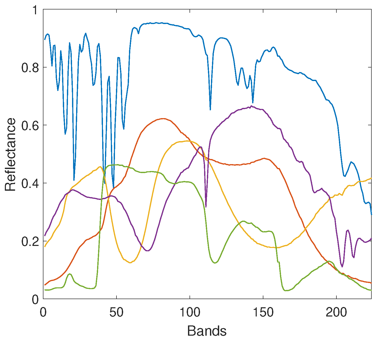
Experiments were firstly conducted on two sets of synthetic data cubes, namely DC1 and DC2 [21,22,34], that were generated by MLM [17] and PPNMM [16], respectively. For either set, there are three images, and each has a size of pixels. There are five endmembers for data generation, i.e., , that were randomly selected from the USGS library [35], each one being measured over 224 bands, as shown in Figure 1. The generated abundance maps corresponding to the five endmembers are illustrated in the first line of 5.
There are 25 regions of square in the image, each of the size pixels. Each square is homogeneous in terms of fractional abundances, namely the pixels in a same square have the same abundance vectors. The five squares of the first row are pure regions, each composed by only one endmember. For example, the abundance vectors for the square located at the first row and first column are . The five squares of the second row are mixed by two of the endmembers with the same proportions. Taking the square located at the second row and first column as an example, the corresponding abundance vectors are . Furthermore, the five squares in the last row of the image is a mixture of five endmembers with equal fractions, therefore they are identical. Apart from the 25 squares, the rest pixels in the image are all considered as background, which were generated using the following abundance vector . Generally, every synthetic image was generated using the aforementioned endmembers and abundance maps, according to different mixture models. The mixing models, as well as the associated parameters for generating DC1 and DC2, are detailed as follows:
- DC1:
- The pixels in DC1 images are generated by MLM in Equation (1). Specifically, the nonlinear probability parameter P is distributed as follows: the p values for the background pixels are set to zero by assuming that the backgrounds are linearly mixed. Concerning the remaining 25 regions in the square, each one is assigned by an identical p value, which is randomly chosen from a half-normal distribution with . The values of p larger than one are set to zero as in [17]. It is also noteworthy that, since the five squares in the last row are identical, the same p value is assigned to all of them.
- DC2:
- The synthetic pixels in DC2 images are generated based on the PPNMM [16], which is given bywhere the nonlinear parameter b is generated similarly as in DC1. For the assemblage of background pixels and the remaining 25 squares, each is assigned by the same b randomly drawn from a uniform distribution within the range , according to Altmann et al. [16].
Finally, to test the robustness of the proposed G-MLM against noise, the Gaussian noise of varying signal-to-noise ratio (SNR) is added, with dB, thus yielding three images for each set.
4.1.1. Experimental Setting
For all the comparing methods, the unmixing procedure was performed in a supervised manner, where the ground truth endmembers were utilized. Concerning the initialization of abundance matrix, the result of FCLS was applied in all methods. The parameters in state-of-the-art methods C-SUnSAL, GBM, PPNMM and MLM were basically set according to their original papers. Specifically, a supervised version of MLMp method was considered by simply fixing the endmembers in the algorithm, and the tolerance value was changed to from as in [18], for the sake of fair comparison. Regarding BNLSU, the maximum iteration number was set to 500, the tolerance value was set to , and the parameters were set as follows: the penalty parameter in ADMM was set as , and the regularization parameters in Equation (4) were set as for the sparsity constraint and for the smoothness of nonlinearity matrix, following the analysis in [20].
As for the proposed G-MLM algorithm, the maximum iteration number was set to 500, the tolerance value was set to , and the penalty parameter in ADMM was set as . Four regularization parameters needed to be tuned: , , and . To keep the comparison fair and also to simplify the process of parameters tuning, we fixed the parameter for sparsity regularization as , the same value as in BNLSU.
The threshold parameter in Equation (6) determines the affinity matrix computed from the input image, and should be chosen case by case. In essence, this parameter determines the underlying graph structure of the Laplacian regularizers on both abundance matrix and nonlinearity parameter vector, that is, only the pixels connected by nonzero elements in will mutually influence the parameter estimation. Following the spirit of the work in [36,37], we propose to estimate the parameter as a function of reconstruction error, by using an empirical formula
where the parameter was chosen as throughout the experiments, and is the abundance matrix estimated by FCLS [5]. In this way, the threshold parameter was chosen as 0.28, 0.17 and 0.13 for DC1 data with dB, respectively, and was chosen as 0.19, 0.08 and 0.05 for DC2 data with dB, respectively. Of particular note is that the dataset with lower SNR value generally prefers more important threshold value. It is reasonable, since severer noise affects the measure of the real similarity between spectra pairs more.
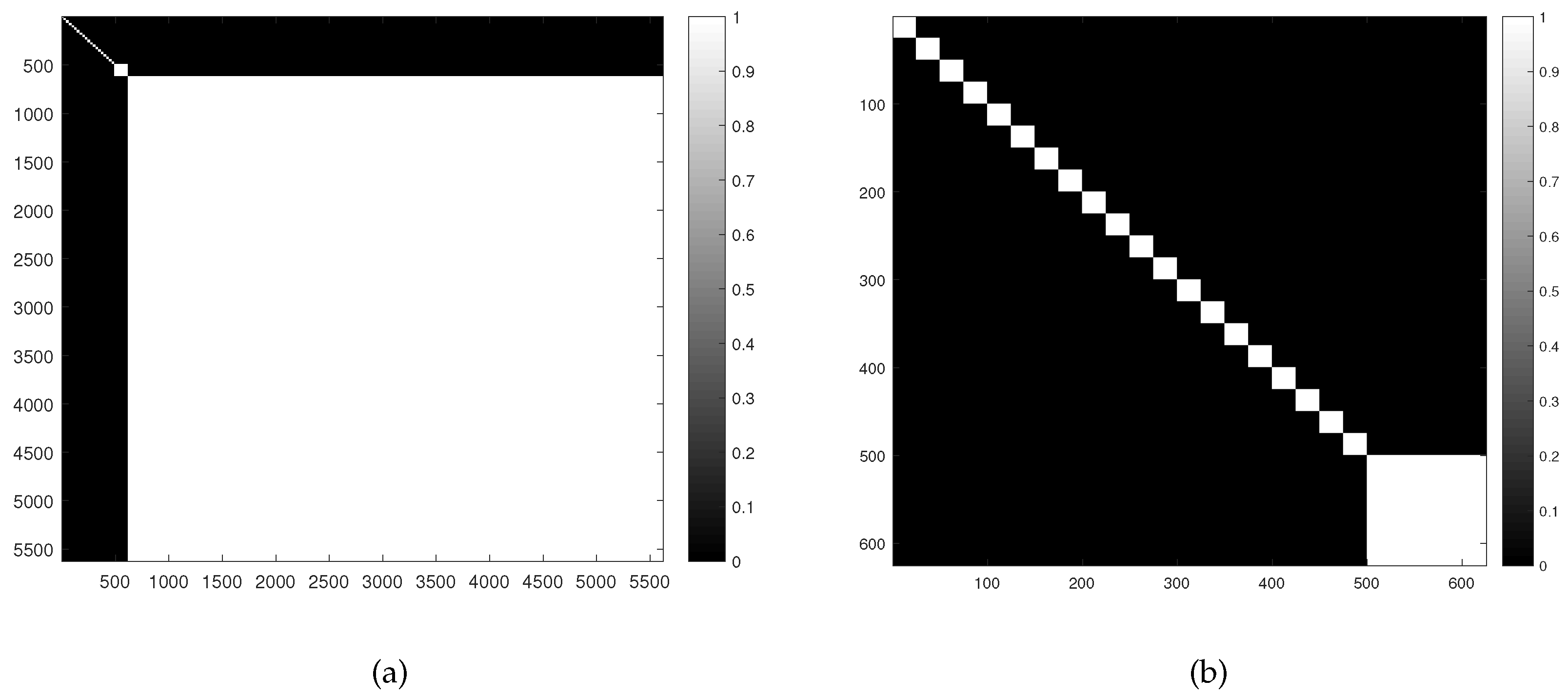
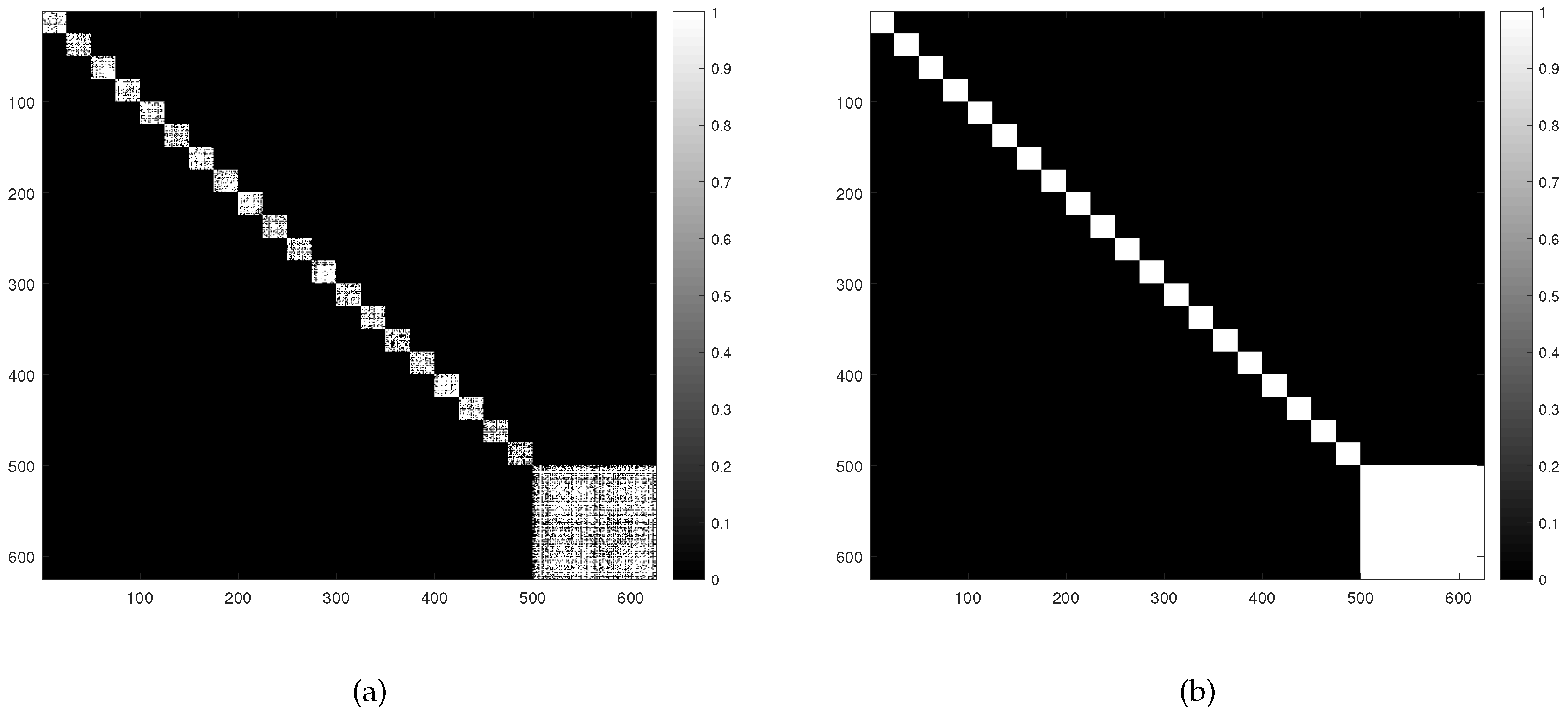
We verified the appropriateness of the parameter given by Equation (35), by taking DC1 data at dB as an example. For these data, the affinity matrix obtained by is shown in Figure 2, where a re-arranged matrix is shown for illustration purpose, according to Ammanouil et al. [24]. That is, the pixels of the five squares in the first row are placed first, then the pixels of the five squares in the second row appear, and so on, and the background pixels are placed last. We observe that there are 20 small, 1 medium and 1 big white blocks in . Each white block is a sub-matrix of whose elements are all close to 1, signifying the associated pixels are mutually similar. This is just consistent with the actual case of data generation. To be precise, the 20 small blocks correspond to the 20 different squares of pixels in the first four rows, each containing identical pixels; the one medium white block corresponds to an assemblage identical pixels from five squares in the last row; and the one big white block represents the sub-affinity-matrix for all the remaining identical background pixels. As a result, the graph structure of these data is well-revealed by obtained by . In Figure 3, we also compare the affinity matrices produced by and given by Equation (35), respectively. It is obvious that, with , the graph structure is better represented, with the resulting matrix being more consistent to the actual one. Based on above discussions, the effectiveness of Equation (35) in estimating is verified to some extent.
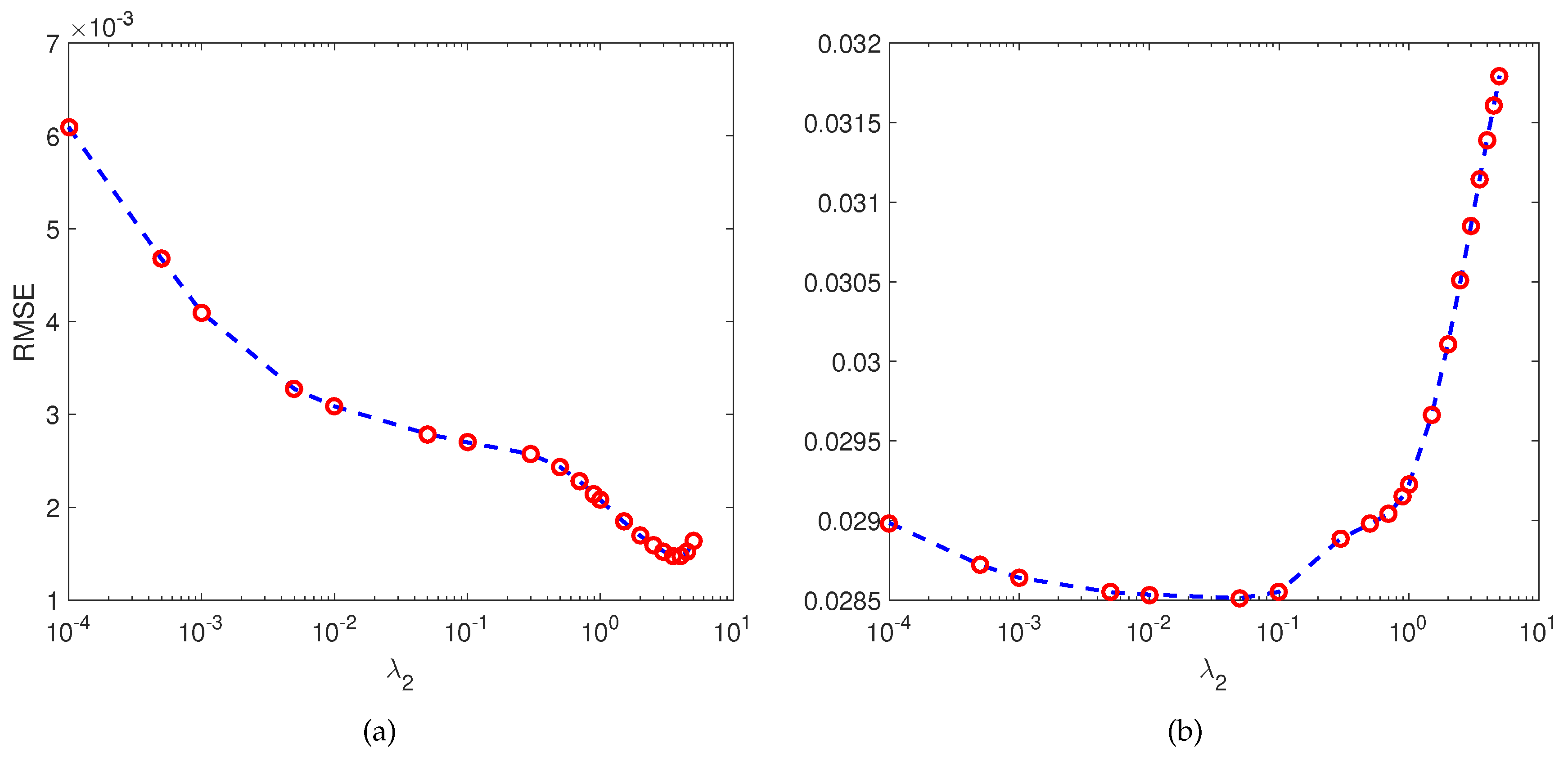
The remaining two regularization parameters to be tuned are and , which determine the importances of the graph-based abundance and nonlinearity parameter regularization terms, respectively. To further simplify the parameter tuning process, we applied in this experiment, considering that the abundance matrix has more dimensions than the nonlinear parameter . The parameter was then selected by applying the candidate value set , on the image with dB for each set. The influence of on unmixing performance in terms of RMSE is plotted in Figure 4a,b, where good results are obtained within the interval and for DC1 and DC2, respectively. Thus, we fixed for DC1, and for DC2.
4.1.2. Results Analysis
On images in DC1 and DC2, the unmixing performance was evaluated by the RMSE of abundance, as defined in Equation (32). The results obtained by applying all the comparing algorithms on DC1 and DC2 images at different noise levels are compared in Table 2 and Table 3, respectively. As observed in Table 2 for DC1, for all the three noise levels, the proposed G-MLM always outperforms its counterparts, by yielding the smallest RMSE value. This result is not surprising, as the proposed G-MLM takes advantage of the graph information hidden in the dataset, which is more consistent with the real situation. Moreover, as the value of SNR increases, the value of RMSE decreases prominently for every method. Namely, high noise level with low SNR deteriorates the performances of all the unmixing strategies. Generally, the MLM-based methods provide better unmixing results than the methods based on linear or bilinear models, on DC1.
In Table 3 for DC2, as the pixels were generated by PPNMM, it is not surprising to observe that the PPNMM unmixing method outperforms all the comparing methods. The proposed G-MLM is able to provide good unmixing results that are only second to those of PPNMM, on DC2 images with and . For the image with , it is the BNLSU method that yields the second best RMSE.
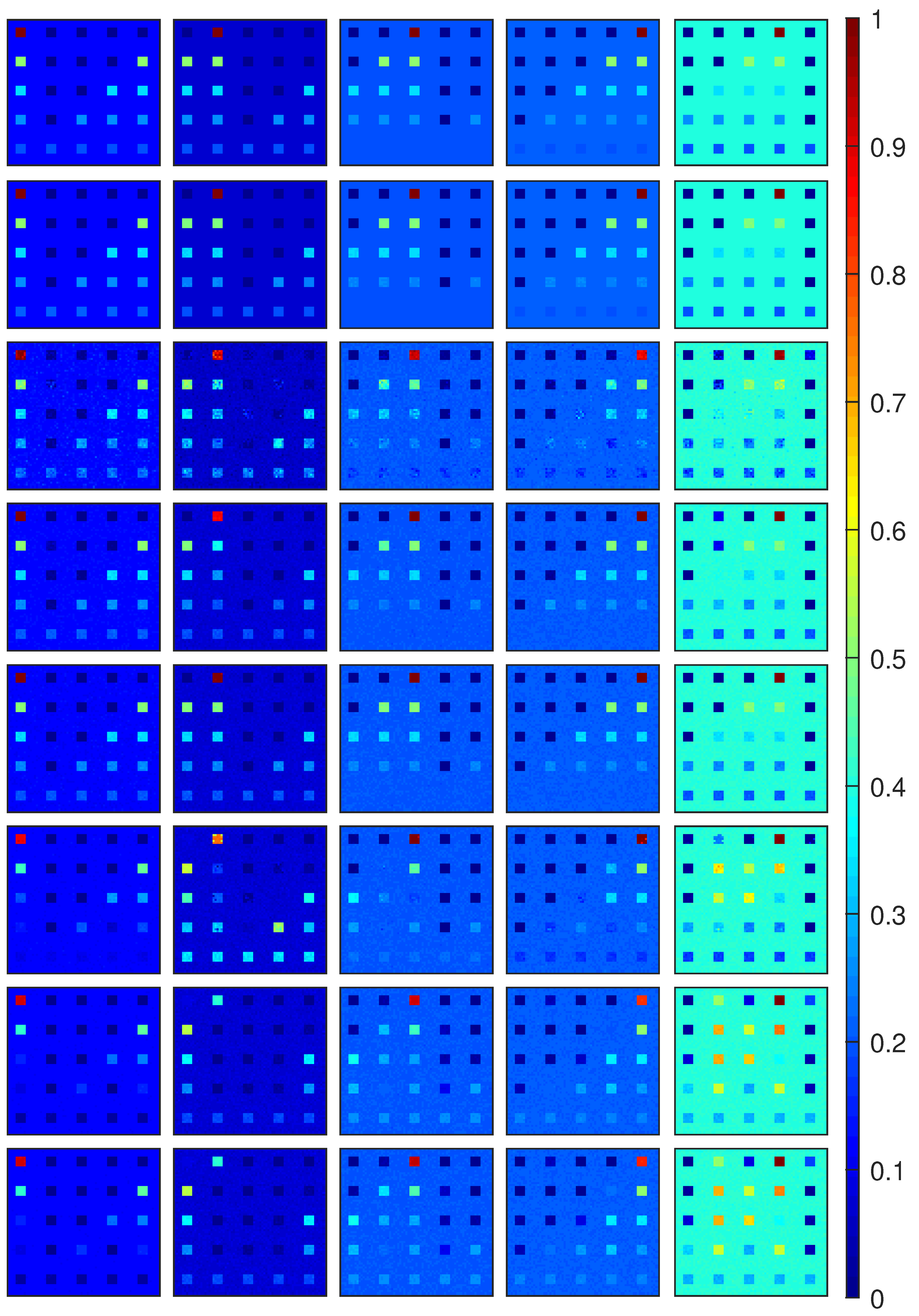
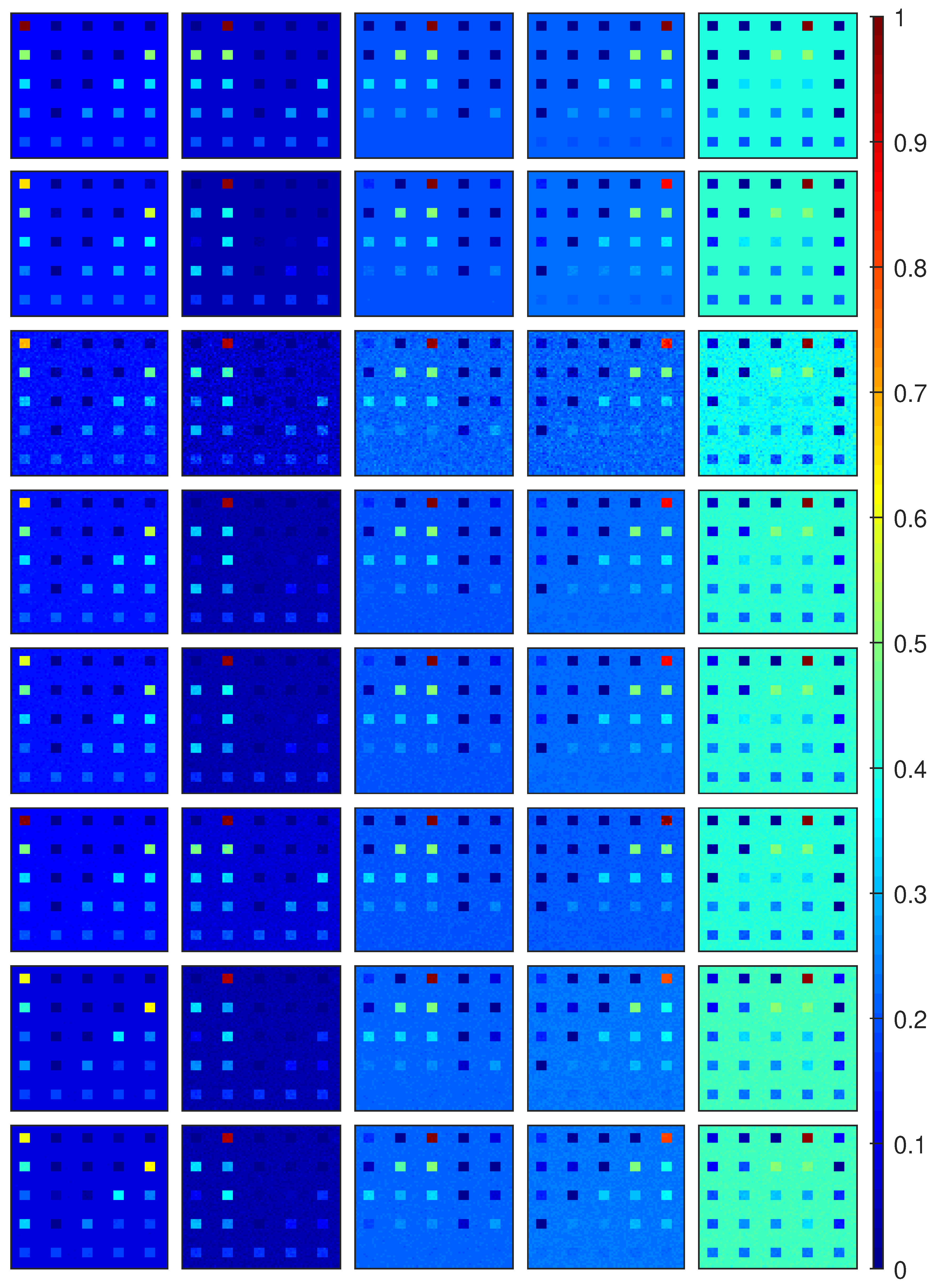
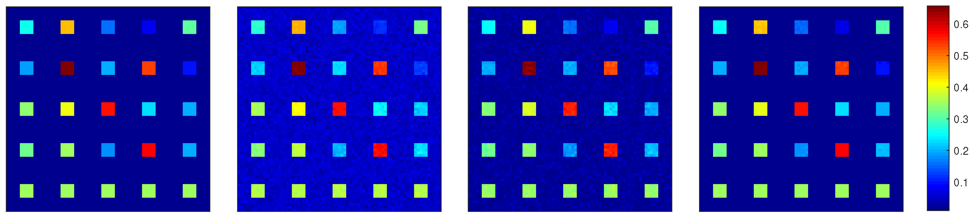
The estimated abundance maps by using different methods are shown in Figure 5 for DC1 image with SNR = 30, and in Figure 6 for DC2 image with SNR = 30. It is not difficult to find that the abundance maps obtained by the proposed G-MLM are the closest to the ground truth, when compared to all the other methods. For DC1 image with SNR = 30, the corresponding maps of P obtained by the MLM-based unmixing methods are shown in Figure 7, where the proposed G-MLM leads to the P map most consistent to the ground turth.
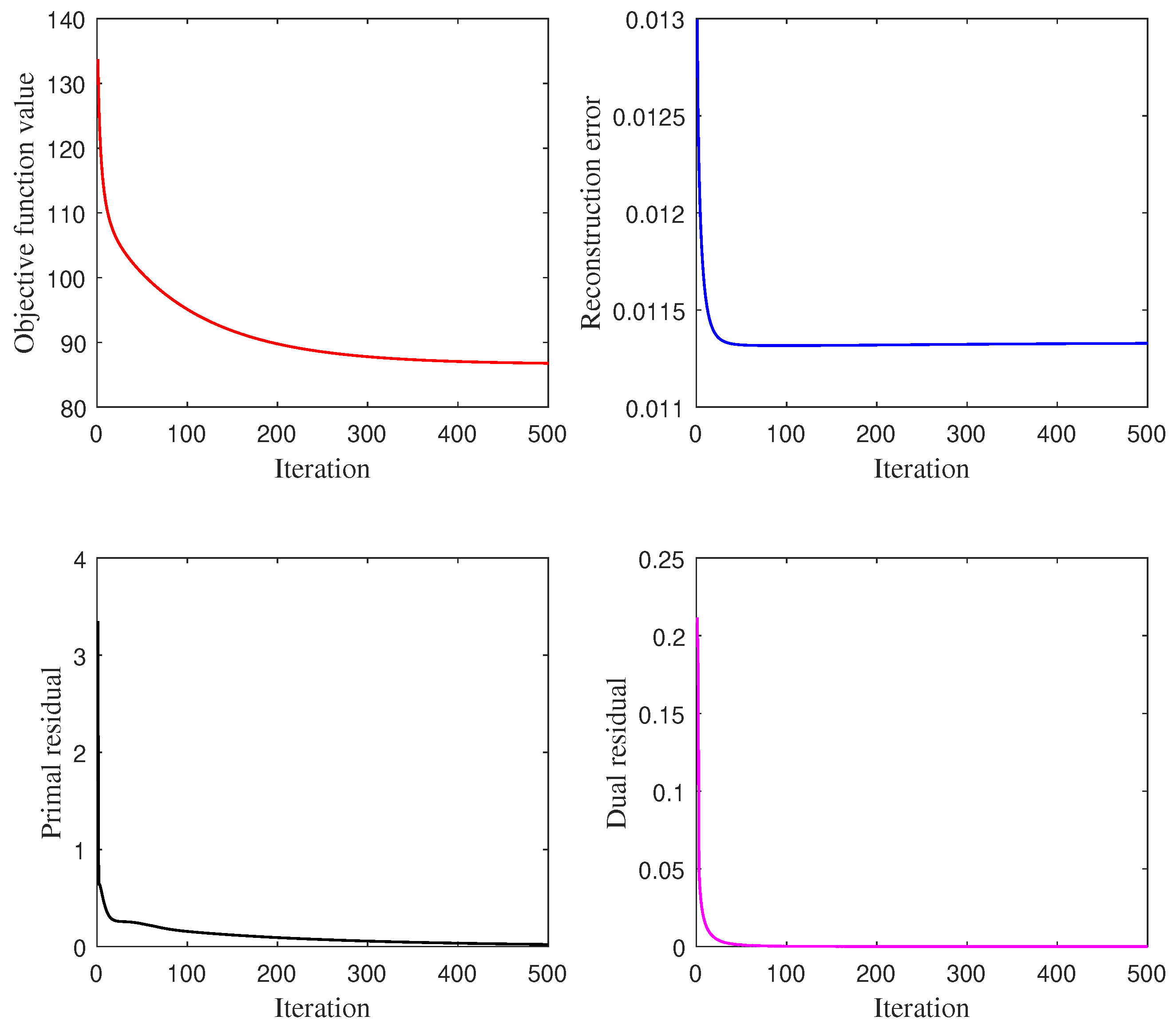
To study the convergence of the proposed ADMM algorithm for G-MLM, we traced the value of the objective function in Equation (9), the reconstruction error, the primal residual and the dual residual along with the number of iterations, as given in Figure 8. It is observed that all these values drop rapidly for the first 50 iterations, and then nearly decline to zeros at a slower rate. It demonstrates the good convergence of the proposed ADMM algorithm, according to [6,29].
Lastly, the executing time by different methods are compared in Table 4. The original G-MLM is shown to be time-consuming. To alleviate this issue, we examine and algorithms. The comparison of these three methods are reported in Table 5, where the number of clusters in is set as and the number of superpixels in is set as . As observed, the use of algorithm slightly reduces the computational time of G-MLM, almost without deteriorating the unmixing performance. The algorithm can greatly save the computational time, while providing acceptable RMSE that is still smaller than that of the comparing methods in Table 2. It is noteworthy that the overriding merit of is the practicality for addressing large-scale images, especially in the cases where both G-MLM and may not be applicable.
4.2. Experiments on Urban Dataset
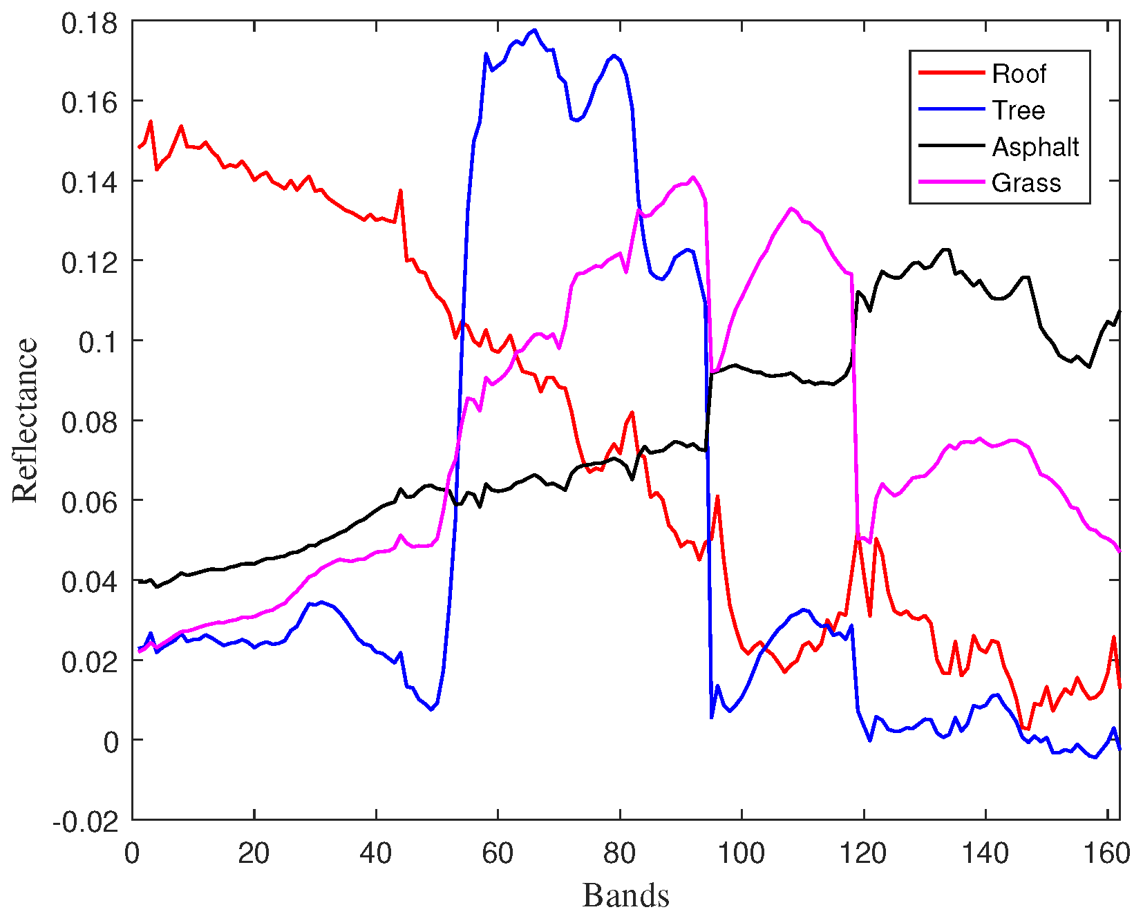
The Urban dataset is widely-investigated in hyperspectral unmixing research [9,38]. The original image has pixels with each pixel corresponding to an area of m area. It is measured by 210 wavelengths ranging from 400 nm to 2500 nm. After removing the noisy bands (1–4, 76, 87, 101–111, 136–153, and 198–210) that are contaminated by water vapor density and atmosphere, the remaining 162 bands of high SNR were considered. This field is known to be mainly composed by four materials: roof, tree, asphalt and grass. In our experiment, the four endmembers were first extracted by the VCA algorithm, as shown in Figure 9.
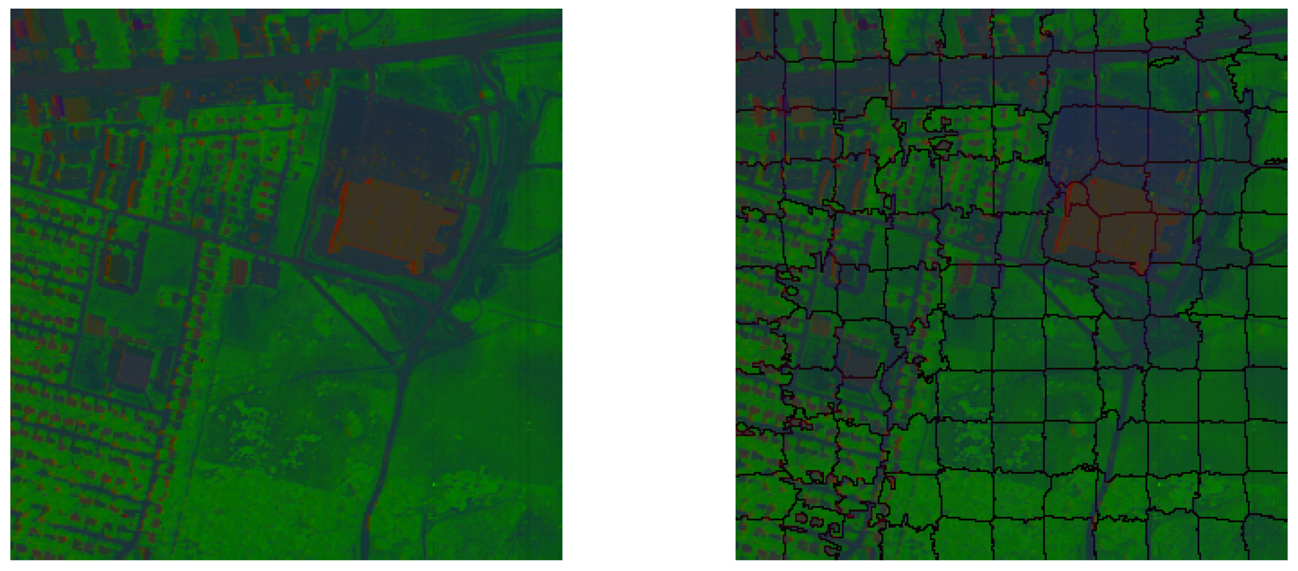
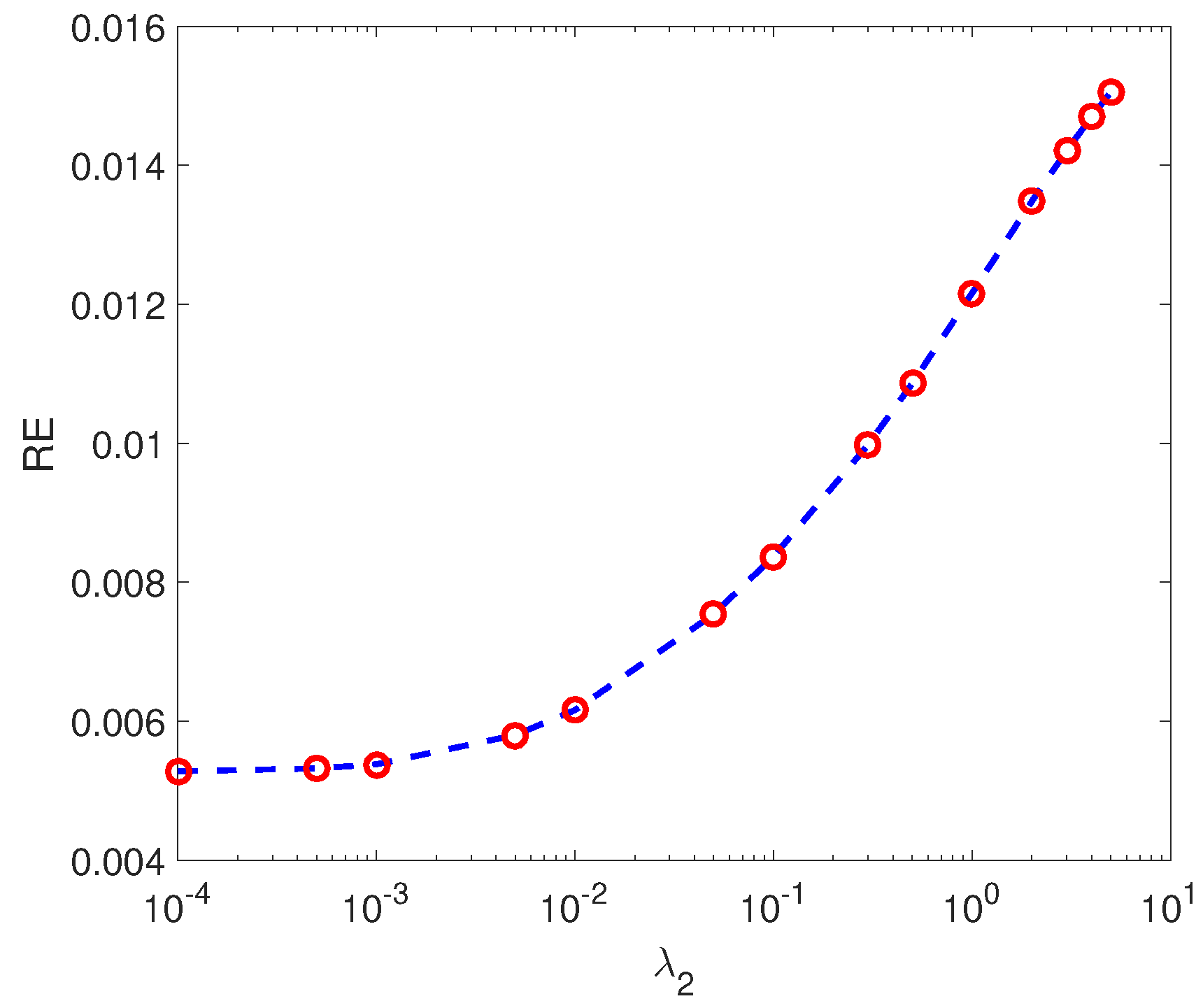
Because the Urban image is of large scale, neither G-MLM nor can be directly applied on our computer. Therefore, the scheme was adopted. We speciied the selection of parameters in for Urban image. The original image was firstly divided into superpixels, as shown in Figure 10. The value of in Equation (6) was estimated to be 0.02, according to Equation (35). As done for synthetic images, the sparsity regularization parameter was set as , and the relationship with was maintained. For Urban image, the value of was selected from the set . For illustration purposes, we plot the changes of RE along with in Figure 11. It is observed that the RE value is relatively small and stable for small values of , and starts to increase when exceeds 0.001. Therefore, we chose for Urban image.
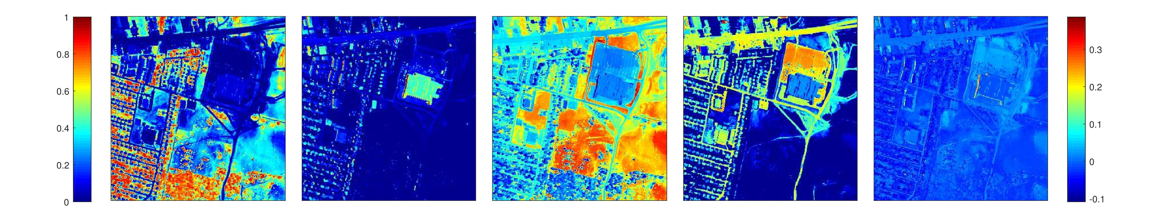
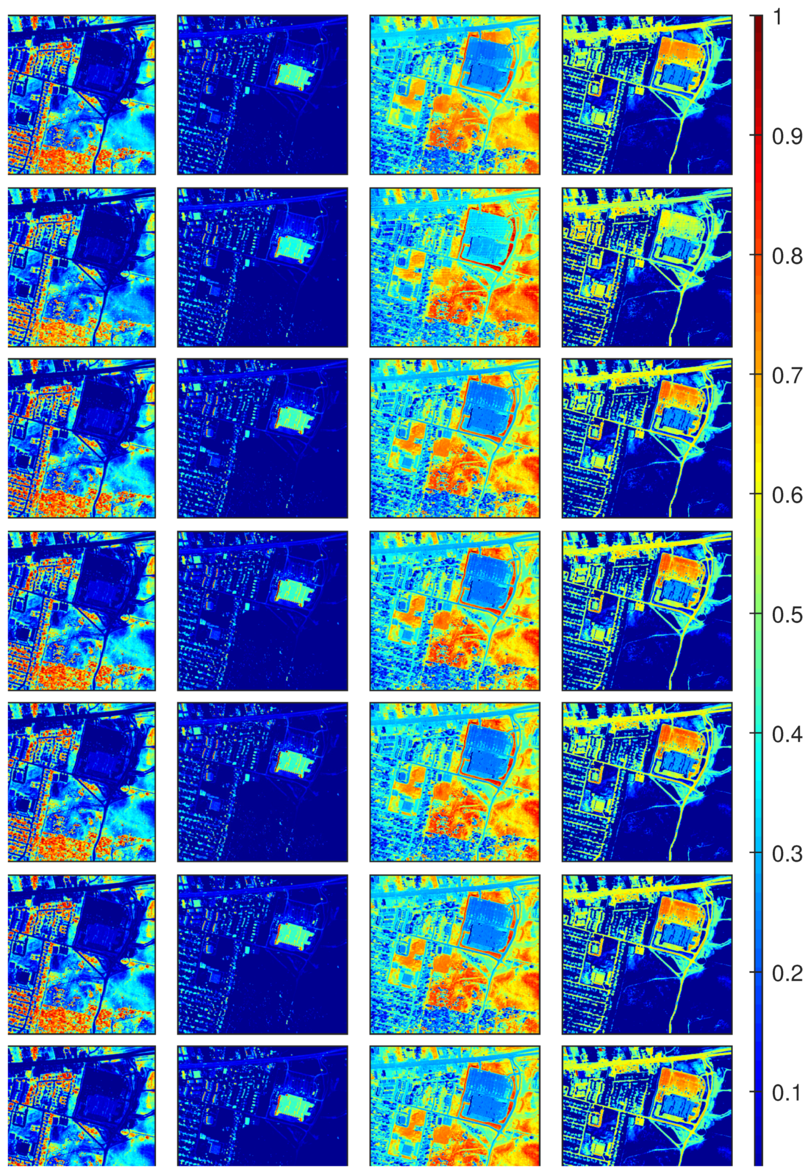
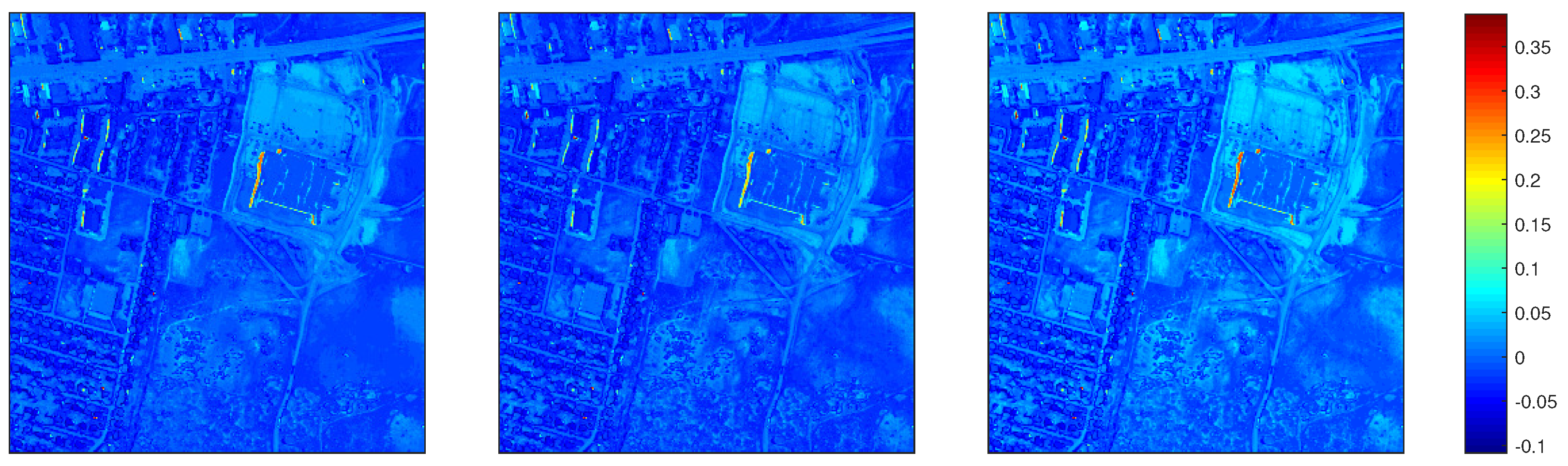
The executing time using all the comparing methods is given in Table 6. A comparison of RE is also reported in the same table, where BNLSU provides a value much smaller than other unmixing approaches. It is reasonable, as this method defines the nonlinearity parameter in each band for a given pixel, thus yielding a model with many more parameters to fit the reconstruction error, compared to other methods. However, it should be noticed that RE is only adopted as a reference of the unmixing performance. It measures the averaged fitting level of a mixture model, e.g., LMM, GBM or MLM, to the observed spectra, but cannot truly reflect the unmixing quality in terms of abundance, especially for real hyperspectral images where the mechanism of mixture is complicated and unclear [10]. The abundance maps obtained by all comparing algorithms are shown in Figure 12. The abundance maps by different algorithms visually show little differences. The estimated maps of P obtained with , MLM and MLMp are shown in Figure 13. All three maps correspond well with the areas in the image where nonlinear effects are expected to be significant, e.g., the intersection area between roof and tree, and between grass and asphalt. As the graph structure of data is considered in the proposed , the corresponding abundance maps and P map exhibit more spatial consistency and and smoothness compared with other algorithms.
5. Conclusions
This paper proposes a graph regularized hyperspectral unmixing method based on the multilinear mixing model. By taking advantage of the graph structure embedded in the data, Laplacian graph ragularizers are introduced to regularize both the abundance matrix and the nonlinear probability parameters. The sparse constraint is also enforced on the abundance matrix. The resulting optimization problem is solved by using ADMM algorithm, and the superpixel construction scheme is applied to reduce the complexity. Comparative studies on two series of synthetic data and a real hyperspectral image verified the advantage of the proposed algorithm in terms of unmixing results. Future works include jointly exploiting the graph and spatial structures to further augment the G-MLM model, in order to accurately characterize abundances and nonlinear probability parameters. Extending the nonlinear parameters in G-MLM model to a band-wise form is also worth our investigation.
Author Contributions
F.Z. and M.L. conceived the idea and developed the methodology; M.L. prepared the first draft; and A.J.X.G. and J.C. contributed to the synthetic data preparation and experimental analysis.
Funding
The work was supported by the National Natural Science Foundation of China under Grant 61701337 and Grant 61671382, and the Natural Science Foundation of Tianjin City under Grant 18JCQNJC01600.
Acknowledgments
The authors would like to thank Q. Wei for sharing the MLMp code, and B. Yang for sharing the BNLSU code.
Conflicts of Interest
The authors declare no conflict of interest.
References
- Bioucas-Dias, J.M.; Plaza, A.; Dobigeon, N.; Parente, M.; Du, Q.; Gader, P.; Chanussot, J. Hyperspectral Unmixing Overview: Geometrical, Statistical, and Sparse Regression-Based Approaches. IEEE J. Sel. Top. Appl. Earth Obs. Remote Sens. 2012, 5, 354–379. [Google Scholar] [CrossRef] [Green Version]
- Dobigeon, N.; Tourneret, J.; Richard, C.; Bermudez, J.C.M.; McLaughlin, S.; Hero, A.O. Nonlinear Unmixing of Hyperspectral Images: Models and Algorithms. IEEE Signal Process. Mag. 2014, 31, 82–94. [Google Scholar] [CrossRef]
- Keshava, N.; Mustard, J.F. Spectral unmixing. IEEE Signal Process. Mag. 2002, 19, 44–57. [Google Scholar] [CrossRef]
- Adams, J.; Smith, M.O. Spectral Mixture Modeling: A new analysis of rock and soil types at the Viking Lander 1 Site. J. Geophys. Res. 1986, 91, 8098–8112. [Google Scholar] [CrossRef]
- Heinz, D.C.; Chang, C.I. Fully Constrained Least Squares Linear Spectral Mixture Analysis Method for Material Quantification in Hyperspectral Imagery. IEEE Trans. Geosci. Remote Sens. 2001, 39, 529–545. [Google Scholar] [CrossRef]
- Bioucas-Dias, J.M.; Figueiredo, M.A.T. Alternating direction algorithms for constrained sparse regression: Application to hyperspectral unmixing. In Proceedings of the 2010 2nd Workshop on Hyperspectral Image and Signal Processing: Evolution in Remote Sensing, Reykjavik, Iceland, 14–16 June 2010; pp. 1–4. [Google Scholar] [CrossRef]
- Heylen, R.; Parente, M.; Gader, P. A Review of Nonlinear Hyperspectral Unmixing Methods. IEEE J. Sel. Top. Appl. Earth Obs. Remote Sens. 2014, 7, 1844–1868. [Google Scholar] [CrossRef]
- Hapke, B. Bidirectional reflectance spectroscopy: 1. Theory. J. Geophys. Res. Solid Earth 1981, 86, 3039–3054. [Google Scholar] [CrossRef]
- Zhu, F.; Honeine, P. Bi-Objective Nonnegative Matrix Factorization: Linear Versus Kernel-Based Models. IEEE Trans. Geosci. Remote Sens. 2016, 54, 4012–4022. [Google Scholar] [CrossRef]
- Chen, J.; Richard, C.; Honeine, P. Nonlinear unmixing of hyperspectral data based on a linear-mixture/nonlinear-fluctuation model. IEEE Trans. Signal Process. 2013, 61, 480–492. [Google Scholar] [CrossRef]
- Huete, A.R.; Jackson, R.D.; Post, D.F. Spectral response of a plant canopy with different soil backgrounds. Remote Sens. Environ. 1985, 17, 37–53. [Google Scholar] [CrossRef]
- Nascimento, J.M.P.; Dias, J.M.B. Nonlinear mixture model for hyperspectral unmixing. In Proceedings of the Image and Signal Processing for Remote Sensing XV, Berlin, Germany, 31 August–3 September 2009; Volume 7477. [Google Scholar] [CrossRef]
- Fan, W.; Hu, B.; Miller, J.; Li, M. Comparative study between a new nonlinear model and common linear model for analysing laboratory simulated-forest hyperspectral data. Int. J. Remote Sens. 2009, 30, 2951–2962. [Google Scholar] [CrossRef]
- Halimi, A.; Altmann, Y.; Dobigeon, N.; Tourneret, J. Nonlinear unmixing of hyperspectral images using a generalized bilinear model. In Proceedings of the 2011 IEEE Statistical Signal Processing Workshop (SSP), Nice, France, 28–30 June 2011; pp. 413–416. [Google Scholar] [CrossRef]
- Yokoya, N.; Chanussot, J.; Iwasaki, A. Nonlinear Unmixing of Hyperspectral Data Using Semi-Nonnegative Matrix Factorization. IEEE Trans. Geosci. Remote Sens. 2014, 52, 1430–1437. [Google Scholar] [CrossRef]
- Altmann, Y.; Halimi, A.; Dobigeon, N.; Tourneret, J. Supervised Nonlinear Spectral Unmixing Using a Postnonlinear Mixing Model for Hyperspectral Imagery. IEEE Trans. Image Process. 2012, 21, 3017–3025. [Google Scholar] [CrossRef] [Green Version]
- Heylen, R.; Scheunders, P. A Multilinear Mixing Model for Nonlinear Spectral Unmixing. IEEE Trans. Geosci. Remote Sens. 2016, 54, 240–251. [Google Scholar] [CrossRef]
- Wei, Q.; Chen, M.; Tourneret, J.; Godsill, S. Unsupervised Nonlinear Spectral Unmixing Based on a Multilinear Mixing Model. IEEE Trans. Geosci. Remote Sens. 2017, 55, 4534–4544. [Google Scholar] [CrossRef] [Green Version]
- Nascimento, J.M.P.; Dias, J.M.B. Vertex component analysis: A fast algorithm to unmix hyperspectral data. IEEE Trans. Geosci. Remote Sens. 2005, 43, 898–910. [Google Scholar] [CrossRef]
- Yang, B.; Wang, B. Band-Wise Nonlinear Unmixing for Hyperspectral Imagery Using an Extended Multilinear Mixing Model. IEEE Trans. Geosci. Remote Sens. 2018, 56, 6747–6762. [Google Scholar] [CrossRef]
- Chen, J.; Richard, C.; Honeine, P. Nonlinear Estimation of Material Abundances in Hyperspectral Images with ℓ1-Norm Spatial Regularization. IEEE Trans. Geosci. Remote Sens. 2014, 52, 2654–2665. [Google Scholar] [CrossRef]
- Iordache, M.; Bioucas-Dias, J.M.; Plaza, A. Total Variation Spatial Regularization for Sparse Hyperspectral Unmixing. IEEE Trans. Geosci. Remote Sens. 2012, 50, 4484–4502. [Google Scholar] [CrossRef] [Green Version]
- Lu, X.; Wu, H.; Yuan, Y.; Yan, P.; Li, X. Manifold Regularized Sparse NMF for Hyperspectral Unmixing. IEEE Trans. Geosci. Remote Sens. 2013, 51, 2815–2826. [Google Scholar] [CrossRef]
- Ammanouil, R.; Ferrari, A.; Richard, C. A graph Laplacian regularization for hyperspectral data unmixing. In Proceedings of the 2015 IEEE International Conference on Acoustics, Speech and Signal Processing (ICASSP), Brisbane, Australia, 19–24 April 2015; pp. 1637–1641. [Google Scholar] [CrossRef]
- Shi, C.; Wang, L. Incorporating spatial information in spectral unmixing: A review. Remote Sens. Environ. 2014, 149, 70–87. [Google Scholar] [CrossRef]
- Qian, Y.; Jia, S.; Zhou, J.; Robles-Kelly, A. Hyperspectral Unmixing via L1/2 Sparsity-Constrained Nonnegative Matrix Factorization. IEEE Trans. Geosci. Remote Sens. 2011, 49, 4282–4297. [Google Scholar] [CrossRef]
- Zhu, F.; Honeine, P.; Kallas, M. Kernel nonnegative matrix factorization without the pre-image problem. In Proceedings of the IEEE International Workshop on Machine Learning for Signal Processing, Reims, France, 21–24 September 2014. [Google Scholar]
- Li, Z.; Chen, J.; Rahardja, S. Superpixel construction for hyperspectral unmixing. In Proceedings of the 2018 26th European Signal Processing Conference (EUSIPCO), Rome, Italy, 3–7 September 2018; pp. 647–651. [Google Scholar] [CrossRef]
- Boyd, S.; Parikh, N.; Chu, E.; Peleato, B.; Eckstein, J. Distributed Optimization and Statistical Learning via the Alternating Direction Method of Multipliers. Found. Trends Mach. Learn. 2011, 3, 1–122. [Google Scholar]
- Iordache, M.; Bioucas-Dias, J.M.; Plaza, A. Sparse Unmixing of Hyperspectral Data. IEEE Trans. Geosci. Remote Sens. 2011, 49, 2014–2039. [Google Scholar] [CrossRef] [Green Version]
- Guo, Z.; Wittman, T.; Osher, S. L1 unmixing and its application to hyperspectral image enhancement. In Proceedings of the Algorithms and Technologies for Multispectral, Hyperspectral, and Ultraspectral Imagery XV, 73341M, Orlando, FL, USA, 13–17 April 2009; Volume 7334. [Google Scholar] [CrossRef]
- Winter, M. N-FINDR: An algorithm for fast autonomous spectral end-member determination in hyperspectral data: An algorithm for fast autonomous spectral end-member determination in hyperspectral data. In Proceedings of the Imaging Spectrometry V, Denver, CO, USA, 18–23 July 1999; Volume 3753, pp. 266–275. [Google Scholar]
- Ng, A.; Jordan, M.; Weiss, Y. On Spectral Clustering: Analysis and an Algorithm. In Proceedings of the 14th International Conference on Neural Information Processing Systems: Natural and Synthetic (NIPS’01), Vancouver, BC, Canada, 3–8 December 2001; MIT Press: Cambridge, MA, USA, 2001; pp. 849–856. [Google Scholar]
- Wang, Y.; Pan, C.; Xiang, S.; Zhu, F. Robust Hyperspectral Unmixing with Correntropy-Based Metric. IEEE Trans. Image Process. 2015, 24, 4027–4040. [Google Scholar] [CrossRef]
- Bioucas-Dias, J.M.; Nascimento, J.M.P. Hyperspectral Subspace Identification. IEEE Trans. Geosci. Remote Sens. 2008, 46, 2435–2445. [Google Scholar] [CrossRef] [Green Version]
- He, R.; Zheng, W.S.; Hu, B.G. Maximum Correntropy Criterion for Robust Face Recognition. IEEE Trans. Pattern Anal. Mach. Intell. 2011, 33, 1561–1576. [Google Scholar]
- Zhu, F.; Halimi, A.; Honeine, P.; Chen, B.; Zheng, N. Correntropy Maximization via ADMM: Application to Robust Hyperspectral Unmixing. IEEE Trans. Geosci. Remote Sens. 2017, 55, 4944–4955. [Google Scholar] [CrossRef] [Green Version]
- Zhu, F.; Wang, Y.; Fan, B.; Xiang, S.; Meng, G.; Pan, C. Spectral Unmixing via Data-Guided Sparsity. IEEE Trans. Image Process. 2014, 23, 5412–5427. [Google Scholar] [CrossRef]
Figure 1.
Five endmembers selected from the USGS library for generating DC1 and DC2 images.

Figure 2.
Visualization of affinity matrix with for the DC1 image with SNR = 30 dB: (a) the full ; and (b) the sub-matrix of by removing all the background pixels.
Figure 2.
Visualization of affinity matrix with for the DC1 image with SNR = 30 dB: (a) the full ; and (b) the sub-matrix of by removing all the background pixels.

Figure 3.
Visualizations of affinity matrix of by removing all the background pixels, for the DC1 image with SNR = 25 dB: (a) ; and (b) given by Equation (35).
Figure 3.
Visualizations of affinity matrix of by removing all the background pixels, for the DC1 image with SNR = 25 dB: (a) ; and (b) given by Equation (35).

Figure 4.
The changes of RMSE along with different values of : (a) DC1 image with SNR = 30 dB; and (b) DC2 image with SNR = 30 dB.
Figure 4.
The changes of RMSE along with different values of : (a) DC1 image with SNR = 30 dB; and (b) DC2 image with SNR = 30 dB.

Figure 5.
Estimated abundance maps on DC1 image with SNR = 30, obtained by using different comparing methods. From top to bottom: Ground truth, G-MLM, BNLSU, MLMp, MLM, PPNMM, GBM and FCLS. From left to right: endmember .
Figure 5.
Estimated abundance maps on DC1 image with SNR = 30, obtained by using different comparing methods. From top to bottom: Ground truth, G-MLM, BNLSU, MLMp, MLM, PPNMM, GBM and FCLS. From left to right: endmember .

Figure 6.
Estimated abundance maps on DC2 image with SNR = 30, obtained by using different comparing methods. From top to bottom: Ground truth, G-MLM, BNLSU, MLMp, MLM, PPNMM, GBM and FCLS. From left to right: endmember .
Figure 6.
Estimated abundance maps on DC2 image with SNR = 30, obtained by using different comparing methods. From top to bottom: Ground truth, G-MLM, BNLSU, MLMp, MLM, PPNMM, GBM and FCLS. From left to right: endmember .

Figure 7.
Estimated map of P by different MLM-based unmixing methods. From left to right: Groundtruth, MLM, MLMp, and G-MLM, on DC1 image with SNR = 30 dB.
Figure 7.
Estimated map of P by different MLM-based unmixing methods. From left to right: Groundtruth, MLM, MLMp, and G-MLM, on DC1 image with SNR = 30 dB.

Figure 8.
Illustration of the convergence of G-MLM, by the objective function value, reconstruction error, primal residual and dual residual over 500 iterations.
Figure 8.
Illustration of the convergence of G-MLM, by the objective function value, reconstruction error, primal residual and dual residual over 500 iterations.

Figure 9.
Four endmembers extracted by VCA, on Urban data.

Figure 10.
(Left) False color image of Urban data. (Right) Constructed superpixels with m = 120.

Figure 11.
The changes of RE obtained by along with different values of , on Urban image.

Figure 12.
Estimated abundance maps for Urban image. From left to right for different endmembers: tree, roof, grass and asphalt. From top to bottom for different methods: , BNLSU, MLMp, MLM, PPNMM, GBM, and FCLS.
Figure 12.
Estimated abundance maps for Urban image. From left to right for different endmembers: tree, roof, grass and asphalt. From top to bottom for different methods: , BNLSU, MLMp, MLM, PPNMM, GBM, and FCLS.

Figure 13.
Estimated map of P obtained by , MLMp, and MLM, on Urban dataset.


Table 1.
The complexity of the proposed G-MLM for updating each variable per iteration.
| Variable to Update | S | G | P | H | ||
|---|---|---|---|---|---|---|
| Complexity per Iteration |
Table 2.
The averaged RMSE values over five runs using all the comparing methods, on three DC1 datasets.
Table 2.
The averaged RMSE values over five runs using all the comparing methods, on three DC1 datasets.
| Methods | SNR 25 dB | SNR 30 dB | SNR 35 dB |
|---|---|---|---|
| G-MLM | 0.0049 () | 0.0015 () | 0.0006 () |
| BNLSU | 0.0479 | 0.0206 | 0.0113 |
| MLMp | 0.0194 | 0.0107 | 0.0061 |
| MLM | 0.0114 | 0.0065 | 0.0036 |
| PPNMM | 0.0375 | 0.0365 | 0.0360 |
| GBM | 0.0516 | 0.0509 | 0.0506 |
| FCLS | 0.0507 | 0.0499 | 0.0497 |
Table 3.
The averaged RMSE values over five runs by all the comparing methods, on three DC2 datasets.
Table 3.
The averaged RMSE values over five runs by all the comparing methods, on three DC2 datasets.
| Methods | SNR 25 dB | SNR 30 dB | SNR 35 dB |
|---|---|---|---|
| G-MLM | 0.0302 () | 0.0285 () | 0.0282 () |
| BNLSU | 0.0504 | 0.0306 | 0.0187 |
| MLMp | 0.0321 | 0.0297 | 0.0290 |
| MLM | 0.0311 | 0.0297 | 0.0292 |
| PPNMM | 0.0128 | 0.0075 | 0.0045 |
| GBM | 0.0389 | 0.0381 | 0.0378 |
| FCLS | 0.0388 | 0.0380 | 0.0377 |
Table 4.
Computational time measured by different algorithms on DC1 with SNR = 30 dB.
| Methods | Time [s] |
|---|---|
| G-MLM | 445.18 |
| BNLSU | 574.31 |
| MLMp | 69.43 |
| MLM | 118.88 |
| PPNMM | 235.50 |
| GBM | 34.25 |
| FCLS | 1.93 |
Table 5.
Comparison of RMSE and computational time of G-MLM, and on DC1 with SNR = 30 dB. The preprocessing time for and is omitted in the table.
Table 5.
Comparison of RMSE and computational time of G-MLM, and on DC1 with SNR = 30 dB. The preprocessing time for and is omitted in the table.
| Methods | RMSE | Time [s] |
|---|---|---|
| G-MLM | 0.0015 | 445.18 |
| G-MLMsub | 0.0015 | 402.29 |
| G-MLMsuper | 0.0027 | 152.42 |
Table 6.
Comparison of RE and computational time of , BNLSU, MLMp, MLM, PPNMM, GBM, and FCLS on Urabn image.
Table 6.
Comparison of RE and computational time of , BNLSU, MLMp, MLM, PPNMM, GBM, and FCLS on Urabn image.
| Methods | RE | Time [s] |
|---|---|---|
| 0.0053 | 1904.89 | |
| BNLSU | 0.0019 | 5443.02 |
| MLMp | 0.0053 | 26.77 |
| MLM | 0.0053 | 1075.40 |
| PPNMM | 0.0052 | 591.42 |
| GBM | 0.0056 | 72.37 |
| FCLS | 0.0056 | 19.09 |
© 2019 by the authors. Licensee MDPI, Basel, Switzerland. This article is an open access article distributed under the terms and conditions of the Creative Commons Attribution (CC BY) license (http://creativecommons.org/licenses/by/4.0/).
Share and Cite
MDPI and ACS Style
Li, M.; Zhu, F.; Guo, A.J.X.; Chen, J. A Graph Regularized Multilinear Mixing Model for Nonlinear Hyperspectral Unmixing. Remote Sens. 2019, 11, 2188. https://doi.org/10.3390/rs11192188
AMA Style
Li M, Zhu F, Guo AJX, Chen J. A Graph Regularized Multilinear Mixing Model for Nonlinear Hyperspectral Unmixing. Remote Sensing. 2019; 11(19):2188. https://doi.org/10.3390/rs11192188
Chicago/Turabian StyleLi, Minglei, Fei Zhu, Alan J. X. Guo, and Jie Chen. 2019. "A Graph Regularized Multilinear Mixing Model for Nonlinear Hyperspectral Unmixing" Remote Sensing 11, no. 19: 2188. https://doi.org/10.3390/rs11192188
Note that from the first issue of 2016, this journal uses article numbers instead of page numbers. See further details here.